Using Near-Surface Ground Temperature Data to Derive Snow Insulation and Melt Indices for Mountain Permafrost Applications

Using Near-Surface Ground Temperature Data to Derive Snow Insulation and Melt Indices for Mountain Permafrost Applications

Benno Staub* and Reynald Delaloye

University of Fribourg, Department of Geosciences, Geography, Fribourg, Switzerland

ABSTRACT

The timing and duration of snow cover in areas of mountain permafrost affect the ground thermal regime by ther- mally insulating the ground from the atmosphere and modifying the radiation balance at the surface. Snow depth re- cords, however, are sparse in high-mountain terrains. Here, we present data processing techniques to approximate the thermal insulation effect of snow cover. We propose some simple ‘ snow thermal insulation indices ’ using daily and weekly variations in ground surface temperatures (GSTs), as well as a ‘ snow melt index ’ that approximates the snow melt rate using a degree-day approach with air temperature during the zero curtain period. The indices consider point- speci fi c characteristics and allow the reconstruction of past snow thermal conditions and snow melt rates using long GST time series. The application of these indices to GST monitoring data from the Swiss Alps revealed large spatial and temporal variability in the start and duration of the high-insulation period by snow and in the snow melt rate.

KEY WORDS: mountain permafrost; ground surface temperature; thermal insulation; snow onset; snow water equivalent; snow melt rate

INTRODUCTION

Mountain permafrost environments higher than ~ 2500 m asl in the Swiss Alps (Noetzli and Gruber, 2005) are characterised by rough topography, highly variable micro- topoclimates and long-lasting seasonal snow cover. Snow accumulation, redistribution and melt strongly in fl uence the energy balance at the ground surface and thus the ground thermal regime (e.g. Goodrich, 1982; Hoelzle et al., 2001; Stocker-Mittaz et al., 2002). Accumulation of an insulating snow cover in autumn plays a key role on in- terannual ground temperature variations, because of its long-lasting effect throughout winter (Delaloye, 2004;

Marmy et al., 2013). The total quantity of snow melt and the melting rate per day are signi fi cant in the analysis of thawing processes in the active layer and the quanti fi cation of the in fl uence of meltwater in fi ltration on rock glacier ki- nematics. The development of the snow cover is regionally dependent on precipitation patterns and locally in fl uenced by wind, avalanches and radiation, factors that make its de- velopment highly variable in space and time (Gisnås et al., 2014; Laternser and Schneebeli, 2003). But snow data are

measured only at a few points. However, as ground surface temperatures (GSTs) are in fl uenced by the local snow characteristics, GST data recorded with common miniature temperature loggers (Hoelzle et al., 1999) can be used to ex- tract snow information directly at the points of interest for mountain permafrost research.

This paper uses GST time series to estimate the thermal in- sulation effect of the snow, from which periods of high insula- tion and snow melt can be delineated. It also approximates the snow melt rate (SMR) during zero curtain periods using a degree-day approach with air temperature (AirT). The applica- bility of these methods is demonstrated with selected GST monitoring time series from the Swiss Alps.

BACKGROUND

Relevance of the Seasonal Snow Cover for the Ground Thermal Regime

The thermal conductivity of snow ranges from 0.1 (fresh snow with a large fraction of air) to 0.5 (old snow with higher density) Wm

K

and is fi ve to 20 times lower than that of mineral soils (Zhang, 2005). Therefore, snow can thermally decouple the ground from the atmosphere with in- creasing snow depth. According to the literature, snow

*Correspondence to: B. Staub, University of Fribourg, Department of Geosciences, Geography, Chemin du Musée 4, CH-1700 Fribourg, Switzerland. E-mail: benno.staub@unifr.ch

http://doc.rero.ch

Published in "Permafrost and Periglacial Processes 28(1): 237–248, 2017"

which should be cited to refer to this work.

depth thresholds for effective thermal insulation range be- tween 60 and 100 cm (Haeberli, 1973; Hanson and Hoelzle, 2005; Isaksen et al., 2002; Keller and Gubler, 1993;

Luetschg et al., 2008; Zhang, 2005), but strongly depend on the density and structure of the snow as well as the roughness of the terrain (Apaloo et al., 2012; Delaloye, 2004; Hoelzle et al., 1999). Snow also changes the radiation balance through increased albedo and high emissivity (Ishikawa, 2003; Luetschg et al., 2008; Pomeroy and Brun, 2001; Zhang, 2005). This alteration of the surface energy balance may cause very ef fi cient ground cooling, particu- larly for thin snow covers and clear sky conditions ( ‘ autumn snow effect ’ , see Keller and Gubler, 1993). The thermal in- sulation effect produces the largest changes at snow depths of the order of centimetres to decimetres (Isaksen et al., 2011). However, data on the depth and the thermal resis- tance of the snowpack are required to quantify thresholds for different snow densities and terrains.

Spatial Variability of the Snow Cover and Available Snow Data

Snow depth data are sparse in the high-alpine domain and re- mote sensing products are not yet available at high spatial

(metre scale) and temporal (daily) resolution (Hüsler et al., 2014). Moreover, point measurements are limited representa- tions due to the spatial heterogeneity of the snow cover. As il- lustrated in Figure 1a, continuously measured snow depth at one point may not be representative of snow thickness over an entire landform. Deviations of up to several metres in thick- ness have been observed in the vicinity. For the speci fi c case of a typical mountain permafrost monitoring site illustrated in Figure 1, repeated measurements of snow depth showed that its spatial pattern may signi fi cantly differ from year to year (SD: ± 65 cm), even if the respective mean values are almost identical (Figure 1b). Hence, places receiving more snow in one year may have substantially less snow in another year.

For understanding the surface energy balance and the ground thermal regime over permafrost, the spatial and temporal var- iability of the snow cover needs to be considered, and point- speci fi c snow information is required.

GST-Derived Snow Information in Mountain Permafrost Research

GSTs are usually measured about 5 – 20 cm below the ground surface, at a depth where daily and seasonal tem- perature variations may be large. GSTs are sensitive to

Figure 1 The temporal evolution and spatial variability of snow depth at the Becs de Bosson rock glacier at the Réchy site (REC in Figure 2): (a) the coloured lines represent 7-day running means of continuously measured snow depths during winter 2013–2014: in red data from a snow pole on the same landform, in blue from the snow station ANV-2 at ~ 3 km distance (IMIS data © 2015, SLF). Although the snow depth evolution at these two stations is similar in that particular year, the spatial variability is very large even within short distances. This is illustrated with the boxplots representing the range of snow depth values for 30 monitoring points near to the REC snow pole (~ 0.15 km²) of similar altitude, slope and aspect on four specific dates. In (b) snow depths measured on the same landform in March 2002 and 2005 at 104 points reveal that the spatial snow distribution may greatly differ from year to year (large standard deviation in snow depth difference of ± 65 cm and local deviations of up to ± 2 m). Thisfigure is available in colour online at wileyonlinelibrary.com/journal/ppp.

http://doc.rero.ch

fl uctuations in the energy balance at the ground surface, and are therefore useful for analysing some snow thermal insulation effects at the point scale by means of thermal sensors (Hipp, 2012; Schmid et al., 2012). The presence or absence of snow, as well as the start and end of the melting period in spring, have been successfully derived from GST time series (Apaloo et al., 2012; Delaloye, 2004; Hoelzle et al., 1999; Schmid et al., 2012). The ther- mal insulation effect and SMRs, however, have yet to be derived from them.

Terms and Abbreviations

The following terms and abbreviations are used for GST- derived snow information. Periods of phase change are identi fi ed as zero curtains (Outcalt et al., 1990). The start of the spring zero curtain is abbreviated as RD, the basal ripening date according to Schmid et al. (2012), and the fi rst day with positive GSTs following the spring zero curtain is considered as the snow disappearance date (SDD). The fi rst day of the winter period with snow is de fi ned as the snow onset date (SOD), and the beginning of periods of high thermal insulation, which last at least 2 weeks, as HTIstart.

The SMR is the ratio between a given snow water equivalent (SWE in mm) and a time interval.

DATA DESCRIPTION AND PRE-PROCESSING For this study, we have used GST and snow depth data from the Swiss Permafrost Monitoring Network (PERMOS) and the WSL Institute for Snow and Avalanche Research SLF for a total of 60 sites in the Swiss Alps (cf. Figure 2) as well

as gridded AirT data from the Federal Of fi ce for Meteorol- ogy and Climatology MeteoSwiss. The different data-sets and pre-processing steps are described in the following sections.

GST and Snow Data from PERMOS

Most PERMOS fi eld sites (PERMOS, 2013) contain about fi ve to 20 GST loggers (27 sites in total), which measure tem- peratures over areas of ~ 1 km

. Snow depth, however, is recorded at only one point at a few sites (at an automatic weather station or with a snow stake equipped with thermal sensors). GST time series are available for more than 200 lo- cations, many of which are 10 – 15 years long. Most GST data have been recorded by Universal Temperature Loggers (UTL) (Geotest, Zollikofen, Switzerland), but other devices such as Thermochron iButtons ® (Maxim Integrated Inc., San Jose, CA, USA) have also been used. All GST data were fi rst corrected for offsets to 0°C during zero curtain periods.

Second, the raw data (30 min to 3 h) were linearly resampled to 2 h intervals (GST

) to address potential heterogeneity re- lated to the thermal resolution of the sensors and the sam- pling rate. On this basis, daily mean temperatures (GST

), as well as daily (GST

) and weekly (GST

) standard deviations (SD), were calculated.

GST, Snow Depth and AirT Data recorded at IMIS Stations

To assess the relationship between the thermal insulation ef- fect of the snow and GST, both parameters need to be mea- sured at exactly the same point. Therefore, data from the Intercantonal Measurement and Information System (IMIS,

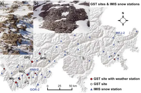
Figure 2 Ground surface temperature (GST) sites (circles) and Intercantonal Measurement and Information System (IMIS) snow stations (blue triangles) in the Swiss Alps. The photographs show typical, spatially heterogeneous snow conditions (a) along a wind-exposed mountain ridge in early winter and (b) in

early summer. Source background map: Federal Office of Topography. Thisfigure is available in colour online at wileyonlinelibrary.com/journal/ppp.

http://doc.rero.ch

maintained by SLF) were used for validation for the period between 1994 and 2015. IMIS stations record meteorologi- cal parameters such as snow depth and GST (at the ground surface) between 2000 and 3000 m asl in the Swiss Alps, but many of these stations are not located on permafrost (see Supplementary Material Table S1). The snow depth data from the IMIS stations are measured indirectly by ultra- sonic sensors, and raw data were used for this study. IMIS GST time series were pre-processed similar to those from PERMOS and the same aggregates were calculated.

Gridded AirT Data from MeteoSwiss

Because AirT is not measured at all PERMOS sites but is required to approximate SMRs, the gridded data product TabsD (2 km resolution based on ~ 90 stations in Switzerland) from MeteoSwiss has been used for daily mean AirT (Frei, 2014). Using these data and assuming a constant lapse rate of -0.0055°C m

, daily mean AirT time series were reconstructed for each of the GST loggers. The lapse rate was used to correct for the remaining elevation dif- ference between the closest grid cells (the overlapping cell and 8 surrounding cells were used) and the point of interest.

Validation with on-site AirT records from IMIS stations revealed a good agreement (R

: 0.98, root mean square error (RMSE): 1.56°C, p-value < 0.01, n: ~ 180 000 days) regarding daily mean values.

METHODS

The following procedures have been empirically developed on a large set of GST data in order to provide a robust and fl exible toolset applicable to different situations concerning data availability, quality and temporal resolution. The full documentation of the data processing can be found in the Supplementary Material including R code and a small sam- ple data-set.

Relationship between GST Variability and Snow Thermal Insulation

In mountainous areas such as the Swiss Alps, the daily SD of AirT ranges between 0.5 and 5°C with little sea- sonal differences. As long as the ground is not thermally insulated and remains dry, the daily SD of GST (GST

) is of the same order; values are slightly higher if recorded at ( ‘ skin surface temperature ’ ) or very close to the ground surface, and slightly lower if measured 10 – 20 cm below the surface. As Figure 3 illustrates, the presence of an insulating snow cover reduces GST

by a factor of at least fi ve to ten. Hence, semi-quantitative informa- tion on the thermal insulation effect of the snow cover and periods of phase change can be derived from short- term GST variations.

Figure 3 Seasonal patterns of air temperature (~ 2 m above the ground surface) and ground surface temperature (GST, ~ 20 cm below the surface) at the rock glacier Alpage de Mille (2400 m asl, MIL in Figure 2) over the period 1997–2014: (a, b) daily mean temperatures as well as average snow depth measured at a

nearby snow pole; (c, d) impact of the snow on the daily GST standard deviation.

http://doc.rero.ch

Detection of Zero Curtains, Basal Ripening and Snow Disappearance

During snow melt, GST should, theoretically, remain con- stantly at 0°C with short-term variations very close to ~ 0°C, because phase changes have the largest in fl uence on the GST signal. To account for the rather coarse thermal resolu- tion of some miniature temperature loggers (e.g. UTL-1 with

± 0.23 – 0.27°C), a threshold th

is set to 0.25°C. During pe- riods of phase change, absolute GST values will likely not sur- pass th

. Even if GST values fl uctuate between two values due to the limited thermal resolution of the sensors, GST

would still remain below half of th

. Based on GST

, we cal- culated GST

in running windows of 24 h aligned at the beginning (GST

) and end (GST

) of this pe- riod. Similarly, weekly SD (GST

, GST

) can be calculated from daily means. Accordingly, the zero curtain period (ZC) can be delineated as:

Or, if only daily mean GSTs are available, as:

Describing the start of the snow melt, the basal RD is arbitrarily de fi ned as the fi rst day which ful fi ls the criteria in Equations 1 or 2, respectively. Similarly, the SDD represents the fi rst day with positive GSTs following a continuous zero

curtain period. The successful detection of the RD is limited to locations and years displaying negative winter GSTs. A zero curtain period may occur during: (a) the melt of snow when the active layer is frozen (spring zero curtain); (b) the melt of fresh snow on still unfrozen ground (as often occurs in autumn);

(c) ground freezing; or (d) after rain-on-snow events when water percolates through the snowpack and refreezes at the bottom (Westermann et al., 2011; Wever et al., 2014).

Estimation of the Thermal Insulation Effect of the Snow and the Snow Onset

The difference between AirT and GST variations can be used to approximate such snow cover properties as the presence/absence of snow, snow thickness and timing of the snow melt (e.g. Hipp, 2012; Lewkowicz, 2008;

Lundquist and Lott, 2008; Schmid et al., 2012; Schmidt et al., 2009; Schneider et al., 2012; Tyler et al., 2008;

Apaloo et al., 2012). In contrast to previous work, the snow thermal insulation indices described hereafter classify dif- ferent levels of thermal insulation and delineate the start of the high-insulation period. In addition to the variability

snow

½ 0 ; …; 1 ¼

GSTSDweek

th1

þ 1

þ

þ 1

2 ∧ GST

≤ 0 : 5 (4)

ZC ¼

1 if j GST

j ≤ th

∧ GST

≤ th

2 ∨ GST

≤ th

2

0 if j GST

j> th

∨ GST

> th

2 ∨ GST

> th

2 8 >

> <

> >

:

(1)

ZC ¼

1 if GST

≤ th

∧ GST

≤ th

2 ∨ GST

≤ th

2

0 if GST

> th

∨ GST

> th

2 ∨ GST

> th

2 8 >

> <

> >

:

(2)

snow

½ 0 ; …; 1 ¼

GSTSDday

th1

þ 1

þ

þ 1

2 ∧ GST

≤ 1 (3)

http://doc.rero.ch

terms GST

(when analysing hourly data) and GST

(based on daily means), a GST-change term Δ GST

is used to describe the GST trend over one week.

Similar to the zero curtain detection, empirically de fi ned thresholds are used to distinguish between periods of higher and lower thermal insulation: th

is de fi ned as the 95th per- centile of GST

(or GST

, respectively) during January – March (when an insulating snow cover is most likely in the Swiss Alps) and is constrained to the value range 0.1 – 0.5. Likewise, the threshold th

is derived from the 95th percentile of Δ GST

and is constrained to the values 0.5 – 1.5. In other words, these thresholds represent values which are very unlikely to be surpassed if a thermally insulat- ing snow cover is present. The snow thermal indices snow

(based on hourly data) and snow

(based on daily means) consist of a SD and a Δ change term and are de fi ned as follows:

If GST

> th

, GST

> th

or Δ GST

> th

the respective term is set to 0, indicating no thermal insulation. If the respective thresholds are undercut, the indices become pos- itive and may approach the maximum value 1 when the vari- ability and Δ change term are equal to 0 (complete thermal insulation).

To account for site-speci fi c characteristics, such as the placement depth of the sensors, the exposure to solar radia- tion and wind, as well as the roughness and porosity of the ground material at the surface, th

and th

are de fi ned sepa- rately for each time series. The values obtained for th

were similar to short-term variations in GST representing snow- covered periods reported in other studies (Schmid et al., 2012; Schneider et al., 2012). To achieve comparable re- sults across different sites and years, both thresholds were constrained to a reasonable range of values. Δ GST

was introduced to address the weekly scale and potentially underestimated insulation when the GST values are fl uctuat- ing between two values due to limited thermal resolution.

The additional fi lter criteria using absolute GST

or GST

avoid scatter in summer and autumn, when small snow events may lead to a temporary thermal insulation (Hipp, 2012; Lewkowicz, 2008; Schmid et al., 2012). Capturing such short snow events is, however, not the aim of the indi- ces snow

and snow

. Snow

may be particularly suitable for time series with changing temporal resolution over time, or if only daily mean GST values are available. To remove spikes, both indices were additionally smoothed with a one week median fi lter.

To compare snow

and snow

, we adapted an algorithm proposed by Hipp (2012), originally developed for the auto- matic detection of snow depths from snow poles instru- mented with iButtons (Lewkowicz, 2008). This approach, here called snow

, estimates the thermal insulation effect of the snow cover based on the temperature variability above (AirT) and below (GST). It was modi fi ed using weekly SD (GST

, AirT

) instead of hourly vari- ance to preserve the units and to make its application possi- ble even if only daily means are available (cf. Equation 5).

Like snow

, snow

was also restricted to GST

≤ 0.5°C and smoothed with a weekly median fi lter.

snow

½ 0 ; …; 1 ¼ ð AirT

GST

Þ AirT

þ GST

ð Þ ∧ GST

≤ 0 : 5 (5) All three indices may be used to delineate periods of dif- fering thermal insulation, such as the fi rst day of positive snow indices in winter (SOD), or the fi rst day of a subse- quent period of high thermal insulation of at least 2 weeks with mean snow indices ≥ 0.5 (HTIstart).

Approximation of SMRs and Maximal Snow Depths Snow melt is primarily controlled by AirT and the radia- tion balance at the surface (Ohmura, 2001). Melting is further in fl uenced by the refreezing of meltwater within the snowpack and the percolation of rain and surface run- off into the snow (Pomeroy and Brun, 2001; Senese et al., 2014). Because point-speci fi c data on radiation, precipitation, snow density and albedo are usually lacking, only very simple models are suitable to quantify the snow melt in high-alpine terrains. AirT is the proxy of choice since it partly integrates many components of the energy balance and may be extrapolated over distances of 10 – 100 km with reasonable uncertainty (Tardivo and Berti, 2012;

Lang and Braun, 1990). Degree-day and energy balance ap- proaches approximating snow melt have been developed and successfully applied in hydrological modelling (Hock, 2003;

Lehning et al., 2006; Martinec, 1960) and glacier mass balance studies (Braithwaite and Zhang, 2000; Pellicciotti et al., 2005; Senese et al., 2014). However, the absolute accuracy of such a degree-day model is limited due to simpli fi cations (e.g. unknown snow density, neglected spatial patterns) and scale issues (Lang and Braun, 1990).

Reasonable values for the snow density ρ are required.

Jonas et al. (2009) found, from snow probings in the Swiss Alps, that ρ typically ranges between 300 and 500 kgm

between April and June. This is the period when snow melt occurs at PERMOS sites. SWE records obtained by Schmid et al. (2012) around Piz Corvatsch (eastern Switzerland) in March and April 2010 were of the same order (~360 kgm

some weeks before the snow melt started at high altitude).

Therefore, a bulk snow density of ~ 400 kgm

is assumed for permafrost areas in the Swiss Alps during the snow melt period, similar to values for old and wet snow (Judson and Doesken, 2000; Meløysund et al., 2007).

By coupling the point-speci fi c information on the timing of the melting period (zero curtain, cf. Equations 1 and 2) with positive daily AirT data (AirT

), the SWE of the maximal snow depth (hs) at the basal RD and daily SMRs can be approximated, speci fi cally for the points where GST is measured. The melt index (Equation 6) is a linear degree-day model based on AirT

using the factor A for calibration. A was chosen according to a study from Zingg (1951) on the Weiss fl uhjoch (WFJ-2 in Figure 2), which revealed strong agreement between AirT

and meltwater runoff measurements with A = 4.5. For example, an average melting day in early summer with

http://doc.rero.ch

an AirT

of 10°C would melt ~ 45 mm SWEs or ~ 11 cm of snow, respectively.

melt index SWE ½ ; mm ≅ Δ hs ρ Δ t ≅

A X

t¼RD

AirT

Δ t

(6) The approach is based on the assumption that the total amount of snow converted into water during a given time window is mainly related to the sum of AirT

within the same period.

VALIDATION

Validation of the Snow Thermal Indices

Because the snow indices characterise the thermal decoupling of the ground surface from variations in AirT but do not indicate snow depth, their validation can only be done qualitatively or by comparing snow insulation

classes and snow depth for speci fi c periods. For a fi rst visual comparison, all three snow indices (Equations 3 – 5) have been overlain with the GST and snow depth records from IMIS stations. As Figure 4 shows for station GOR-2, there are large seasonal and interannual variations in the timing and thickness of the snow cover. The snow indices seem capable of representing this behaviour, and the timing of the high-insulation period can be detected. Moreover, these examples show some typical problems: for the detection of the melting period (zero curtain, RD and SDD), well-calibrated GST input data are required. This explains why in 1996 the zero curtain period could not be automati- cally detected for GOR-2, because there was a small yet systematic GST offset. In 1995 and 1997, phase changes dominated the GST signal throughout winter. If GST warms very rapidly before the zero curtain, the snow indices may spontaneously drop. The snow indices peak during the melting period.

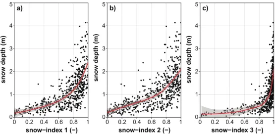
Monthly mean snow depths and snow indices are com- pared in Figure 5 for a second validation. Variations between snow-rich and snow-poor periods seem to be dis- tinguishable with all snow indices. However, snow

appears

Figure 4 Comparison of GST and the derived snow indices at the IMIS station GOR-2 for the past 20 years. The blue areas on top of the GST curves represent periods with zero curtains (Equation 1), and the grey-shaded areas at the bottom show the measured snow depth (m). The coloured lines are the GST-derived snow indices (Equations 3–5) indicated at the top of thefigure. Snow and IMIS-data © 2015, SLF. Thisfigure is available in colour online at wileyonlinelibrary.com/journal/ppp.

http://doc.rero.ch

to be much more sensitive to shallow snow depths < 50 cm, compared to snow

and snow

. The large scatter can be ex- plained by site-speci fi c and temporal differences in the ter- rain and snow characteristics. However, intermediate snow indices do not show a clear relation to respective snow depths (e.g. 20 – 50 cm) because very smooth surfaces may require up to 30 – 50 cm less snow than rough, coarse-blocky terrains to reach the same thermal insulation effect. Raw data for the IMIS stations were checked for plausible values but were not corrected. Overall, the snow indices indicate the general snow thermal characteristics of different years or locations.

Validation of the Snow Melt Index

The melt index (Equation 6) has been validated using IMIS data for ~ 500 melting periods. Cumulative SMR and cumula- tive snow depth loss (converted into SWEs using a bulk density of 400 kgm

) have been compared. As Figure 6 shows, this relationship is strong (R

: ~ 0.88) and nearly lin- ear. However, the compaction of the snow cover with time, spatio-temporal variance in global radiation, precipitation events during the melting period and the refreezing of meltwa- ter are not taken into account. Regarding the data obtained, the optimal value for A ranges between 3.5 and 5 depending on the station, but the average regression slope (~ 4.1) is close to the value of 4.5 as proposed by Zingg (1951).

Because the variance in AirT is the only proxy for all the processes in fl uencing snow melt, absolute SMR values require cautious interpretation. The largest uncertainty of this degree-day model relates to the snow density, which may vary up to ± 20 per cent, as well as the disregarded variance in global radiation. As long as relative values (e.g. differences between years) are compared, reliable results are expected, due to large interannual differences.

APPLICATION OF THE SNOW AND MELT INDI- CES ON GST MONITORING DATA

The snow and melt indices have been applied to GST mon- itoring time series from the Swiss Alps, and selected results are shown subsequently in order to illustrate the potential use in mountain permafrost research.

Figure 6 Validation of the melt index using the degree-day factorAof 4.5 (x-axis) with the respective cumulative snow depth loss (y-axis). Each data point represents the mean of one melting period (n = 495). The red line shows the best linearfit (slope of 4.1) the grey area represents the 95 per

cent regression confidence interval. Snow water equivalents (SWE, mm) have been approximated using a bulk snow density of 400 kgm^-3. IMIS

data © 2015, SLF. Thisfigure is available in colour online at wileyonlinelibrary.com/journal/ppp.

Figure 5 Comparison of (a–c) snow indices derived from GST data and snow depth observations recorded at 33 IMIS stations. Each point corresponds to the mean value of one month (n = 528, restricted to monthly mean GSTs≤-0.3°C). The red lines represent local polynomial regressionsfitted through the data with the corresponding 95 per cent confidence interval in grey. IMIS data © 2015, SLF. Thisfigure is available in colour online at wileyonlinelibrary.com/journal/ppp.

http://doc.rero.ch

Snow Onset and Thermal Insulation

The thermal insulation of the snowpack and the timing of the snow onset are important to the ground thermal re- gime of mountain permafrost, because they control the in- tensity of ground cooling over a long period of the year.

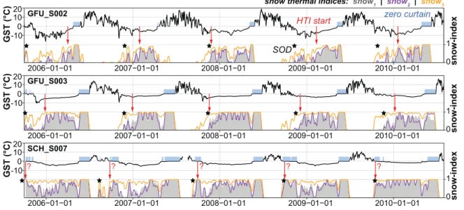
As Figure 7 shows, the differences in the thermal insula- tion by the snow cover can be very large even for adja- cent loggers: while logger GFU_S002 is situated on a ridge and exposed to wind, GFU_S003 is situated ~ 20 m away on the same landform but in a gully prone to snow accumulation. In consequence, at GFU_S002 the thermal insulation is clearly lower and the high thermal insulation period (HTIstart) starts later in the season, which results in more negative GST values during winter. The example from the Schilthorn (SCH_S007 in Figure 7) further shows that fi ne-grained subsurface materials are prone to zero cur- tain periods in autumn and spring, due to the increased moisture content (latent heat) and heat capacity of the (up- per) ground layers. In such situations, the HTIstart cannot be determined and the informative value of the snow indi- ces regarding the thermal insulation effect is limited. The spatial variability between the different loggers is largest in years with early HTIstart, while winter cooling peaks in years with late HTIstart.

Timing and Duration of the Melting Period

The timing of the snow melt (particularly SDD) greatly in fl uences the surface energy balance in early summer, resulting in up to 5 – 10°C difference between snow-free and the snow-covered locations, equalling an impact on the annual mean of 0.01 – 0.02°C per day. Regarding the

temporal evolution of the SDD, no clear trend has been observed during the past 15 years, although the interan- nual variations are considerable (SD: ± 20 days). The spa- tial variability of the SDD is even larger than the temporal variations, and some locations experiencing an early melt-out may be snow-free up to two months before the snow nearby is completely gone (Figures 2b, 4 and 7). The mean zero curtain duration (SDD-RD) for more than 1500 clearly identi fi able melting periods is 48 days (SD: ± 20 days). Such long zero curtains as well as the high spatial and temporal variability illustrate the in fl uence of snow on the local surface energy balance in early summer.

Estimated SWEs and SMRs

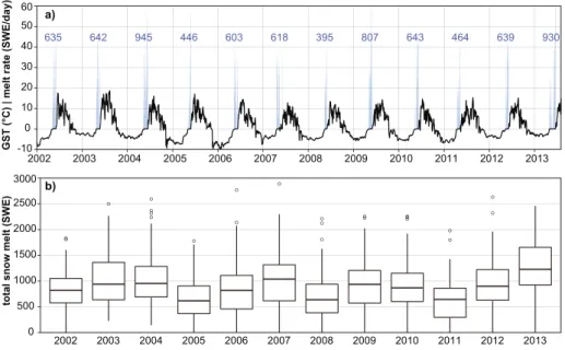
The application of the melt index using GST time series from PERMOS revealed large spatial and temporal vari- ability concerning daily SMRs. Figure 8 illustrates the temporal evolution of the SMR for one example, and sum- marises 74 complete GST time series from 11 sites for the period 2002 – 13. Similarly to the snow indices, consider- able interannual differences also appear regarding the SMR. The total sum of the SMR melted during the zero curtain ranges from nearly 0 to about 2500 mm (SWE).

The average value of the 840 melting periods analysed is 890 mm (SWE), equalling a thickness of ~ 2.2 m of snow at a density of 400 kgm

.

This simple approach seems capable of reproducing sea- sonal and interannual variations of the SMR that are close to natural variations. It achieves this in spite of the high un- certainty related to the assumption of the constant snow density, by neglecting the distinction between melt and sub- limation (Strasser et al., 2008) and disregarding the effects of radiation and the refreezing of water in the snowpack.

Figure 7 Comparison of GST and snow indices for selected GST time series from the sites Gemmi (GFU) and Schilthorn (SCH). Black lines: daily mean GST; blue areas: periods with phase change (zero curtains); grey areas: snow indexsnow1; purple lines:snow2; orange lines:snow3; black stars: snow onset date (SOD) based onsnow1; red arrows: start of the high-insulation winter period (HTIstart) based onsnow1.HTIstartmay occur at the same time as theSOD

or much later in the season. Thisfigure is available in colour online at wileyonlinelibrary.com/journal/ppp.

http://doc.rero.ch

One major bene fi t is its ability to extract SMR time series (or the cumulated snow melt), which is highly irregular at short timescales of days to weeks. While the SMR increases in June due to increased AirT (and high radiation), it dips be- low 1 mm SWE per day almost every third day.

DISCUSSION

Our snow indices contain semi-quantitative information on the thermal insulation effect of the snow, information which could not be directly extracted from snow depth records be- cause the thermal resistance of the snow layer depends on its density and structure as well as terrain characteristics.

The indices can also help reconstruct past snow thermal conditions using long-term GST monitoring data. To our knowledge, the snow indices are a unique approach to de- scribe the snow onset and the start of the high-insulation period in a systematic and standardised way. They also elu- cidate the spatio-temporal variability of snow characteristics in remote areas using miniature temperature loggers, which are well established in the permafrost community.

The validation of the snow indices, however, is demand- ing, and interpretation of the results requires expert knowledge of the local terrain and microclimate. In situa- tions with early snow fall, the HTIstart and the snow RD can be dif fi cult to delineate, particularly at locations with relatively warm or humid conditions because variations in the surface energy balance in the GST data may be masked by phase changes (Figures 4 – 7). Moreover, the density and structure of the snow as well as the amount of snow required for a given thermal insulation effect change throughout the

season, as the density increases 100 – 300 per cent from fresh snow to old and wet snow (Jonas et al., 2009). The thresh- old de fi nitions might require adaptation in order to apply the method to other climatic situations or using a different measurement setup for the GST data. The application using GST monitoring time series from the Swiss Alps showed that an insulating snow cover is present in the majority of cases, at least for some weeks each winter. However, the timing and duration of these high-insulation periods may vary greatly for different locations, sites and years. The po- tential absence or temporal shift of the high-insulation pe- riod implies that theoretical values which depend on the concept of thermal insulation in late winter, such as the base temperature of the winter snow cover (Haeberli, 1973) or the winter equilibrium temperature (Delaloye, 2004), may not be determined in all situations.

The melt index (which describes the SMR) agrees well with snow data from the IMIS stations using the degree- day factor A = 4.5 as proposed by Zingg (1951). Its applica- tion to GST monitoring data revealed promising new insights on the spatial and temporal variability of the melt- water released from the snowpack at the position of the GST loggers. The use of daily means seems appropriate be- cause A was also calibrated using daily means (Zingg, 1951), and the downscaling of point-speci fi c AirT values from gridded data or remote stations is supposed to be quite robust for daily means. For the Swiss Alps, the gridded daily mean AirT from MeteoSwiss agree closely with obser- vations from the IMIS stations. These gridded data facilitate the processing of the melt index for numerous sites when on-site AirT observations are lacking. The key use of the melt index will probably be in the analysis of rock glacier kinematics, where clear relationships between annual

Figure 8 Snow melt rates (SMR) for GST locations derived from Equation 6: (a) daily mean GST (black) andSMRfor logger MIL_S005 (MIL on Figure 2).

The numbers in blue indicate the total snow water equivalents (SWE, mm) melted during the zero curtain. In (b) interannual variations of the total SWE melted during the zero curtain are shown for 12 years based on 74 loggers with complete data from 11 different study sites. On average, total SWE is about 890 mm, which equals ~ 2.2 m of snow assuming a bulk snow density of 400 kgm^-3. Thisfigure is available in colour online at wileyonlinelibrary.com/journal/ppp.

http://doc.rero.ch

displacement rates and GST variations have been found (Delaloye et al., 2010), but the role of the meltwater in fi ltra- tion is still not suf fi ciently understood. To make the melt in- dex physically more consistent, the bulk snow density function applied by Jonas et al. (2009) could be integrated, or an explicit radiation component could be in- troduced if such data are available.

CONCLUSIONS AND OUTLOOK

Our new data processing techniques quantify the thermal insulation effect of the snow cover on the ground and de- lineate periods of high thermal insulation and snow melt, as well as the SMR during zero curtain periods in spring.

The algorithms are designed for permafrost conditions using GST data and were validated with fi eld data from snow stations in the Swiss Alps. Potential applications of the indices may characterise snow thermal insulation and the SMR for different locations and years. However, the threshold de fi nitions and the degree-day factor should be adapted before applying the indices to other regions

with differing climate, snow and ground properties. The snow indices might be used as an additional validation parameter to assess the representation of upper boundary conditions in permafrost models (Gisnås et al., 2014;

Staub et al., 2015).

ACKNOWLEDGEMENTS

We gratefully acknowledge the Swiss National Science Foun- dation for funding of the Sinergia project The Evolution of Mountain Permafrost in Switzerland (TEMPS, no. CRSII2 136279) as well as PERMOS and our colleagues within TEMPS for providing observational data. Special thanks go to Dragan Vogel for his valuable advice on the signal processing of GST time series, and to Brianna Rick for proofreading the English. Moreover, we would like to thank the Editor, Julian Murton, as well as two anonymous referees for their detailed and helpful comments and suggestions. IMIS snow station data were kindly provided by the WSL Institute for Snow and Ava- lanche Research SLF, and gridded AirT data by the Federal Of fi ce for Meteorology and Climatology MeteoSwiss.

REFERENCES

Apaloo J, Brenning A, Bodin X. 2012. Interac- tions between seasonal snow cover, ground surface temperature and topography (Andes of Santiago, Chile, 33.5°S).Permafrost and Periglacial Processes 23: 277–291. DOI:

10.1002/ppp.1753.

Braithwaite RJ, Zhang Y. 2000. Sensitivity of mass balance offive Swiss glaciers to tempera- ture changes assessed by tuning a degree-day model.Journal of Glaciology46: 7–14. DOI:

10.3189/172756500781833511.

Delaloye R. 2004. Contribution à l’étude du pergélisol de montagne en zone marginale.

PhD thesis, Department of Geosciences, University of Fribourg, GeoFocus No. 10.

Delaloye R, Lambiel C, Gärtner-Roer I. 2010.

Overview of rock glacier kinematics research in the Swiss Alps.Geographica Helvetica 65: 135–145. DOI:10.5194/gh-65-135-2010.

Frei C. 2014. Interpolation of temperature in a mountainous region using nonlinear profiles and non-Euclidean distances.International Journal of Climatology 34: 1585–1605.

DOI:10.1002/joc.3786.

Gisnås K, Westermann S, Schuler TV, Litherland T, Isaksen K, Boike J, Etzelmüller B. 2014. A statistical approach to represent small-scale variability of per- mafrost temperatures due to snow cover.

The Cryosphere 8: 2063–2074. DOI:10.

5194/tc-8-2063-2014.

Goodrich LE. 1982. The influence of snow cover on the ground thermal regime.Cana- dian Geotechnical Journal 19: 421–432.

DOI:10.1139/t82-047.

Haeberli W. 1973. Die Basis-Temperatur der winterlichen Schneedecke als möglicher Indikator für die Verbreitung von Permafrost in den Alpen.Zeitschrift für Gletscherkunde und Glazialgeologie9: 221–227.

Hanson S, Hoelzle M. 2005. Installation of a shallow borehole network and monitoring of the ground thermal regime of a high alpine discontinuous permafrost environ- ment, Eastern Swiss Alps. Norsk Geografisk Tidsskrift - Norwegian Journal of Geography 59: 84–93. DOI:10.1080/

00291950510020664.

Hipp T. 2012. Mountain Permafrost in Southern Norway: Distribution, Sparial Variability and Impacts of Climate Change.

PhD thesis, Faculty of Mathematics and Natural Science, University of Oslo.

Hock R. 2003. Temperature index melt model- ling in mountain areas.Journal of Hydrol- ogy 282: 104–115. DOI:10.1016/S0022- 1694(03)00257-9.

Hoelzle M, Wegmann M, Krummenacher B.

1999. Miniature temperature dataloggers for mapping and monitoring of permafrost in high mountain areas: first experience from the Swiss Alps. Permafrost and Periglacial Processes 10: 113–124. DOI:

10.1002/(SICI)1099-1530(199904/06)10:

2<113::AID-PPP317>3.0.CO;2-A.

Hoelzle M, Mittaz C, Etzelmüller B, Haeberli W. 2001. Surface energy fluxes and distribution models of permafrost in European mountain areas: an overview of current developments. Permafrost and Periglacial Processes 12: 53–68. DOI:10.

1002/ppp.385.

Hüsler F, Jonas T, Riffler M, Musial JP, Wunderle S. 2014. A satellite-based snow cover climatol- ogy (1985-2011) for the European Alps derived from AVHRR data.The Cryosphere 8: 73–90. DOI:10.5194/tc-8-73-2014.

Isaksen K, Hauck C, Gudevang E, Ødegård RS, Sollid JL. 2002. Mountain permafrost distribution in Dovrefjell and Jotunheimen, southern Norway, based on BTS and DC resistivity tomography data. Norsk Geografisk Tidsskrift - Norwegian Journal of Geography56: 122–136. DOI:10.1080/

002919502760056459.

Isaksen K, Ødegård RS, Etzelmüller B, Hilbich C, Hauck C, Farbrot H, Eiken T, Hygen HO, Hipp TF. 2011. Degrading Mountain Permafrost in Southern Norway:

Spatial and Temporal Variability of Mean Ground Temperatures, 1999-2009.Perma- frost and Periglacial Processes 22:

361–377. DOI:10.1002/ppp.728.

Ishikawa M. 2003. Thermal regimes at the snow–ground interface and their implica- tions for permafrost investigation.Geomor- phology52: 105–120. DOI:10.1016/S0169- 555X(02)00251-9.

Jonas T, Marty C, Magnusson J. 2009. Esti- mating the snow water equivalent from snow depth measurements in the Swiss Alps.Journal of Hydrology378: 161–167.

DOI:10.1016/j.jhydrol.2009.09.021.

Judson A, Doesken N. 2000. Density of Freshly Fallen Snow in the Central Rocky Mountains. Bulletin of the American Meteorological Society 81:

1577–1587. DOI:10.1175/1520-0477 (2000)081<1577:DOFFSI>2.3.CO;2.

http://doc.rero.ch

Keller F, Gubler H. 1993. Interaction between snow cover and high mountain permafrost, Murtèl-Corvatsch, Swiss Alps. InProceed- ings of the 6th International Conference on Permafrost, Brown J, French H.M., Grave N.A., Guodong C., King L., Koster E.A., Péwé T.L. (eds). South China Univer- sity of Technology Press: Wushan Guang- zhou China; 332–337.

Lang H, Braun L. 1990. On the information content of air temperature in the context of snow melt estimation.Hydrology of Moun- tainous Areas. Proceedings of the Strbské Pleso Workshop, Czechoslovakia, June 1988. IAHS Publ. no190: 347–354.

Laternser M, Schneebeli M. 2003. Long-term snow climate trends of the Swiss Alps (1931-99).International Journal of Clima- tology23: 733–750. DOI:10.1002/joc.912.

Lehning M, Völksch I, Gustafsson D, Nguyen TA, Stähli M, Zappa M. 2006. ALPINE3D:

a detailed model of mountain surface processes and its application to snow hydrology. Hydrological Processes 20:

2111–2128. DOI:10.1002/hyp.6204.

Lewkowicz AG. 2008. Evaluation of Minia- ture Temperature-loggers to Monitor Snow- pack Evolution at Mountain Permafrost Sites, Northwestern Canada. Permafrost and Periglacial Processes 19: 323–331.

DOI:10.1002/ppp.625.

Luetschg M, Lehning M, Haeberli W. 2008. A sensitivity study of factors influencing warm/thin permafrost in the Swiss Alps.

Journal of Glaciology54: 696–704. DOI:

10.3189/002214308786570881.

Lundquist JD, Lott F. 2008. Using inexpen- sive temperature sensors to monitor the du- ration and heterogeneity of snow-covered areas.Water Resources Research44: 1–6.

DOI:10.1029/2008WR007035.

Marmy A, Salzmann N, Scherler M, Hauck C.

2013. Permafrost model sensitivity to sea- sonal climatic changes and extreme events in mountainous regions.Environmental Re- search Letters 8: 035048. DOI:10.1088/

1748-9326/8/3/035048.

Martinec J. 1960. The degree-day factor for snowmelt-runoff forecasting. IUGG Gen- eral Assembly of Helsinki, IAHS Commis- sion of Surface Waters, IAHS Publ. no.

51: 468–477.

Meløysund V, Leira B, Høiseth KV, Lisø KR.

2007. Predicting snow density using

meteorological data.Meteorological Appli- cations14: 413–423. DOI:10.1002/met.40.

Noetzli J, Gruber S. 2005. Alpiner Permafrost - ein Überblick. In Jahrbuch des Vereins zum Schutz der Bergwelt, Lintzmeyer K (ed),70. Selbstverlag: München; 111–121.

Ohmura A. 2001. Physical Basis for the Temperature-Based Melt-Index Method.

Journal of Applied Meteorology 40:

753–761. DOI:10.1175/1520-0450(2001)040<

0753:PBFTTB>2.0.CO;2.

Outcalt SI, Nelson FE, Hinkel KM. 1990. The zero-curtain effect: Heat and mass transfer across an isothermal region in freezing soil.

Water Resources Research26: 1509–1516.

DOI:10.1029/WR026i007p01509.

Pellicciotti F, Brock B, Strasser U, Burlando P, Funk M, Corripio J. 2005. An enhanced temperature-index glacier melt model including the shortwave radiation balance:

development and testing for Haut Glacier d’Arolla, Switzerland. Journal of Glaciology 51: 573–587. DOI:10.3189/

172756505781829124.

PERMOS. 2013. Permafrost in Switzerland 2008/2009 and 2009/2010, Noetzl J (ed).

Glaciological Report Permafrost No. 10/11 of the Cryospheric Commission of the Swiss Academy of Sciences, Zurich, Switzerland.

Pomeroy JW, Brun E. 2001. Physical proper- ties of snow. InSnow Ecology: An Interdis- ciplinary Examination of Snow-covered Ecosystems, Jones HG, Pomeroy JW, Walker DA, Hoham RW (eds). Cambridge University Press: Cambridge; 45–118.

Schmid MO, Gubler S, Fiddes J, Gruber S.

2012. Inferring snowpack ripening and melt-out from distributed measurements of near-surface ground temperatures. The Cryosphere 6: 1127–1139. DOI:10.5194/

tc-6-1127-2012.

Schmidt S, Weber B, Winiger M. 2009. Analyses of seasonal snow disappearance in an alpine valley from micro- to meso-scale (Loetschental, Switzerland). Hydrological Processes 23:

1041–1051. DOI:10.1002/hyp.7205.

Schneider S, Hoelzle M, Hauck C. 2012. Influ- ence of surface and subsurface heterogene- ity on observed borehole temperatures at a mountain permafrost site in the Upper Engadine, Swiss Alps. The Cryosphere6:

517–531. DOI:10.5194/tc-6-517-2012.

Senese A, Maugeri M, Vuillermoz E, Smiraglia C, Diolaiuti G. 2014. Using daily

air temperature thresholds to evaluate snow melting occurrence and amount on Alpine glaciers by T-index models: the case study of the Forni Glacier (Italy). The Cryosphere 8: 1921–1933. DOI:10.5194/

tc-8-1921-2014.

Staub B, Marmy A, Hauck C, Hilbich C, Delaloye R. 2015. Ground temperature var- iations in a talus slope influenced by perma- frost: a comparison of field observations and model simulations. Geographica Helvetica 70: 45–62. DOI:10.5194/gh-70- 45-2015.

Stocker-Mittaz C, Hoelzle M, Haeberli W.

2002. Modelling alpine permafrost distribu- tion based on energy-balance data: a first step.Permafrost and Periglacial Processes 13: 271–282. DOI:10.1002/ppp.426.

Strasser U, Bernhardt M, Weber M, Liston GE, Mauser W. 2008. Is snow sublimation important in the alpine water balance?The Cryosphere 2: 53–66. DOI:10.5194/tc-2- 53-2008.

Tardivo G, Berti A. 2012. A Dynamic Method for Gap Filling in Daily Temperature Datasets.Journal of Applied Meteorology and Climatology51: 1079–1086. DOI:10.

1175/JAMC-D-11-0117.1.

Tyler SW, Burak SA, McNamara JP, Lamontagne A, Selker JS, Dozier J. 2008.

Spatially distributed temperatures at the base of two mountain snowpacks measured with fiber-optic sensors. Journal of Glaciology 54: 673–679. DOI:10.3189/

002214308786570827.

Westermann S, Boike J, Langer M, Schuler TV, Etzelmüller B. 2011. Modeling the im- pact of wintertime rain events on the ther- mal regime of permafrost.The Cryosphere 5: 945–959. DOI:10.5194/tc-5-945-2011.

Wever N, Jonas T, Fierz C, Lehning M. 2014.

Model simulations of the modulating effect of the snow cover in a rain-on-snow event.Hy- drology and Earth System Sciences 18:

4657–4669. DOI:10.5194/hess-18-4657-2014.

Zhang T. 2005. Influence of the seasonal snow cover on the ground thermal regime: An overview. Reviews of Geophysics 43:

RG4002. DOI:10.1029/2004RG000157.

Zingg T. 1951. Beziehung zwischen Temperatur und Schmelzwasser und ihre Bedeutung für Niederschlags- und Abflussfragen. IUGG General Assembly of Bruxelles, IAHS Publ.

no.33: 266–269.

SUPPORTING INFORMATION

Additional supporting information may be found in the online version of this article at the publisher ’ s web site.

http://doc.rero.ch