HAL Id: hal-02323430
https://hal.archives-ouvertes.fr/hal-02323430
Submitted on 21 Oct 2019
HAL is a multi-disciplinary open access
archive for the deposit and dissemination of
sci-entific research documents, whether they are
pub-lished or not. The documents may come from
teaching and research institutions in France or
abroad, or from public or private research centers.
L’archive ouverte pluridisciplinaire HAL, est
destinée au dépôt et à la diffusion de documents
scientifiques de niveau recherche, publiés ou non,
émanant des établissements d’enseignement et de
recherche français ou étrangers, des laboratoires
publics ou privés.
determinations
Sylvain Dupont, J-L Rajot, M. Labiadh, G. Bergametti, S. Alfaro, C. Bouet,
R. Fernandes, B. Khalfallah, E. Lamaud, B. Marticoréna, et al.
To cite this version:
Sylvain Dupont, J-L Rajot, M. Labiadh, G. Bergametti, S. Alfaro, et al.. Aerodynamic parameters
over an eroding bare surface: reconciliation of the law of the wall and eddy covariance determinations.
Journal of Geophysical Research: Atmospheres, American Geophysical Union, 2018, 123 (9),
pp.4490-4508. �10.1029/2017JD027984�. �hal-02323430�
Aerodynamic Parameters Over an Eroding Bare
Surface: Reconciliation of the Law of the Wall
and Eddy Covariance Determinations
S. Dupont1 , J-L. Rajot2,3,4 , M. Labiadh3, G. Bergametti4 , S. C. Alfaro4, C. Bouet2,4 ,
R. Fernandes1 , B. Khalfallah4, E. Lamaud1, B. Marticorena4 , J-M. Bonnefond1, S. Chevaillier4,
D. Garrigou1, T. Henry-des-Tureaux2, S. Sekrafi3, and P. Zapf4
1ISPA, INRA, Bordeaux Sciences Agro, Villenave d’Ornon, France,2iEES Paris (Institut d’Ecologie et des Sciences de
l’Environnement de Paris), UMR IRD 242, Université Paris Est Créteil-Sorbonne Université-CNRS-INRA-Université Paris Diderot, Bondy, France,3IRA-Médenine, Médenine, Tunisia,4LISA (Laboratoire Interuniversitaire des Systèmes
Atmosphériques), UMR CNRS 7583, Universités Paris Est Créteil et Paris Diderot, IPSL, Créteil, France
Abstract
Assessing accurately the surface friction velocity is a key issue for predicting and quantifying aeolian soil erosion. This is usually done either indirectly from the law of the wall (LoW) of the mean wind velocity profile or directly from eddy covariance (EC) of the streamwise and vertical wind velocity fluctuations. However, several recent experiments have reported inconsistency between friction velocities deduced from both methods. Here we reinvestigate the determination of aerodynamic parameters (friction velocity and surface roughness length) over an eroding bare surface and look at the possible reasons for observing differences on these parameters following the method. For that purpose a novel field experiment was performed in South Tunisia under the research program WIND-O-V (WIND erOsion in presence of sparse Vegetation). We find no significant difference between friction velocities obtained from both law of the wall and EC approaches when the friction velocity deduced from the EC method was extrapolated to the surface. Surface roughness lengths show a clear increase with wind erosion, with more scattered values when deduced from the EC friction velocity. Our measurements further suggest an average value of the von Karman constant of 0.407±0.002, although individual wind events lead to different average values due probably to the definition of the ground level or to the stability correction. Importantly, the von Karman constant was found independent of the wind intensity and thus of the wind soil erosion intensity. Finally, our results lead to several recommendations for estimating the aerodynamic parameters over bare surface in order to evaluate saltation and dust fluxes.1. Introduction
The friction velocity u∗(or shear velocity) is one of the primary scaling parameters involved in aeolian soil ero-sion. It represents a velocity scale characterizing the surface wind shear stress. Under high-Reynolds-number flow, the surface wind shear induces mechanically turbulent eddies, which are responsible under strong wind for sediment entrainment and turbulent dispersal of dust in the lower atmosphere. As a consequence, exist-ing parameterizations of saltation and dust fluxes usually scale as the second or third power of u∗, and the initiation of soil erosion is defined from a threshold friction velocity above which erosion starts (e.g., Bagnold, 1941; Shao, 2008). Additionally, dust fluxes are usually estimated from the flux-gradient relationship, which also depends on u∗through the diffusion coefficient (e.g., Gillette et al., 1972). Hence, an accurate estimation of u∗is crucial in order to compare erosion flux parameterizations obtained from different field or laboratory experiments or to quantify accurately dust fluxes in field experiments.
The friction velocity has been often estimated indirectly by the erosion community from the law of the wall (LoW) approach, that is, the mean wind velocity profile within the surface layer (e.g., Marticorena et al., 2006; Shao et al., 2011). The LoW states that this velocity profile has a logarithmic form, or pseudo logarithmic for nonneutral thermal stratification, where the von Karman constant (𝜅) relates the surface wind shear stress to the near-surface wind velocity profile (Andreas et al., 2006). This indirect evaluation of u∗was justified by the use of cup anemometers measuring wind speed at low frequency (<1 Hz). Hence, most wind erosion
RESEARCH ARTICLE
10.1029/2017JD027984
Key Points:
• Conversely to previous studies, friction velocities obtained from the law of the wall and eddy covariance approaches are found similar • The von Karman’s constant is found
independent of wind soil erosion intensity
• Several recommendations are proposed to estimate aerodynamic parameters over bare surface in order to evaluate saltation and dust fluxes
Correspondence to: S. Dupont,
sylvain.dupont@inra.fr
Citation:
Dupont, S., Rajot, J-L., Labiadh, M., Bergametti, G., Alfaro, S. C., Bouet, C., et al. (2018). Aerodynamic parameters over an eroding bare surface: Rec-onciliation of the law of the wall and eddy covariance determina-tions. Journal of Geophysical Research:
Atmospheres, 123, 4490–4508.
https://doi.org/10.1029/2017JD027984
Received 30 OCT 2017 Accepted 3 APR 2018
Accepted article online 16 APR 2018 Published online 10 MAY 2018
©2018. American Geophysical Union. All Rights Reserved.
flux parameterizations derived from field experiments have been deduced from an indirect evaluation of u∗, assuming𝜅 = 0.40 or 0.41 (Li et al., 2010).
Nowadays, the more affordable access to high-frequency anemometers (≥10 Hz) has led to a growing number of field experiments where u∗is estimated directly from the correlations between the measured horizontal and vertical wind velocity fluctuations, also known as the eddy covariance (EC) approach, without requiring any assumption on the value of𝜅 and on the state of the atmosphere (e.g., Li et al., 2010; Lee & Baas, 2016). This direct evaluation of u∗is often considered as more reliable than the LoW approach. However, the direct evalu-ation of u∗from a single-height measurement without controlling for the presence of a constant momentum flux layer may be critical (Lee & Baas, 2016).
The few comparisons presented in the literature on the friction velocity obtained from the above direct and indirect methods were unsuccessful (e.g., Biron et al., 2004; King et al., 2008; Li et al., 2010; Lee & Baas, 2016). They all reported differences of more than 20 to 35% on u∗. No clear explanations were reported in these studies to explain these significant differences in u∗evaluation. Li et al. (2010) justified this difference from a modification of the von Karman constant in presence of windblown particles, while Lee and Baas (2016) observed later no link between the magnitude of their u∗difference and the presence of windblown parti-cles, which contradicts a modification of the𝜅 value. These latter authors suggested that u∗obtained from the logarithmic wind profile is more representative of a flow ensemble while u∗obtained from eddy covariance is more impacted by coherent eddy structures. This questions the range of eddy scales that should be consid-ered in u∗determination. Hence, an accurate evaluation of u∗appears problematic, while a precise value of u∗is crucial for establishing universal parameterizations of erosion fluxes or estimating dust fluxes.
The von Karman constant used in the LoW has been debated for years by the meteorological and fluid mechanic communities regarding its value and its constancy. Most of the studies suggest that𝜅 ranges from 0.35 to 0.45 (Högström, 1985; Oncley et al., 1996). The most recent study performed from field measurements in the atmospheric surface layer indicated a value closer to 0.37 than the usual values of 0.40–0.41 (Andreas et al., 2006), but with always a large variability of values around the mean due to measurement uncertainty. Frenzen and Vogel (1995) and Oncley et al. (1996) suggested that𝜅 is a function of the roughness Reynolds number (Re∗= u∗z0∕𝜈, where z0is the surface roughness length and𝜈 the fluid kinematic viscosity). However, later, Andreas et al. (2006) showed that this dependence on Re∗was due to an artificial correlation from shared variables used in the calculation of𝜅 and Re∗. In presence of aeolian soil erosion, the constant value of𝜅 has been questioned. Li et al. (2010) observed values of𝜅 decreasing with increasing soil erosion by wind. They found values as low as 0.264. By analogy with previous hydrodynamic research on river flow with suspended particles (e.g., Wright & Parker, 2004), they explained this decrease by the presence of saltating particles. Following these authors, in addition to increasing the surface roughness, the vertical concentration gradi-ent of saltating particles may also increase the velocity gradigradi-ent by damping the turbulence, leading to an “apparent” von Karman parameter. Since𝜅 intervenes in the evaluation of u∗from the LoW approach, uncer-tainty or modification of the value of𝜅 could significantly impact the value of u∗and could explain differences observed with the direct estimation of u∗.
Previous field experiments comparing LoW and EC approaches faced the absence of a constant flux layer and neglected stability correction in the LoW. Lee and Baas (2016) never observed a constant flux layer with height, and Li et al. (2010) were unable to verify its existence due to a single-height high-frequency anemometer. Both studies also neglected the stability correction of the LoW wind velocity profile, while the stability correction may be significant for assessing aerodynamic parameters, even in near-neutral conditions. These limitations could explain some of the discrepancies observed between LoW and EC approaches on the determination of the friction velocity and cancel the apparent decrease of the von Karman constant𝜅 with aeolian soil erosion suggested by Li et al. (2010).
This study ambitions to reconcile the determination of aerodynamic parameters (u∗and z0) from both, LoW and EC approaches, over an eroding bare surface. The main goal is to investigate the possible reasons for observing differences in aerodynamic parameters between both approaches such as the state of the con-stant flux layer, the value of the von Karman concon-stant, the stability correction, or the impact of soil erosion, in order to suggest recommendations for evaluating saltation and dust fluxes. For that purpose, a novel field experiment was performed in South Tunisia under the research program WIND-O-V (WIND erOsion in pres-ence of sparse Vegetation), where wind velocity and turbulpres-ence were measured at several heights using
vertical profiles of both cup and sonic anemometers. This experimental design allowed us to acquire wind velocity and friction velocity profiles, to compare u∗and z0obtained from both EC and LoW approaches, and to estimate𝜅.
2. Background
In atmospheric surface layers, the logarithmic region of the wind velocity above a bare surface starts around a few millimeters height. This logarithmic region is located above the buffer layer that marks the transition between the viscous layer at the surface and the turbulent layer above. During an erosion event, the pres-ence of saltating particles near the surface shifts the logarithmic layer to the upper saltation layer as saltating particles absorb momentum from the wind flow. The top of the logarithmic region depends on the extent of the surface. For a homogeneous and infinite surface, the top layer reaches a few hundred meters height in near-neutral conditions, while for limited surface extent the top layer matches the depth of the internal boundary layer developing from the upwind edge of the surface of interest (e.g., Kaimal & Finnigan, 1994). In the logarithmic region, the mean wind velocity profile is expressed as
⟨u(z)⟩ =u∗0 𝜅 [ log ( z z0 ) − Ψm (z L ) + Ψm( z0 L )] , (1)
where the symbol⟨⟩ denotes the time average, z is the vertical coordinate, u∗0is the friction velocity at the sur-face, Ψmis the stability function accounting for the thermal stratification of the surface layer (e.g., Högström, 1988), and L is the Monin-Obukhov length that compares the turbulence generated by buoyancy and wind shear. During wind erosion, (1) u∗0accounts for both surface wind shear and momentum flux absorbed by near-surface saltating particles (e.g., Raupach, 1991) and (2) z0 is known as the saltation roughness length, integrating the surface roughness length and the additional roughness induced by saltating particles (Owen, 1964).
With the LoW approach, u∗0is deduced indirectly from the linear regression of⟨u⟩, usually taking 𝜅 = 0.40 and knowing L independently. By neglecting Ψm(z0∕L), the linear regression of equation (1) leads to
⟨u(z)⟩ = A[log(z) − Ψm (z
L
)]
+ B, (2)
where A and B are the slope and intercept of the regression, respectively. Hereafter, the friction velocity deduced from this approach will be referred to as u∗0LoW. Hence, u∗0LoW = 𝜅A. If L is unknown (not in this study), an iterative procedure is usually performed to deduce u∗0,𝜃∗0(surface temperature scale) and z0from wind velocity and air temperature profiles (e.g., Frangi & Richard, 2000; Marticorena et al., 2006). The surface roughness length z0LoWis deduced from the slope A and intercept B of the regression, independently of𝜅: z0LoW= exp (−B∕A).
With the EC approach, the local friction velocity u∗(z) is estimated directly at the heights of the sonic anemometers from the correlations between the horizontal and vertical wind velocity fluctuations such as
u∗= (
⟨u′w′⟩2
+⟨v′w′⟩2)1∕4
, where the prime denotes the deviation from the averaged value and u, v, and w are the streamwise, spanwise, and vertical wind velocity components, respectively. In an ideal surface layer, the shear stress (or momentum flux) is constant with height, leading to u∗0 = u∗. However, in a real atmo-spheric surface layer, it is often difficult to observe a perfect constant flux layer (Andreas et al., 2006; Haugen et al., 1971; Högström, 1985). A surface friction velocity comparable to u∗0LoWis then deduced by extrapolat-ing the vertical distribution of u∗(z) to the surface (Biron et al., 2004). A linear extrapolation is often used such as (Andreas et al., 2006)
u∗(z) = az + u∗0. (3)
In an ideal surface layer the slope a would be zero. Hereafter, the friction velocity deduced at the surface (z = 0) from this approach will be referred to as u∗0EC. The surface roughness length z0ECis deduced from the intercept B of the regression of⟨u⟩ knowing u∗0ECand considering𝜅 = 0.40: z0EC = exp
(
−𝜅B∕u∗0EC). This represents the only way to estimate the roughness length from u∗0EC.
A direct estimation of u∗0allows us to evaluate the von Karman constant from the logarithmic form of the wind velocity profile. Hence,𝜅 can be deduced from the slope A of the regression of ⟨u⟩ knowing u∗0EC:𝜅 = u∗0EC∕A.
3. The WIND-O-V’s 2017 Experiment
3.1. Site
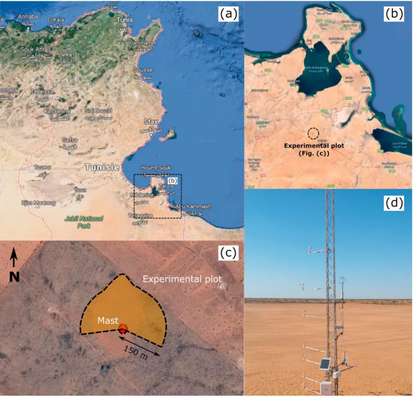
The WIND-O-V’s 2017 experiment took place from 1 March to 15 May 2017 in South Tunisia, in the experimen-tal range (Dar Dhaoui) of the Institut des Régions Arides of Médenine close to Médenine/Zarzis (Figures 1a and 1b). The site approximates a flat half-circle plot of 150-m radius where measurements were performed at the center of the circle in order to ensure a fetch of at least 150 m for westerly, northerly to easterly winds (Figure 1c). In the north, the fetch was slightly longer, about 200 m. The ground surface was flat with a slope less than 0.3∘ (0.6%) in all directions. The plot was surrounded by small bushes in the northwest (0.34±0.08-m height and 0.58 ± 0.20-m diameter) and young olive trees arranged in a square pattern (about 1.7 ± 0.3-m height, 1.5 ± 0.4-m diameter, and 26 m spaced) in the northeast. The soil is typical of the Jeffara basin with a loamy sand layer very prone to wind erosion. Before the experiment, the surface had been tilled with a disk plough and leveled with a wood board in order to meet the conditions of an ideal flat bare soil without soil crust or ridges.
3.2. Measurements
A 9-m high lattice mast was erected at the center of the half-circle plot (Figure 1d). The mast was well anchored in the ground to remove any possibility of mast motion with wind. On this mast, turbulent velocity compo-nents and air temperature fluctuations were measured simultaneously at 1.0, 1.9, 3.0, and 4.1 m above the sur-face using four ultra sonic anemometers (one Campbell Scientific CSAT3, two Gill R3, and one Gill WindMaster) sampling at 60, 50, 50, and 20 Hz, respectively. These four sonic anemometers allowed us in particular to estimate a vertical profile of friction velocities and thus to verify the presence of a constant flux layer. On the same mast, seven cup anemometers (0.2, 0.6, 1.3, 1.8, 3.0, 4.0, and 5.2 m) and four thermocouples (0.4, 1.6, 3.7, and 5.0 m) were also installed to measure simultaneously at 0.1 Hz the mean horizontal wind velocity and temperature profiles, respectively. These additional anemometers were used to characterize the logarithmic wind profile. Sonic anemometers were oriented toward the north and cup anemometers toward the northwest. All anemometers on the tower were intercalibrated prior to the experiment.
Among several instrumentations installed on the site for characterizing saltation and dust fluxes, one vertical array of five sediment traps like Big Spring Number Eight (BSNE) (Fryrear, 1986) was deployed to quantify the saltation flux, and two Saltiphones (Eijkelkamp®, Giesbeek, the Netherlands) were positioned close to the sur-face (about 7-cm height) and near the mast to follow at 0.1 Hz the dynamics of erosion events (beginning, end, and intensity). The principle of the Saltiphone is to count the impacts of saltating particles on a microphone surface (Spaan & Van den Abeele, 1991). The sediment traps had 0.10 m and 0.05 m horizontal and vertical openings, respectively, and were positioned vertically at 0.10, 0.25, 0.40, 0.60, and 0.90 m above the surface (using the middle of the opening as a reference). For this study, we focus solely on data from both BSNE and Saltiphones to identify the periods of aeolian soil erosion and to quantify the related windblown sediment fluxes, respectively.
3.3. Data Processing
A 15-min averaging time was chosen for computing all statistics characterizing the wind dynamics. This value was deduced from the point of convergence of the cumulative u-w cospectrum to an asymptote (Oncley et al., 1996). Figure 2 presents the average ogives Oguwof the momentum flux⟨u′w′⟩ obtained from the four sonic anemometers during three wind erosion events. As a reminder, Oguwis the cumulative integral of the u-w cospectrum Suw: Oguw(f ) =∫
f
∞Suw(s)ds, where the integration starts from the highest frequencies and f is the frequency. For all events, the four ogives converge nicely to 1 around fz∕⟨u⟩ ≈ 5×10⁻⁴, which corresponds to 15 min. This averaging time ensures that (1) all significant turbulent structures carrying momentum flux are included in the statistics and (2) estimated first- and second-order statistical moments reach reasonable uncer-tainty levels (see Appendix A). Considering a lower averaging time would underestimate the momentum flux, and thus the friction velocity, and increase its uncertainty level.
The wind velocity components recorded from the sonic anemometers were rotated horizontally so that u represents the horizontal component along the mean wind direction x and v the horizontal component along the transverse direction y. In order to account for possible errors in the vertical orientation of the sonic anemometers, a second rotation was performed at every height around the y axis. Note that the vertical veloc-ity recorded by the Gill WindMaster (sonic anemometer located at 4.1-m height) has been corrected following the Technical Key Note KN1509v3 published by Gill Instruments in February 2016, due to a bug in the firmware of the instrument. Periods with southerly winds were discarded to remove data with possible wake effect
Figure 1. WIND-O-V (WIND erOsion in presence of sparse Vegetation)’s 2017 experimental site. (a and b) Localization of the site in Tunisia (Google Maps).
(c) Schematic representation of the near-half-circle experimental plot where the measurement mast was located at its center. (d) North view of the plot from the back of the mast where cup and ultrasonic anemometers were mounted.
from the mast. Finally, quality controls of turbulence measurements were performed by testing for flow steadi-ness for each 15-min period using the criterion given by Foken et al. (2004) and time series were visualized in order to detect occasional instrument failures.
To delineate the near-neutral stability class from our data, we looked at the behavior of the vertical heat flux and the local friction velocity as a function of the stability parameter z∕L during the whole experiment (Figure 3). Here the heat flux⟨w′𝜃′⟩ (where 𝜃′ is the fluctuation of the air temperature) and the local fric-tion velocity u∗were deduced from the sonic anemometer at 3-m height. With the same approach as in
Figure 2. Ensemble-averaged normalized ogivesOguwof the momentum flux obtained from the four sonic anemometers, for the 7–9 March (a), 14–15 March (b), and 20 April (c) events. The frequencyfis normalized by the mean wind speed⟨u⟩and the anemometer heightz.
Dupont and Patton (2012), we found four stability regimes: forced convection, near-neutral, transition to sta-ble, and stable. The near-neutral regime was defined as −0.2 < z∕L < 0.01where the heat flux is usually low and the momentum flux is significant enough to induce soil erosion.
For this study, we only focused on 15-min time periods with windy conditions and computed for each of them the aerodynamic parameters (surface friction velocities and roughness lengths) using both LoW and EC approaches, as well as computed the von Karman constant following the methods described in section 2. To make sure that the differences in dynamic parameters between EC and LoW approaches are not related to a mean wind velocity difference between sonic and cup anemometers, we corrected the mean wind veloc-ities obtained from all cup anemometers using the ratio of the mean velocveloc-ities between the sonic and cup anemometers at 4-m height. Hence, at 4 m the mean wind speed from sonic and cup anemometers are made equal. This correction represented only ±2% of the mean wind speed following the wind event and did not impact our results as both type of anemometers gave most often close mean wind speeds. For one wind event (7–9 March event, see next section), we also applied a +3% correction to the instantaneous horizon-tal wind velocity components recorded by the sonic anemometer at 3.0-m height as this anemometer was slightly underestimating the mean wind speed for northwesterly winds. We have no clear explanation for this underestimation. This wind attenuation may be explained by a piece of element of our installation, located
Figure 3. (a) Heat flux⟨w′𝜃′⟩and (b) friction velocityu
∗as a function of stabilityz∕Lobtained from the sonic anemometer at 3-m height during the whole experiment. The long-dashed vertical lines delimit the four stability regimes: forced convection, near-neutral, transition to stable, and stable. The error bars show the standard deviation.
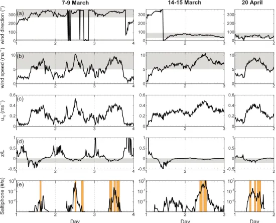
Figure 4. Main characteristics of the 7–9 March, 14–15 March, and 20 April events (left, middle, and right columns,
respectively): time variations of the (a) mean wind direction, (b) mean wind speed at 3-m height, (c) surface friction velocity, (d) stability, and (e) mean impact number of saltating particles recorded by one of the Saltiphone. The shaded areas delimit the values considered for selecting the 15-min time periods in our analysis. The orange vertical areas in (e) correspond to the sampling periods of the Big Spring Number Eight.
a few tens of centimeters downwind from the anemometer, that could have perturbed the measurement for this specific wind direction. However, no flow distortion was observed in our data set in terms of tilt angle and modified wind direction. This correction improved the continuity at 3-m height of the mean velocity profiles and of the horizontal velocity variance profiles obtained from the sonic anemometers. Importantly, we care-fully checked that this correction has a limited impact on the momentum flux at 3-m height and has overall no consequences on the main results obtained in this study.
Finally, in both EC and LoW approaches, the Monin-Obukhov length L involved in the wind velocity profile (equation (1)) has been simply deduced from⟨w′𝜃′⟩ and ⟨u′w′⟩ obtained from the sonic anemometers (e.g., Dupont & Patton, 2012).
3.4. Wind Events
Among the several strong wind events recorded during the experiment, we selected three main events well established for several hours with constant mean wind direction and with 15-min average wind speed higher than 5 ms−1at 3.0-m height. The main characteristics of these three wind events are presented in Figure 4 and summarized in Table 1. The first event corresponds to three consecutive daytime events that occurred on 7–9 March, and those were characterized by northwesterly winds. The second event started on 14 March around noon, finished at the end of 15 March, with a lower intensity early on 15 March and was characterized by a constant northeasterly wind. The third event occurred on 20 April during daytime and was characterized by northeasterly winds. Hereafter, these three events will be referred to as either the 7–9 March, 14–15 March, and 20 April events or the first, second, and third wind events, respectively.
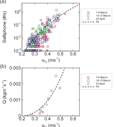
The three wind events were associated with soil erosion as shown by the Saltiphone’s recording in Figure 4e. Both Saltiphone’s recording and saltation fluxes Q show a clear increase of soil erosion with the surface friction velocity u∗0(Figures 5a and 5b). The best fit of the Saltiphone’s recording as a function of u∗0leads to a
Table 1
Main Characteristics of the Selected Wind Events: Surface Friction Velocity Deduced From the Eddy Covariance Approach (u∗0), Wind Direction, Stability (z∕L), and Number of Selected 15-Min Time Periods (Nb 15 Min)
Events u∗0(ms−1) Wind direction (deg) z∕L Nb 15 min
7–9 March 0.33 (±0.07) 322 (±50) −0.07(±0.05) 94
14–15 March 0.32 (±0.07) 60 (±11) −0.02(±0.04) 131
20 April 0.32 (±0.06) 50 (±11) −0.07(±0.05) 53
Note. Between parentheses are indicated the standard deviations. The criteria chosen to select the 15-min time periods
are presented in section 3.4.
threshold friction velocity u∗0taround 0.22 ms−1(Figure 5a). The increase of Q fits well with the third power of u∗0(Figure 5b), in particular the parametrization of Lettau and Lettau (1978): Q = c
√ dp∕D𝜌u2∗0 ( u∗0− u∗0t ) ∕g, where D is a reference grain diameter (= 250μm), dpthe mean grain diameter (= 102μm here), and𝜌 the air density. We obtained a coefficient c near 0.5, which is smaller than the value of 4.2 proposed by Lettau and Lettau (1978). This lower value may be explained by the smaller impact velocity of saltating particles dur-ing our experiment due to their small size. A similar magnitude of saltatdur-ing flux was observed by Zhang et al. (2016) from a wind tunnel experiment with a single mode of soil grain diameter around 100μm. Their coefficient c ranged from 0.27 to 0.86, following their soil configuration.
For all events, we only selected 15-min periods with near-neutral conditions (−0.2 < z∕L < 0.01), signif-icant wind speed (≥5 ms−1 at 3-m height), and wind directions≤20∘ or ≥270∘ for the 7–9 March event and between 30∘ and 90∘ for the 14–15 March and 20 April events (see the shaded areas in Figure 4).
Figure 5. Mean impact number of saltating particles recorded by the Saltiphone (a) and saltation fluxQ(b) against the surface friction velocity (u∗0) obtained for the 7–9 March, 14–15 March, and 20 April events. Saltiphone’s values have been averaged over 15-min periods while saltation fluxes have been averaged over 1 to 4 hours depending on the Big Spring Number Eight collecting time period. The best fit in (a) was obtained for110.4u7.7
∗0, which leads to a threshold friction velocityu∗0tnear 0.22 ms−1below which the Saltiphone did not detect particle impaction. The fitted curve in (b) corresponds to the parameterization of Lettau and Lettau (1978) withc = 0.5(see the text). The mean square error between this parametrization and the observations is±40%, with a coefficient of determinationr2= 0.80.
Periods with mean square deviations between measured and fitted wind velocities higher than 5% were dis-carded. Table 1 gives the number of 15-min periods considered for each wind event considering the above screening criteria.
4. Results
4.1. Wind Dynamics
We found it important to first control the main characteristics of the wind dynamics during the selected events before evaluating the aerodynamic parameters (friction velocity and roughness length) and the von Karman constant.
For the three wind events, the mean wind velocity (⟨u⟩) exhibits a well-defined logarithmic profile along the vertical profile (Figure 6). Sonic and cup anemometers show the same velocity amplitude and variation with height (Figure 6, left column). Both standard deviations of the horizontal wind velocity components (⟨𝜎u⟩, ⟨𝜎v⟩) appear close to each other, the streamwise component being slightly higher for the second event, and both appear almost constant with height (Figure 6, right column). As expected, the standard devia-tion of the vertical wind velocity component (⟨𝜎w⟩) is lower and increases with height. The ratios between the velocity standard deviations and the friction velocity are consistent with known values observed in the turbulent surface layer:⟨𝜎u⟩ ∕ ⟨u∗⟩ ≈ 2.75 and ⟨𝜎w⟩ ∕ ⟨u∗⟩ ≈ 1.25 against 2.50 and 1.25, respectively (Raupach et al., 1996).
The mean local friction velocity⟨u∗⟩, and thus the mean momentum flux (⟨u′w′⟩), appears almost constant with height (Figure 6, middle); it decreases slightly near the surface (1-m height) and remains constant above for the 7–9 March event, while it slightly increases with height above 2 m for the 14–15 March and 20 April events. This increase with height could be related to the limited fetch in the northeast direction, the top of the profile being possibly contaminated by turbulence established with the rougher upwind surface outside the plot. This limited fetch does not seem to occur for the 7–9 March event as the plot is longer in the northwest direction (see Figure 1c). Overall, the average mean square deviations between u∗and the median value of the four anemometer heights (u∗mEC) are below 10% of u∗mEC(about 6%, 8%, and 9% for the first, second, and third events, respectively), which remains quite reasonable.
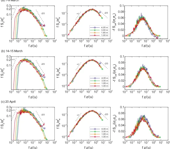
To identify the eddy scales of the main turbulent structures contributing to the velocity variances and to the turbulent transport of momentum (u-w correlation), Figure 7 presents for all events the ensemble-averaged spectra of the streamwise and vertical velocity components (Suand Sw) and u-w cospectrum (Suw) obtained at four heights above the surface from the four sonic anemometers. The frequency f has been normalized using the measurement height z and the mean wind speed at the same height⟨u(z)⟩. The normalized wind spectra at the four heights match nicely together. They display the familiar shape of atmospheric surface layer spec-tra with a well-defined −2∕3 power law in the inertial subrange and +1 power law in the energy-containing range for the w spectra. The peak positions of the u and w spectra are distant from each other, 0.008 and 0.32, respectively. The w peak position is close to the referenced value of 0.28 usually observed in the surface layer (Kaimal et al., 1972), while the u spectrum peaks at a lower frequency than the value of 0.045 reported in Kaimal et al. (1972). This lower frequency of the main u fluctuations observed here could be explained by the lower roughness of our bare surface compared to the crop surface covered with wheat stubble of Kaimal et al., 1972’s experiment. This distance between u and w spectrum peaks reflects the longitudinal elongated shape of turbulent structures near the surface. Our lower surface roughness length (<10−3m) may have accen-tuated this elongated shape of turbulent structures. The scale of the main turbulent structures transporting momentum is intermediate between the scales of the eddies contributing the most efficiently to longitudinal and vertical wind fluctuations. The peak of the u-w cospectrum is around 0.03, which is near the value of 0.07 reported in Kaimal et al. (1972). These results confirm that the length of our averaging procedure (15 min) and frequency of measurements (even close to the surface, at 1-m height) include all the main turbulent structures contributing to the wind turbulence and momentum transport.
To summarize, the wind dynamics observed during our experiment are consistent with usual observations in the surface layer in terms of mean profiles and main turbulent structures. The slight increase of the momen-tum flux at the top of the profile during the 14–15 March and 20 April events may indicate a shorter fetch at 4-m height for northeasterly winds although the mean velocity profile exhibits a perfect logarithmic form along the whole vertical profile.
Figure 6. Mean vertical profiles of the wind velocity deduced from cup and sonic anemometers (left column), local
friction velocity (middle column), and standard deviations of the longitudinal (blue line with squares), lateral (green line with triangles), and vertical (red line with circles) velocity components (right column), obtained for the 7–9 March (a), 14–15 March (b), and 20 April (c) events. The error bars show the standard deviation of each variable. The symbol⟨⟩ denotes the average over all selected 15-min time periods of each wind events.
Figure 7. Ensemble-averaged normalized spectra of the longitudinal and vertical wind velocity components (left and
middle columns) andu-wcospectra (right column) obtained at four levels above the surface, for the 7–9 March (a), 14–15 March (b), and 20 April (c) events. The frequencyfis normalized by the mean wind speed⟨u⟩and the heightz.
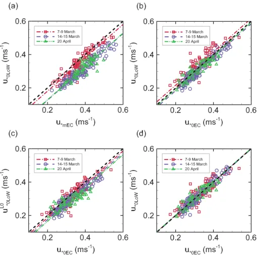
4.2. Friction Velocity
The median value of the friction velocities u∗mECobtained by eddy covariance from the 4 sonic anemometers is compared in a scatter plot with the friction velocity u∗0LoWobtained from the LoW approach (Figure 8a). The friction velocities deduced from the EC approach appear larger than the ones deduced from the LoW approach, especially for the second and third events: +0.02 ms−1for the 7–9 March event and +0.07 ms−1for the 14–15 March and 20 April events.
The agreement between both approaches is improved when substituting for u∗mECwith the extrapolated value at the surface of the friction velocity obtained by eddy covariance u∗0EC(equation (3) and Figure 8b). Only a small bias is perceptible between u∗0LoWand u∗0EC: u∗0ECis slightly underestimated during the first wind event (−0.02 ms−1) and overestimated during the second (+0.02 ms−1) and third (+0.01 ms−1) events. The mean square errors between u∗0ECand u∗0LoWare only ±0.04, ±0.02, and ±0.03 ms−1for the first, second, and third events, respectively. Most of the variability between u∗0LoWand u∗0ECis random and could be attributed to measurement uncertainty, ±6% for u∗0LoWand ±14% for u∗0EC(see Appendix A).
Neglecting the stability correction in the evaluation of u∗0LoW, that is, Ψm= 0 in equation (2), leads to different biases between u∗0LoWand u∗0EC, but the mean square errors remain similar (Figure 8c). The biases become +0.01, +0.02, and +0.03 ms−1for the first, second, and third events, which indicates an average modifica-tion of u∗0LoWgoing up to 10% for the first event. This highlights the sensitivity of u∗0LoWto Ψmand thus the importance of accounting for stability correction in the LoW, even in near-neutral conditions.
A small difference in height of the anemometer profile significantly changes u∗0LoWthrough the slope A of the velocity profile against[log(z) − Ψm
(z L
)]
, while the evaluation of u∗0ECis less affected. For a demonstration, the mean bias between u∗0LoWand u∗0ECin Figure 8b was removed by subtracting 3 cm from all anemometer heights for the 7–9 March event and by adding 3 cm and 2 cm to all anemometer heights for the 14–15 March
Figure 8. Comparison of the friction velocities obtained from the eddy covariance (EC) and law of the wall (LoW)
approaches for 7–9 March, 14–15 March, and 20 April events. (a) The friction velocity from the EC approach corresponds to the median value of local friction velocity obtained from the four sonic anemometers (u∗mEC). (b) The friction velocity from the EC approach corresponds to the extrapolated value at the surface of the local friction velocities obtained from the four sonic anemometers (u∗0EC). (c) The friction velocity from the LoW approach has been deduced by neglecting the stability functionΨmin equation (2) (uL0∗0LoW) and the friction velocity from the EC approach corresponds tou∗0EC. (d) Same as (b) but by removing (adding) 3 cm (3 and 2 cm) to all anemometer heights for the 7–9 March event (14–15 March and 20 April events, respectively). The black dashed line indicates the 1:1 relationship; the dash-dotted red line represents the linear regression of the 7–9 March event dots; the long-dashed blue line represents the linear regression of the 14–15 March event dots; the dash-dotted-dotted green line represents the linear regression of the 20 April event dots.
and 20 April events, respectively. With this correction on the ground level (zsurf), the agreement between u∗0LoWand u∗0ECis improved (Figure 8d). A difference in zsurfbetween the three events could be explained by the modification of the surface during soil erosion or by a difference in horizon following the wind direction, although our site was relatively flat. Both reasons add to uncertainties in our measurements of anemometer heights at the beginning of the experiment. However, a difference of 6 cm in ground level between north-west and northeast directions appears quite large and thus may not explain the whole bias observed between
u∗0LoWand u∗0EC. Furthermore, applying such a correction on zsurfwould mean to consider as true the von Karman constant of 0.40 chosen in the LoW approach. This is why we preferred to not consider hereafter any correction on zsurf.
In conclusion, the mean biases observed between u∗0LoWand u∗0ECin Figure 8b remain small for all wind events. These biases could be explained by different combined effects such as (1) the value of the von Karman constant that was fixed at 0.40 in the LoW approach, (2) the stability function Ψm, or (3) the definition of the ground level (zsurf= 0) used to define the heights of the anemometers. It is difficult to estimate which part of the bias between u∗0LoWand u∗0ECis due to one of these possible reasons.
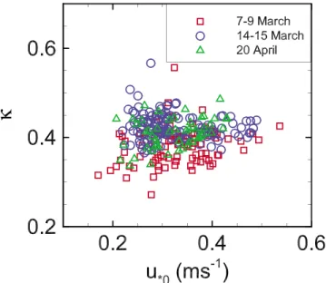
Figure 9. The von Karman constant (𝜅) against the surface friction velocity (u∗0) obtained for the 7–9 March, 14–15 March, and 20 April events.
4.3. Von Karman Constant
Including all wind events, we obtained a von Karman constant𝜅 close to 0.407, with a 68.3% confidence interval on this mean value of ±0.002 (Figure 9). This value is close to the usual values considered in the lit-erature (0.40–0.41) and thus comforts us in choosing𝜅 = 0.40 for estimating u∗LoW. The random variability in𝜅 depicted in Figure 9 is characterized by a standard deviation of ±0.039 (±10%), which is similar to the variability usually observed in studies quantifying𝜅 (e.g., Andreas et al., 2006, 1996; Andreas et al., 2006). This variability is mainly explained by uncertainties of measurements. Our uncertainty analysis led to an expected error on𝜅 of around ±15% (see Appendix A).
However, a significant difference in𝜅 mean value exists between wind events. Our measurements lead to
𝜅 = 0.382 ± 0.004, 0.423 ± 0.003, and 0.409 ± 0.005 for the first, second, and third events, respectively. As for
the friction velocity, we suspect that a part of this difference between events could come from variations of
zsurfor the stability function.
Importantly,𝜅 exhibits no dependence on the surface friction velocity for each event (Figure 9), and therefore no dependence on wind erosion intensity since saltation increases with surface friction velocity (Figure 5).
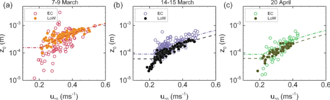
4.4. Roughness Length
The roughness lengths obtained from the EC and LoW approaches (z0ECand z0LoW) show on average a similar behavior with u∗0(Figure 10). They both increase with u∗0, especially for z0LoW, which is consistent with the gen-eral picture of enhancement of the apparent surface roughness due to the presence of saltating particles that absorb momentum from the flow. Without wind erosion, z0ECand z0LoWshould only represent the roughness length of the surface and remain constant for u∗0lower than the threshold value u∗0t= 0.22 ms−1(horizontal lines in Figure 10). However, it is difficult to find sufficient 15-min periods with u∗0lower than u∗0tto confirm this tendency as for such low wind condition, the thermal stratification deviates from the near-neutral con-ditions. As in several previous observations (Farrell, 1999; Gillette et al., 1998; Owen, 1964; Rasmussen et al., 1985), z0seems to scale with the square of u∗0, in the presence of wind erosion (u∗0 ≥ u∗0t), z0 ≈ Ccu2
∗0∕g, where g is the gravitational acceleration. For the first event, both LoW and EC approaches lead to Cc = 0.03 although z0ECpoints appear quite scattered, while for the second and third events the LoW approach leads to Cc= 0.01 and the EC approach to Cc= 0.02. Overall, these Ccvalues are close to the value of 0.02 obtained by Owen (1964).
The difference in z0between the first and the two others wind events, for the same values of u∗0, is certainly explained by the difference in wind sector, and thus a difference in surface influencing the anemometer mea-surements. The bias between z0ECand z0LoW, especially for the last two events, may have the same origin
Figure 10. Variation of the surface roughness length (z0) as a function of the surface friction velocity (u∗0) deduced from the eddy covariance (EC) and law of the wall (LoW) approaches, and obtained for the 7–9 March (a), 14–15 March (b), and 20 April (c) events. The lines represent the best fit ofz0toCcu2∗0∕g. In (a),Cc = 0.03for both EC and LoW
approaches (dash-dotted and dashed lines, respectively). In (b) and (c),Cc = 0.02and 0.01 for EC and LoW approaches (dash-dotted and dashed lines), respectively. For friction velocities lower than the threshold value of 0.22 ms−1deduced from Figure 5, the average behavior of roughness lengths has been assumed constant.
as the bias between u∗0ECand u∗0LoW: the fixed value of the von Karman constant in the EC approach (𝜅 = 0.40) while z0LoWis estimated independently of𝜅, the definition of zsurf, and/or the parameterization of the stability function Ψm.
The random variability around the mean z0values depicted in Figure 10 appears larger for z0ECthan for z0LoW. The mean square errors between z0and Ccu2∗0∕g obtained with the EC are ±94%, ±42%, and ±45% for the first, second, and third events, against ±23%, ±19%, and ±18%, respectively, with the LoW approach. Most of this variability on the roughness length values reported in Figure 10 is explained by uncertainties of the measurements. Our uncertainty analysis shows that the 68.3% confidence interval is wider for z0ECthan z0LoW: 0.6z0LoW ≤ z0LoW ≤ 1.6z0LoWand 0.3z0EC ≤ z0EC ≤ 2.6z0EC(Appendix A). This larger uncertainty of z0ECis explained by the larger uncertainty of u∗0ECthan of u∗0LoW. Importantly, our uncertainty analysis shows that the LoW approach is more appropriate to estimate the surface roughness length than the EC approach since
z0LoWdepends only on first-order moment and𝜅 does not have to be predefined.
5. Discussion and Conclusion
Two friction velocities have been deduced from the EC approach, the mean friction velocity within the sur-face layer (u∗mEC) and the extrapolated friction velocity at the surface (u∗0EC). Both were obtained from the four sonic anemometers located between 1.0- and 4.1-m height. Compared to the friction velocity obtained from the LoW approach (u∗0LoW), u∗mECwas 20% larger, while u∗0ECwas in good agreement with u∗0LoW, regardless of the wind intensity. The mean square error between u∗0LoWand u∗0ECwas only ±0.04 ms−1, and no significant bias was observed. Hence, extrapolating the local friction velocities obtained by EC to the surface instead of averaging them seems to solve most of the discrepancy in u∗between LoW and EC approaches. This result was obtained after carefully checking the main characteristics of the wind dynamics and turbulent structures by comparison with expected behavior in the surface layer. This result confirms that the friction velocity appear-ing in the logarithmic form of the velocity profile is representative of the shear stress at the surface, and not of the average shear stress in the surface layer.
Although u∗should be constant with height in an ideal surface layer, in reality a perfect constant flux layer is rarely observed. In our measurements, the average mean square deviations between local u∗and u∗mECwere lower than 10%. As discussed in Andreas et al. (2006), the variability of u∗with height could be explained by the imperfect stationarity of the surface layer compared to flows in a wind tunnel. This, however, should not lead to a specific trend of the mean u∗with height as observed in some of our wind events. We suspect that the slight increase with height of the mean u∗observed in particular for northeasterly winds was a conse-quence of a limited fetch, the upper profile being possibly contaminated by turbulence established with the rougher upwind surface outside the plot. Despite this imperfect constant flux layer, the mean velocity pro-file was always logarithmic (mean square deviations<5%). Observing a logarithmic velocity profile does not necessarily mean a constant flux layer.
Our measurements suggest an average value of the von Karman constant𝜅 of 0.407 ± 0.002. This mean value is remarkably close to the value of 0.40–0.41 usually taken in the literature. Importantly,𝜅 was found inde-pendent of the wind intensity (Figure 9) and thus, indeinde-pendent of the soil erosion intensity since the saltation flux was clearly increasing with wind intensity (Figure 5). Although individual wind events exhibits small dif-ferences in average values of𝜅: 𝜅 = 0.382 ± 0.004, 0.423 ± 0.003, and 0.409 ± 0.005 for the 7–9 March, 14–15 March, and 20 April events, respectively, these differences appear uncorrelated with the saltation intensity. We do not have a clear explanation for these small differences in𝜅 between events. The intraday variability of
𝜅 during the first and second events does not exhibit any particular tendency or difference (result not shown).
The high uncertainty of individual 15-min values of𝜅 (±15%) makes it harder to explain small differences on
𝜅 mean values between events. We suspect that a part of these differences could be related to uncertainty
associated with the stability correction or the variability in ground level (zsurf) between erosion events since the first wind event did not have the same wind directions as the two others and since the last wind event was more than 1 month later than the first two.
The observed independence of𝜅 to wind erosion intensity contradicts the reduction of 𝜅 with saltation observed by Li et al. (2010). They explained their𝜅 reduction with the decrease of the turbulent mixing effi-ciency in presence of sediments in the flow although their measurements were above the saltation layer. Compared to Li et al. (2010), our saltation fluxes were lower by a factor of 10, while our friction velocities nor-malized by the threshold friction velocity (u∗0∕u∗0t) were higher, ranging from 0.8 to 2.5 against 0.9 to 1.8 in Li et al. (2010). Two main reasons could explain this apparent contradictory behavior. First, the lower median grain diameter of our soil, 102 μm against 300 μm in Li et al., 2010, decreases u∗0tand also the particle impact velocity, which consequently reduced the saltation flux. A similar reduction of saltation flux with particle size was observed by Zhang et al. (2016) from a wind tunnel experiment. Second, our sampling periods for col-lecting sediments with the BSNE were much longer than in Li et al. (2010) (1 to 4 hr compared to 2 to 5 min). Hence, our sampling periods may have included periods of low saltation due to both saltation intermittency and wind variability. Overall, the nonsensitivity of𝜅 value to wind erosion in our experiment may suggest that the apparent increase of𝜅 suggested by Li et al. (2010) could simply be due to a nonconstant flux layer. Indeed, Li et al., 2010’s experiment was limited by only one eddy covariance level at 1-m height, making it impossible to verify the presence of a constant flux layer. This led them to assume equality between the fric-tion velocity obtained at this height and the surface fricfric-tion velocity and thus to assume that the difference in u∗between LoW and EC approaches was due to a modification of𝜅. Our findings on the nonsensitivity of
𝜅 to wind erosion are also confirmed by the conclusion of Lee and Baas (2016) who observed no dependence
on wind erosion of their difference in u∗between LoW and EC approaches, meaning that the𝜅 value was independent of the wind erosion intensity.
Overall, several reasons could explain the difference in u∗between EC and LoW approaches observed in pre-vious field experiments (Lee & Baas, 2016; Li et al., 2010). Some of them have been already discussed by these authors. We would like here to highlight four of them. First, the hypothesis of equality between u∗at the surface and above the surface could be the main reason for the observed differences, in particular because previous studies never observed a constant flux layer or were unable to verify its existence due to an unique sonic anemometer. Second, neglecting the stability correction function Ψmin the logarithmic wind velocity profile (equation (1)) can significantly modify the estimated value of u∗0LoW, even in near-neutral conditions. In our experiment, although Ψmrepresented only 3% of log
(
z∕z0 )
in the wind velocity profile (equation (1)), neglecting Ψmcould have led to a difference in u∗0LoW of up to 10%. Third, an accurate definition of the ground level (zsurf) used to define the anemometer heights appears crucial for estimating u∗0LoW. Our analysis highlighted that a difference of a couple of centimeters can lead to a few 0.01 ms−1bias between u
∗0ECand u∗0LoW(see section 4.2). Fourth, the sampling frequency of sonic anemometers in Li et al. (2010) and Lee and Baas (2016), 32 and 50 Hz, respectively, may have been too low for measurements below 1-m height, down to 0.115-m height in Lee and Baas (2016). These small sampling frequencies may have missed a portion of the high-frequency fluctuations of w and thus underestimated the friction velocity by not accounting for the momentum transport by the smallest eddies near the surface. Unfortunately, Li et al. (2010) and Lee and Baas (2016) did not present any spectra of their vertical wind velocity component or cospectra of their momentum flux to verify the adequacy of their anemometer sampling frequency. Additionally, the 2- to 5-min averaging time chosen by Li et al. (2010) to derive the friction velocity from their sonic anemometer may also have been too low, missing the contribution from large eddies to the momentum transport. Our analysis showed that 15 min was the lowest limit for an averaging time at 1-m height in order to account for all eddies contributing
to the momentum flux (Figure 2), and a sampling frequency of 60 Hz at 1-m height was a minimum to obtain the inertial range of the w spectrum (Figure 7).
To conclude, surfaces subject to aeolian soil erosion in semiarid regions often do not respond to the ideal characteristics of application of the LoW, in particular regarding the surface flatness and extent. Even in opti-mal conditions, accurately estimating a friction velocity above these surfaces is challenging. This needs to be remembered when using the friction velocity to scale erosion fluxes or to estimate dust flux from the flux-gradient relationship. The present study leads to the following recommendations:
1. The surface friction velocity has to be deduced either from a vertical profile of several eddy covariance measurements or from the LoW with a good resolution of the wind starting from the upper saltation layer. Estimating the surface friction velocity from only one level of eddy covariance measurement is inaccurate, even for an apparently homogeneous surface, and thus less accurate for inhomogeneous sites.
2. Aerodynamic parameters (u∗and z0) would be better deduced independently of𝜅 because of the variability of𝜅 values at the scale of the erosion event. This means to deduce z0from the regression of the logarithmic wind speed profile and u∗from the eddy covariance approach.
3. Neglecting the stability correction in the LoW could lead to significant differences in the estimated values of the aerodynamic parameters, even in near-neutral conditions.
4. Aerodynamic parameters are sensitive to the ground level definition, especially when deduced from the LoW approach. Consequently, the ground level surrounding the measurement mast has to be care-fully assessed in all wind directions and reassessed during the field experiment to account for surface modification due to soil erosion.
5. When deducing a friction velocity from the EC approach, the spectra of the wind velocity components and momentum cospectrum have to be checked in order to verify that the choice of the averaging time and sampling frequency of the sonic anemometers is adequate to account for the main eddies responsible for the momentum flux.
6. Since the friction velocity deduced from the LoW approach is representative of the surface wind shear stress,
u∗0LoWappears appropriate for scaling saltation fluxes or for defining the threshold friction velocity above which erosion starts. However, as a consequence of the imperfect constant flux layer, u∗0LoWmay not be appropriate for estimating dust fluxes at a few meters height (z) above the surface from the flux-gradient relationship as u∗0LoWmay not accurately represent the velocity scale of the turbulent diffusivity at this level. A local evaluation of the friction velocity from the eddy covariance approach may be more accurate in that case.
Appendix A: Uncertainty Analysis
The uncertainties on friction velocities (u∗0LoW, u∗0EC), roughness lengths (z0LoW, z0EC), and von Karman con-stant (𝜅) were evaluated by means of Monte Carlo simulations. The approach used to estimate these variables was reproduced in multiple simulations (105) from typical wind event values of the mean wind speeds (⟨u⟩), momentum fluxes (⟨u′w′⟩), and stability function (Ψ
m) where random variabilities were added to their mean values in order to simulate the propagation of prescribed individual uncertainties to the final results. Monte Carlo simulation method was preferred from the conventional uncertainty analysis method as it allows to quantify more accurately the propagation of uncertainties in complex nonlinear systems (Herrador & González, 2004; Papadopoulos & Yeung, 2001).
A1. Sources of Uncertainty
We identified four sources of uncertainty: (1) the mean wind speed deduced from cup anemometers and used to fit the LoW, (2) the momentum flux estimated by eddy covariance from the sonic anemometers, (3) the origin of the ground surface defining the heights of the cup and sonic anemometers, and (4) the stability function used in the LoW. All four quantities (𝛼) were characterized by their own uncertainty Δ𝛼assuming a normal distribution of their values. Their uncertainties Δ𝛼were defined as the percentage of their standard deviation𝜎⟨𝛼⟩of the mean value⟨𝛼⟩ relative to ⟨𝛼⟩: Δ𝛼=𝜎⟨𝛼⟩∕⟨𝛼⟩. This means that there is a 68.3% probability of having a value between⟨𝛼⟩ − Δ𝛼⟨𝛼⟩ and ⟨𝛼⟩ + Δ𝛼⟨𝛼⟩.
The main source of uncertainty for⟨u⟩ and ⟨u′w′⟩ is related to sampling error due to the limited number of independent samples contributing to the mean during the chosen averaging time T (15 min) (Businger, 1986). Increasing the averaging time would reduce the uncertainty, but the condition of stationarity of the
Table A1
Summary of the Considered Sources of Uncertainties and the Resulting Propagated Uncertainties Obtained From the Monte Carlo Simulations
Variables Denomination Uncertainty
Sources of uncertainty
zsurf Ground surface origin ±1cm
⟨u⟩ Mean wind speed obtained from cup anemometers ±2%
u∗ Local friction velocity deduced from sonic anemometers ±10%
Ψm Stability function ±2%
Resulting propagated uncertainty
u∗0LoW Surface friction velocity obtained from the LoW approach ±6%
u∗0EC Surface friction velocity obtained from the EC approach ±14%
z0LoW Surface roughness length obtained from the LoW approach 0.6z0LoW≤ z0LoW≤ 1.6z0LoW z0EC Surface roughness length obtained from the EC approach 0.3z0EC≤ z0EC≤ 2.6z0EC
𝜅 von Karman constant ±15%
Note. The uncertainties correspond here to the 68.3% confidence interval over the 15-min average values. LoW = law of
the wall; EC = eddy covariance.
sampling period may be less verified (Finkelstein & Sims, 2001). The error level of a turbulent quantity𝛼 can be expressed as Δ𝛼=(𝜎𝛼∕⟨𝛼⟩) √2𝜏𝛼∕T, where𝜎𝛼and⟨𝛼⟩ are the standard deviation and the mean of 𝛼, and
𝜏𝛼is the integral time scale of𝛼 (scale of independent measure) (Kaimal & Finnigan, 1994). The integral time scale can be deduced either from the spectrum peak or from the autocorrelation function.
For⟨u⟩, the ratio 𝜎u∕⟨u⟩ is typically around 0.14 and 𝜏uis about 5 s during our wind events. This leads to a ±2% uncertainty on⟨u⟩. For ⟨u′w′⟩, 𝜎
u′w′∕⟨u′w′⟩ is around 4 and 𝜏u′w′is about 1 s, leading to a ±20% uncertainty,
and thus a ±10% uncertainty on the local friction velocity u∗. This large uncertainty on the momentum flux is typical of eddy covariance fluxes (see, e.g., Kaimal & Finnigan, 1994; Rannik et al., 2016). For the same averaging period, higher moments have lower accuracy than lower moments due to increasing variability compared to mean value (𝜎𝛼∕⟨𝛼⟩) with the order of the moment (Kaimal & Finnigan, 1994).
We estimated the uncertainty on the origin of the ground surface as ±1 cm. This value includes error in measurements and variability of the surface during the experiment as the surface changed with soil erosion. Since all our selected measurement periods were in near-neutral conditions, we applied a ±2% uncertainty on Ψmas proposed by Andreas et al. (2006) based on the variability of the multiplicative constant in Ψmreported in the literature.
A2. Friction Velocity Uncertainty
Error on u∗0LoWis related to the uncertainty of the slope A of the regression of⟨u⟩ on [
log(z) − Ψm (z
L )] (see equation (2)). In our Monte Carlo trials, the mean wind speed profile was characterized by a mean fric-tion velocity of 0.32 ms−1, a roughness length of 5 × 10⁻⁴m, a Monin-Obukhov length of −43 m, and with the anemometer heights given in section 3. The simulations led to a range of u∗LoWvalues normally distributed from which we identified an uncertainty of ±6% (68.3% confidence interval).
Error on u∗ECdepends on the uncertainty of the intercept of the regression of u∗on z (see equation (3)). The mean profile of u∗was chosen as 0.0164z + 0.3431, which fits the mean profile of Figure 6a. The simulations led to u∗ECwith also a normal distribution from which we identified an uncertainty of ±14%.
Note that the uncertainty of u∗ECis more important than that of u∗0LoW. This is explained by the evaluation of u∗LoWfrom a first-order moment (⟨u⟩) while u∗ECis deduced from a second-order moment (⟨u′w′⟩), the former moment having higher accuracy than the later one for the same averaging period, as explained in section A1.
A3. Roughness Length Uncertainty
Error on z0LoW depends on the uncertainty of the slope A and intercept B of the regression of ⟨u⟩ on [ log(z) − Ψm ( z L )]