HAL Id: hal-00340115
https://hal.archives-ouvertes.fr/hal-00340115
Preprint submitted on 19 Nov 2008
HAL is a multi-disciplinary open access
archive for the deposit and dissemination of
sci-entific research documents, whether they are
pub-lished or not. The documents may come from
teaching and research institutions in France or
abroad, or from public or private research centers.
L’archive ouverte pluridisciplinaire HAL, est
destinée au dépôt et à la diffusion de documents
scientifiques de niveau recherche, publiés ou non,
émanant des établissements d’enseignement et de
recherche français ou étrangers, des laboratoires
publics ou privés.
On the frequency of N2H+ and N2D+
Laurent Pagani, Fabien Daniel, Marie-Lise Dubernet
To cite this version:
Laurent Pagani, Fabien Daniel, Marie-Lise Dubernet. On the frequency of N2H+ and N2D+. 2008.
�hal-00340115�
Astronomy & Astrophysicsmanuscript no. freq˙n2hp.hyper7668 c ESO 2008 November 19, 2008
On the frequency of N
2
H
+
and N
2
D
+⋆
(Research Note)
L. Pagani
1, F. Daniel
1,2, and M.L. Dubernet
11 LERMA & UMR8112 du CNRS, Observatoire de Paris, 61, Av. de l’Observatoire, 75014 Paris, France
e-mail: laurent.pagani@obspm.fr, marie-lise.dubernet@obspm.fr
2 Department of Molecular and Infrared Astrophysics ( DAMIR), Consejo Superior de Investigaciones Cient´icas (CSIC ), C/ Serrano
121, 28006 Madrid, Spain
e-mail: daniel@damir.iem.csic.es received : 11/7/2008; accepted : 10/11/2008
ABSTRACT
Context.Dynamical studies of prestellar cores search for small velocity differences between different tracers. The highest radiation frequency precision is therefore required for each of these species.
Aims.We want to adjust the frequency of the first three rotational transitions of N2H+and N2D+and extrapolate to the next three
transitions.
Methods.N2H+and N2D+are compared to NH3the frequency of which is more accurately known and which has the advantage to be
spatially coexistent with N2H+and N2D+in dark cloud cores. With lines among the narrowests, and N2H+and NH3emitting region
among the largests, L183 is a good candidate to compare these species.
Results.A correction of ∼10 kHz for the N2H+(J:1–0) transition has been found (∼ 0.03km s−1) and similar corrections, from a
few m s−1up to ∼0.05 km s−1are reported for the other transitions (N
2H+(J:3–2) and N2D+(J:1–0), (J:2–1), and (J:3–2)) compared to
previous astronomical determinations. Einstein spontaneous decay coefficients (Aul) are included.
Key words.Molecular data – ISM : kinematics and dynamics – ISM : lines and bands – Radio lines : ISM
1. Introduction
In the quest for star forming cores, kinematic studies play a cru-cial role, trying to unveil slowly contracting cores or fast col-lapsing ones, depending upon which theory we rely upon or at what moment along the evolutionary track the prestellar core is standing. As already discussed by Lee et al. (1999), the accurate knowledge of every species line frequency is of the uttermost im-portance to track small systematic velocity gradients in molec-ular clouds. Therefore, because these velocity shifts can be as small as a few tens of m s−1, millimeter line transitions should be
known with a precision of at least 10−7 and ideally 10−8. Some
species are easily measured in the laboratory, especially stable species like CO, NH3, etc,. Others are unstable and more
diffi-cult to measure (such as OH, H2D+,...). One possibility in the
latter case, is to compare the transitions of the species of inter-est with the transitions of another well-known species in dark cloud cores where the lines are narrow enough to be accurately measured. However, the obvious difficulty is to be sure that the two species share the same volume of the cloud and undergo the same macroscopic velocity shifts. Even though, the line opaci-ties might be a problem if too different in presence of a velocity gradient : the two coexistent species might then emphasize dif-ferent parts of the cloud, depending on the depth for which their
Send offprint requests to: L.Pagani
⋆ Based on observations made with the IRAM 30-m and the GBT
100-m. IRAM is supported by INSU/CNRS (France), MPG (Germany), and IGN (Spain). GBT is run by the National Radio Astronomy Observatory which is a facility of the National Science Foundation op-erated under cooperative agreement by Associated Universities, Inc.
respective opacity reaches 1. A problem of opacity was indeed met in the comparison of CS with CCS made by Kuiper et al. (1996) in their attempt to measure the frequency of the CS lines as discussed in Pagani et al. (2001).
Caselli et al. (1995) performed such a measurement for N2H+, comparing N2H+(J:1–0) line emission to the C3H2(JKK′: 212–101) line emission in L1512, confirming a sizeable
differ-ence between laboratory measurement and astronomical obser-vations. Dore et al. (2004) expanding on a previous work by Gerin et al. (2001) also calculated and observed the N2D+(J:1–
0) transition in L183, and extrapolated to the higher N2D+
tran-sitions, (giving slightly different values compared to Gerin et al. 2001, for the J:2–1 and J:3–2 transitions). They aligned their N2D+(J:1–0) observation onto their N2H+(J:1–0) towards the
same source with the same telescope. The N2H+rotational
con-stant was itself redetermined from a new evaluation of the N2H+
(J:1–0) frequency from a comparison with C18O (J:1–0) in the
L1512 cloud (see Dore et al. 2004, for more details). This new value gave an offset of -4.2 kHz from their previous determina-tion.
While the direct comparison of the N2D+and N2H+lines is
presently the best option to choose because N2H+forcibly exists
where N2D+exists, the hypothesis that C3H2is also present in
the same volume as N2H+is more questionable because of
dif-ferential depletion problems. Dore et al. (2004) also note that us-ing C18O has the problem of tracing different regions but hoped
for a null velocity shift between the two tracers. We think that a better possibility exists to measure accurately the frequency of N2H+, namely by taking NH3as the frequency reference. NH3
2 L. Pagani et al.: On the frequency of N2H+and N2D+(RN)
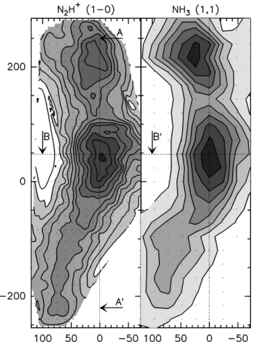
Fig. 1. N2H+(J:1–0) (left) and NH3 (1,1) (right) integrated
in-tensity maps. The dotted lines AA′and BB′indicate the profiles along which the velocity gradients are traced in Figs. 2 & 3. Reference position : α2000= 15h54m08.5sδ2000= -2◦52′48′′
cores (e.g. Tafalla et al. 2002, 2004), having a common chemi-cal origin and showing similar extents in most cores.
In this Note, we present a detailed comparison of NH3with
N2H+and N2D+in L183, checking that the measurable velocity
shifts across the core are the same for all three species to con-vince ourselves of their coexistence and the absence of opacity effect on the velocity peak position. Schmid–Burgk et al. (2004) developed a similar strategy in their study of H13CO+and13CO hyperfine structure (hereafter HFS) towards another dark cloud, L1512, with similar very narrow linewidths. With these compar-isons in hand, we give all corrections for the 5 most currently ob-served transitions together with their Einstein spontaneous decay coefficients (Aul), determine the best fitting rotational constants and compute the expected frequencies for the next 3 rotational transitions (J:4–3, 5–4, 6–5).
2. Observations
The whole elongated dense core of L183 (reference position : α2000 = 15h54m08.5s δ2000 = -2◦52′48′′) has now been fully
mapped wih the IRAM 30-m telescope in a series of observa-tions spanning several years from November 2003 to July 2007. The N2H+and N2D+(J:1–0) lines have been fully mapped while
the N2H+ (J:3–2), N2D+ (J:2–1) and (J:3–2) lines have been
mapped mostly towards the main core and its elongated ridge and partly towards the peak of the northern core (see Pagani et al. 2004, 2005). All observations have been performed in frequency–switch mode. For the (J:1–0) lines, the frequency
sampling is 10 kHz, 10 or 20 kHz for the (J:2–1) and 40 kHz for the (J:3–2) lines, providing comparable velocity resolution for all lines in the range 30–50 m s−1. Spatial resolution ranges from
33′′at 77 GHz to 9′′at 279 GHz. For all lines, the spatial sam-pling is 12′′for the main prestellar core and 15′′for the southern extension and for the northern prestellar core. We use Caselli et al. (1995) and Dore et al. (2004) frequencies for N2H+and N2D+
transitions, respectively.
We performed observations of NH3(1,1) and (2,2) inversion
lines towards the whole core at the new Green Bank 100-m telescope (GBT) in November 2006 and March 2007 with velocity sampling of 20 m s−1 and a typical T
sys of 50 K, in
frequency–switch mode. The angular resolution (∼35′′) is close to that of the 30-m for the low-frequency (J:1–0) N2D+line. The
spatial sampling is 24′′ all over the source. We use the accu-rate measurement of Kukolich (1967) for NH3 (1,1), namely ν = 23 694 495 487 (±48) Hz which is an average estimated from the whole HFS (see also Hougen 1972, who revisited the NH3 and15NH3 frequencies. The reported accuracy is higher
but the NH3 (1,1) frequency remains basically unchanged,
namely ν = 23 694 495 481 ± 22 Hz). For this frequency, the two strongest hyperfine components have the following frequency offsets :
∆ν(F1F : 2,5/2→2,5/2) = 10 463 Hz ∆ν(F1F : 2,3/2→2,3/2) = -15 196 Hz
Samples of these spectra (N2H+, N2D+ and NH3) are
dis-played in Pagani et al. (2007).
3. Spatial coexistence of ammonia and diazenylium
Though depletion of molecules was predicted in the 70’s, it was only a few years after the publication of the Caselli et al. (1995) paper on the frequency of N2H+that depletion was actually
dis-covered and traced (e.g. Willacy et al. 1998). Therefore the hy-pothesis made by Caselli et al. (1995) that C3H2 and N2H+are
spatially coexistent is probably refutable as it is clear now that such heavy Carbon carrier should be depleted in the same re-gion as CO which is the rere-gion where N2H+appears. Indeed,
the detection of N2D+ in L1512 as a large fraction of N2H+
(Roberts & Millar 2007) is a clear sign of heavy depletion of other molecules. Therefore the velocity coincidence between these two species is questionable.
Ammonia and diazenylium have the same chemical origin, starting from N2 and are well-known to be coexistent as
dis-cussed by e.g. Tafalla et al. (2002, 2004). This is in particular true in L183 as can be seen in Fig. 1 (but not for C3H2which has
a much smaller extent, mostly concentrated towards the northern prestellar core as can be seen in Swade 1989). Interestingly, the velocity along the dense filament is constantly changing (Fig. 2), evoking a flow towards the prestellar cores and the cut per-pendicular to the filament (marked BB′ in Fig. 1) is suggest-ing a rotation of the filament around its vertical axis (Fig. 3). NH3 (1,1), N2H+ and N2D+ (J:1–0) all trace exactly the same
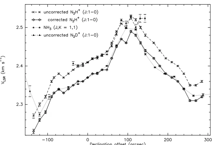
gradients and it seems therefore compulsory that their velocities be identical as there is no obvious possibility that the velocity gradients be exactly parallel but offset from each other, espe-cially in the probable case of the cylinder rotation. With present N2H+(J:1–0) frequency as given by Caselli et al. (1995), there
is indeed a clear offset with respect to the NH3velocity gradient,
close to 40 m s−1 (and to 26 m s−1 compared to the new value
L. Pagani et al.: On the frequency of N2H+and N2D+(RN) 3
Fig. 2. N2H+, N2D+(J:1–0) and NH3(1,1) line of sight velocity along the AA′cut (see Fig. 1). The N2H+data are displayed with
the original frequency (uncorrected) and with a correction of -41 m s−1. The uncorrected N
2D+(J:1–0) points are consistent with
the uncorrected N2H+points despite the different opacities
reinterpreted Caselli et al. (1995) observations along with new laboratory measurements but are therefore plagued by the ve-locity difference between N2H+and C3H2which appears to
ex-ist in view of the present discrepancy between NH3 and N2H+.
Consequently, their best fit (#2 of their Table 2) is to be consid-ered cautiously. Finally, the fact that N2D+velocity centroids are
almost identical with those of N2H+indicates that the different
opacities of the lines are not introducing any measurable bias here (though a very tiny shift is possibly visible in Fig. 3 where the N2D+ displacement is symmetrically slightly less than the
N2H+displacement).
In conclusion, the three species are spatially coexistent and trace the same velocities and one must adjust the frequencies of N2H+and N2D+to that of NH3.
4. Frequency corrections
4.1. N2H+(J:1–0) correction
Frequency was measured using the MINIMIZE function in CLASS1 with the HFS method for all species (for NH3, the
HFS method is similar to the internally built NH3(1,1) method). Because it is easier to deal with velocity offsets in CLASS, es-pecially as we have to compare two species at different fre-quencies, the measurements have all been made in the veloc-ity scale. Velocveloc-ity differences are subsequently converted into frequency offsets using the approximate doppler shift formula
1 http://www.iram.fr/IRAMFR/GILDAS
(ν = ν0(1 − δvc), δv being the velocity offset, c the celerity of
light, ν and ν0the corrected and original frequencies). The HFS
method, in order to fit all the hyperfine components individually requires that we provide their list with their relative velocities and relative weights, these parameters not being adjusted dur-ing the fit. Therefore, we have used the detailed HFS provided by Caselli et al. (1995), Dore et al. (2004) and Kukolich (1967). Since an accurate determination of the hyperfine spectroscopic constants depends only slightly on the adopted rotational con-stants B and D2, we can safely use the previously determined ones. Doing so, our own determination for the relative velocity offsets between the hyperfine components in the J:1–0 line agree with Caselli et al. (1995) with a typical dispersion of 0.7 kHz. Though this is twice as much as the r.m.s. error on our frequency determination of each individual component (σ ∼ 0.3 kHz), we find that using their offsets or ours, introduces a negligible differ-ence of 0.13 kHz in the J:1–0 transition frequency determination, which is comparable to the r.m.s. error of the fit (0.12 kHz). We also did not find an improvement on the r.m.s. error of the fit itself. For the N2H+and N2D+transitions, the strongest
hyper-fine transition was given null velocity offset as it was also the strongest hyperfine transition frequency which was used to tune the receivers. The advantage of a complex and strong HFS is that it lowers the uncertainty on the velocity fit, compared to a sin-gle line estimate (fitting individually the N2H+J:1–0 lines with
2 indeed, it can be noted that the HFS splitting is in first
approxima-tion identical for both N2H+and N2D+despite a large, ∼20% variation
4 L. Pagani et al.: On the frequency of N2H+and N2D+(RN)
Fig. 3. N2H+, N2D+(J:1–0) and NH3(1,1) line of sight velocity
along the BB′cut (see Fig. 1). The N
2H+data are displayed with
the original frequency (uncorrected) and with a correction of -41 m s−1. The uncorrected N
2D+(J:1–0) points are consistent with
the uncorrected N2H+points despite the different opacities
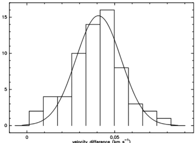
Fig. 4. N2H+(J:1–0) and NH3(1,1) line of sight velocity
differ-ence histogram. The gaussian fit is centered on 40.8 m s−1 with
a dispersion σ = 12.9 m s−1
independent gaussians, gives errors between 0.85 and 1.2 m s−1 instead of 0.38 m s−1 with the global HFS fit for the reference
spectrum).
Though the reference position has been observed often enough to get very high signal-to-noise ratios for most transi-tions, it seems more secure to measure the offset between N2H+
and NH3 on all common positions (every other position in the
central core, a few positions in the rest of the cloud) and measure the average difference. We have identified 65 common positions with sufficient signal-to-noise ratios and we have obtained the dispersion histogram of the velocity difference (Fig. 4). Fitting the histogram with a gaussian, we find a velocity difference of 40.8 m s−1 with a dispersion σ = 12.9 m s−1. This corresponds
to a frequency correction of -13 ± 4 kHz (or -8.8 kHz compared to Dore et al. 2004). For the reference position alone, the differ-ence is also 40.8 m s−1with an error σ = 0.56 m s−1(due to the very high signal to noise ratio obtained for both lines towards that position).
4.2. N2H+(J:3–2) correction
For the N2H+ (J:3–2) transition, only the reference position
has been observed with a reasonably good signal-to-noise
ra-tio (∼10). Therefore, we can only make a direct comparison for this position. The Jet Propulsion Laboratory (JPL) catalogue fre-quency for this line (279 511.701 ± 0.05 MHz) is too vague to be useful for a precise velocity determination. The Cologne Database for Molecular Spectroscopy (CDMS) catalogue gives ν
= 279 511.8577 MHz for the (F1F: 4,5–3,4) strongest hyperfine
component based on various works while Crapsi et al. (2005) give 279 511.863 MHz determined from the new rotational and centrifugal distorsion constants from Dore et al. (2004). These new values are respectively 26 and 31 kHz above our own deter-mination.
4.3. N2D+corrections
For all three transitions of N2D+, we took advantage of the
similar sampling with N2H+ (J:1–0) to have a larger number
of comparison points. We obtained 83, 73 and 51 comparison points with sufficient signal-to-noise ratio between N2H+
(J:1–0) (using Caselli et al. 1995, frequency) and N2D+(J:1–0),
(J:2–1), and (J:3–2) transitions respectively. The gaussian fit to each histogram yielded :
(J:1–0) : -5.1 m s−1(σ = 10.5 m s−1)
(J:2–1) : 12.5 m s−1(σ = 14.4 m s−1)
(J:3–2) : 18.4 m s−1(σ = 8.1 m s−1)
The corresponding correction with respect to NH3(1,1)
is :
(J:1–0) : 35.7 m s−1or -9.2 (± 2.7) kHz
(J:2–1) : 53.3 m s−1or -27 (± 7.4) kHz
(J:3–2) : 59.2 m s−1or -49 (± 6.7) kHz
Direct comparison of the reference position with NH3(1,1)
spectrum yields :
(J:1–0) : 37.7 m s−1(σ = 0.85 m s−1)
(J:2–1) : 47.7 m s−1(σ = 0.92 m s−1)
(J:3–2) : 63.6 m s−1(σ = 4.7 m s−1)
4.4. Rotational constants and Einstein–A coefficients
Except for the N2H+(J:3–2) line which has only one
measure-ment, we have used the averaged comparisons for correcting the frequencies of all these transitions.
We have derived from these new frequencies the rotation (B) and centrifugal distortion (D) constants for N2H+and N2D+,
us-ing the hyperfine constants given by Caselli et al. (1995) and Dore et al. (2004) respectively. The error budget has been es-timated by adding 1 σ to one of the frequency measurements and subtracting 1 σ to the other which we use to determine B and D, e.g. +2.7 kHz to the N2D+ (J:1–0) line and -6.7 kHz
for the N2D+ (J:3–2) line. For the N2H+ (J:3–2) transition, as
we have only one measurement, we have taken the average of the 1σ dispersion for all the other transition measurements as a probable dispersion for that measurement if we had had as many observations. We have found an average velocity dispersion of 11.5 m s−1which corresponds to 10.7 kHz at that frequency. The
new constants are listed in Table 1. As expected from the fact that Amano et al. (2005) make use of the Caselli et al. (1995) frequency determination of N2H+ and the related Dore et al.
dif-L. Pagani et al.: On the frequency of N2H+and N2D+(RN) 5 ferent from ours by an amount directly related to the difference
between C3H2and NH3velocity determinations. The difference
(5.3 kHz for B(N2H+) and 9.2 kHz for B(N2D+)) is significantly
larger than the error estimate (conservatively given to be 2.5 and 1.7 kHz respectively for us and 1.3 and 1.2 kHz for Amano et al. 2005). It would be interesting to repeat Amano et al. (2005) analysis with our new frequency determinations to better secure these values.
Line strengths, from which Einstein–A coefficients are de-fined, are determined from the reduced transition matrix ele-ments of the dipole moment operator:
S (1 → 2) = |Dψ1|| ˆd||ψ2 E
|2 (1)
where |ψ1 >and |ψ2 >are the wave–functions of the two levels
involved in the radiative transition. In the case of hyperfine struc-tures, the wave–functions can be defined according to an expan-sion on Hund’s case (b) wave–functions, the coefficients being determined by diagonalisation of the hyperfine Hamiltonian. In the case of N2H+and N2D+, the mixing of states is low so that
a given hyperfine wave–function can be accuretaley defined as a pure Hund’s case (b) wave–function. Doing so, the line strengths can be expressed in a closed form (Gordy & Cook 1984), and for N2H+, the relevant expressions being given in Daniel et al.
(2006). The Einstein–A coefficients are then given by:
AJF1F→J′F′1F′ = 64π4 3hc3µ 2ν3 JF1F→J′F′1F ′× J [F]sJF1F→J′F′1F′ (2)
(this is the same equation as in Daniel et al. 2006, but corrected for two typos)
The calculated line frequencies and Aul coefficients (the dipole moment – µ = 3.37 D – is taken from Botschwina 1984) are given in Tables 2 to 10 for all rotational transitions from (J:1– 0) to (J:6–5) for both N2H+ and N2D+. The frequency
uncer-tainty is estimated by varying the rotational B and D constants by ±1 σ.
Table 1. Rotation (B) and centrifugal distortion (D) constants for
N2H+and N2D+. Errors in parentheses are given for the last two
digits Species B D MHz MHz N2H+ 46586.8713(25) 0.08796(24) N2D+ 38554.7479(17) 0.06181(15) 5. Conclusions
1. New, more accurate rotational constants and line frequencies are given along with the detailed Einstein spontaneous coef-ficients (Aul) for each of the hyperfine components.
2. The main prestellar core LSR velocity is 2.3670 (±0.0004) km s−1.
Acknowledgements. We thank an anonymous referee for her/his critical reading
which helped to improve the manuscript.
References
Amano, T., Hirao, T., Takano, J. 2005, J. Mol. Spectro., 234, 170 Botschwina, P. 1984, Chem. Phys. Lett., 107, 535
Caselli, P., Myers, P.C., Thaddeus, P. 1995, ApJ, 455, L77
Crapsi, A.,Caselli, P., Walmsley, C. M., et al. 2005, ApJ, 619, 379 Daniel, F., Cernicharo, J., & Dubernet, M.-L. 2006, ApJ, 648, 461 Dore, L., Caselli, P., Beninati, S., et al. 2004, A&A, 413, 1177
Gerin, M., Pearson, J. C., Roueff, E., Falgarone, E., & Phillips, T. G. 2001, ApJ, 551, L193
Gordy, W., & Cook, R.L. 1984, Microwave molecular spectra Techniques of chemistry, vol 18
Hougen, J.T. 1972, J. Chem. Phys., 57, 4207
Kuiper, T.B.H., Langer, W.D., & Velusamy, T. 1996, ApJ, 468, 761 Kukolich, S.G. 1967, Phys. Rev, 156, 83
Lee, C.W., Myers, P.C., & Tafalla, M. 1999, ApJ, 526, 788 Pagani, L., Gallego, A. T., & Apponi, A. J. 2001, A&A, 380, 384
+Erratum : Pagani, L., Gallego, A. T., & Apponi, A. J. 2002, A&A, 381, 1094
Pagani, L., Bacmann, A., Motte, F., et al. 2004, A&A, 417, 605
Pagani, L., Pardo, J.-R., Apponi, A.J., Bacmann, A., & Cabrit, S. 2005, A&A429, 181
Pagani, L., Bacmann, A., Cabrit, S., & Vastel, C. 2007, A&A, 467, 179 Roberts, H. & Millar, T.J. 2007, A&A471, 849
Schmid–Burgk, J., Muders, D. , M¨uller, H. S. P., & Brupbacher-Gatehouse, B. 2004, A&A, 419, 949
Swade, D.A. 1989, ApJS, 71, 219
Tafalla, M., Myers, P.C., Caselli, P., Walmsley, C.M., & Comito, C. 2002, ApJ, 569, 815
Tafalla, M., Myers, P.C., Caselli, P., & Walmsley, C.M. 2004, A&A, 416, 191 Willacy, K., Langer, W. D., & Velusamy, T. 1998, ApJ, 507, L171
L. Pagani et al.: On the frequency of N2H+and N2D+(RN), Online Material p 1
Table 2. Hyperfine components and Aul Einstein spontaneous emission coefficients of the (J:1–0) transition of N2H+. The
fre-quency uncertainty is ± 4.0 kHz for all hyperfine components. Summing Aulover all the hyperfine components with the same frequency always give the same total Aul, 3.628 × 10⁻⁵ s−1. 3.628(-5) means 3.628× 10⁻⁵ . J′ F′ 1 F ′→J F1 F Frequency A ul (MHz) (s−1) 1 1 0 0 1 1 93 171.6081 3.628(−5) 1 1 2 0 1 2 93 171.9049 2.721(−5) 1 1 2 0 1 1 93 171.9049 9.069(−6) 1 1 1 0 1 0 93 172.0398 1.209(−5) 1 1 1 0 1 2 93 172.0398 1.512(−5) 1 1 1 0 1 1 93 172.0398 9.069(−6) 1 2 2 0 1 1 93 173.4669 2.721(−5) 1 2 2 0 1 2 93 173.4669 9.070(−6) 1 2 3 0 1 2 93 173.7637 3.628(−5) 1 2 1 0 1 2 93 173.9540 1.008(−6) 1 2 1 0 1 1 93 173.9540 1.512(−5) 1 2 1 0 1 0 93 173.9540 2.016(−5) 1 0 1 0 1 1 93 176.2522 1.209(−5) 1 0 1 0 1 2 93 176.2522 2.016(−5) 1 0 1 0 1 0 93 176.2522 4.031(−6)
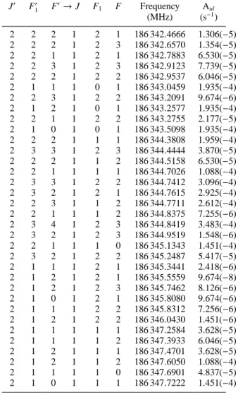
Table 3. Hyperfine components and Aul Einstein spontaneous emission coefficients of the (J:2–1) transition of N2H+. The
fre-quency uncertainty is ± 2.3 kHz for all hyperfine components.
J′ F′ 1 F ′→J F1 F Frequency A ul (MHz) (s−1) 2 2 2 1 2 1 186 342.4666 1.306(−5) 2 2 2 1 2 3 186 342.6570 1.354(−5) 2 2 1 1 2 1 186 342.7883 6.530(−5) 2 2 3 1 2 3 186 342.9123 7.739(−5) 2 2 2 1 2 2 186 342.9537 6.046(−5) 2 1 1 1 0 1 186 343.0459 1.935(−4) 2 2 3 1 2 2 186 343.2091 9.674(−6) 2 1 2 1 0 1 186 343.2577 1.935(−4) 2 2 1 1 2 2 186 343.2755 2.177(−5) 2 1 0 1 0 1 186 343.5098 1.935(−4) 2 2 2 1 1 1 186 344.3808 1.959(−4) 2 3 3 1 2 3 186 344.4444 3.870(−5) 2 2 2 1 1 2 186 344.5158 6.530(−5) 2 2 1 1 1 1 186 344.7026 1.088(−4) 2 3 3 1 2 2 186 344.7412 3.096(−4) 2 3 2 1 2 1 186 344.7615 2.925(−4) 2 2 3 1 1 2 186 344.7711 2.612(−4) 2 2 1 1 1 2 186 344.8375 7.255(−6) 2 3 4 1 2 3 186 344.8419 3.483(−4) 2 3 2 1 2 3 186 344.9519 1.548(−6) 2 2 1 1 1 0 186 345.1343 1.451(−4) 2 3 2 1 2 2 186 345.2487 5.417(−5) 2 1 1 1 2 1 186 345.3441 2.418(−6) 2 1 2 1 2 1 186 345.5559 9.674(−8) 2 1 2 1 2 3 186 345.7462 8.126(−6) 2 1 0 1 2 1 186 345.8080 9.674(−6) 2 1 1 1 2 2 186 345.8312 7.256(−6) 2 1 2 1 2 2 186 346.0430 1.451(−6) 2 1 1 1 1 1 186 347.2584 3.628(−5) 2 1 1 1 1 2 186 347.3933 6.046(−5) 2 1 2 1 1 1 186 347.4701 3.628(−5) 2 1 2 1 1 2 186 347.6050 1.088(−4) 2 1 1 1 1 0 186 347.6901 4.837(−5) 2 1 0 1 1 1 186 347.7222 1.451(−4)
L. Pagani et al.: On the frequency of N2H+and N2D+(RN), Online Material p 2
Table 4. Hyperfine components and Aul Einstein spontaneous emission coefficients of the (J:3–2) transition of N2H+. The
fre-quency uncertainty is ± 11 kHz for all hyperfine components.
J′ F′ 1 F ′→J F1 F Frequency A ul (MHz) (s−1) 3 3 3 2 3 2 279 509.361 1.110(−5) 3 3 3 2 3 4 279 509.471 1.124(−5) 3 3 2 2 3 2 279 509.795 1.244(−4) 3 3 4 2 3 4 279 509.849 1.312(−4) 3 3 3 2 3 3 279 509.868 1.176(−4) 3 3 4 2 3 3 279 510.246 8.745(−6) 3 3 2 2 3 3 279 510.302 1.555(−5) 3 2 2 2 1 2 279 511.103 2.644(−4) 3 2 2 2 1 1 279 511.315 7.933(−4) 3 2 1 2 1 0 279 511.355 5.876(−4) 3 4 4 2 3 4 279 511.384 7.870(−5) 3 3 3 2 2 3 279 511.401 1.244(−4) 3 2 3 2 1 2 279 511.479 1.058(−3) 3 2 1 2 1 2 279 511.607 2.938(−5) 3 3 3 2 2 2 279 511.656 9.950(−4) 3 3 2 2 2 1 279 511.768 9.402(−4) 3 3 4 2 2 3 279 511.778 1.119(−3) 3 4 3 2 3 2 279 511.780 1.156(−3) 3 4 4 2 3 3 279 511.781 1.181(−3) 3 2 1 2 1 1 279 511.819 4.407(−4) 3 4 5 2 3 4 279 511.832 1.259(−3) 3 3 2 2 2 3 279 511.834 4.975(−6) 3 4 3 2 3 4 279 511.890 1.606(−6) 3 2 2 2 3 2 279 511.897 6.218(−7) 3 3 2 2 2 2 279 512.090 1.741(−4) 3 2 3 2 3 2 279 512.273 1.269(−8) 3 4 3 2 3 3 279 512.287 1.012(−4) 3 2 3 2 3 4 279 512.383 5.140(−6) 3 2 1 2 3 2 279 512.401 5.597(−6) 3 2 2 2 3 3 279 512.405 4.975(−6) 3 2 3 2 3 3 279 512.781 4.442(−7) 3 2 2 2 2 1 279 513.870 2.938(−5) 3 2 2 2 2 3 279 513.937 3.047(−5) 3 2 2 2 2 2 279 514.192 1.360(−4) 3 2 3 2 2 3 279 514.313 1.741(−4) 3 2 1 2 2 1 279 514.374 1.469(−4) 3 2 3 2 2 2 279 514.568 2.177(−5) 3 2 1 2 2 2 279 514.696 4.897(−5)
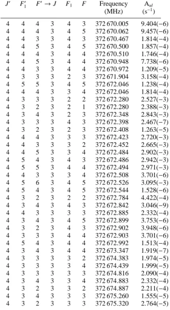
Table 5. Hyperfine components and Aul Einstein spontaneous emission coefficients of the (J:4–3) transition of N2H+. The
fre-quency uncertainty is ± 41 kHz for all hyperfine components.
J′ F′ 1 F ′→J F1 F Frequency A ul (MHz) (s−1) 4 4 4 3 4 3 372 670.005 9.404(−6) 4 4 4 3 4 5 372 670.062 9.457(−6) 4 4 3 3 4 3 372 670.467 1.814(−4) 4 4 5 3 4 5 372 670.500 1.857(−4) 4 4 4 3 4 4 372 670.510 1.746(−4) 4 4 5 3 4 4 372 670.948 7.738(−6) 4 4 3 3 4 4 372 670.972 1.209(−5) 4 3 3 3 2 3 372 671.904 3.158(−4) 4 5 5 3 4 5 372 672.046 1.238(−4) 4 4 4 3 3 4 372 672.046 1.814(−4) 4 3 3 3 2 2 372 672.280 2.527(−3) 4 3 2 3 2 1 372 672.280 2.388(−3) 4 3 4 3 2 3 372 672.348 2.843(−3) 4 3 3 3 4 3 372 672.398 2.467(−7) 4 3 2 3 2 3 372 672.408 1.263(−5) 4 4 4 3 3 3 372 672.423 2.720(−3) 4 4 3 3 3 2 372 672.452 2.665(−3) 4 4 5 3 3 4 372 672.484 2.902(−3) 4 5 4 3 4 3 372 672.486 2.942(−3) 4 5 5 3 4 4 372 672.494 2.971(−3) 4 4 3 3 3 4 372 672.508 3.701(−6) 4 5 6 3 4 5 372 672.526 3.095(−3) 4 5 4 3 4 5 372 672.544 1.528(−6) 4 3 2 3 2 2 372 672.784 4.422(−4) 4 3 4 3 4 3 372 672.842 3.046(−9) 4 4 3 3 3 3 372 672.885 2.332(−4) 4 3 4 3 4 5 372 672.899 3.753(−6) 4 3 2 3 4 3 372 672.902 3.948(−6) 4 3 3 3 4 4 372 672.903 3.701(−6) 4 5 4 3 4 4 372 672.992 1.513(−4) 4 3 4 3 4 4 372 673.347 1.919(−7) 4 3 3 3 3 2 372 674.383 1.974(−5) 4 3 3 3 3 4 372 674.439 1.999(−5) 4 3 3 3 3 3 372 674.816 2.090(−4) 4 3 4 3 3 4 372 674.883 2.332(−4) 4 3 2 3 3 2 372 674.887 2.211(−4) 4 3 4 3 3 3 372 675.260 1.555(−5) 4 3 2 3 3 3 372 675.320 2.764(−5)
L. Pagani et al.: On the frequency of N2H+and N2D+(RN), Online Material p 3
Table 6. Hyperfine components and Aul Einstein spontaneous emission coefficients of the (J:5–4) transition of N2H+. The
fre-quency uncertainty is ± 95 kHz for all hyperfine components.
J′ F′ 1 F ′→J F1 F Frequency A ul (MHz) (s−1) 5 5 5 4 5 4 465 822.236 8.093(−6) 5 5 5 4 5 6 465 822.254 8.118(−6) 5 5 4 4 5 4 465 822.704 2.374(−4) 5 5 6 4 5 6 465 822.729 2.404(−4) 5 5 5 4 5 5 465 822.734 2.311(−4) 5 5 4 4 5 5 465 823.202 9.891(−6) 5 5 6 4 5 5 465 823.209 6.869(−6) 5 4 4 4 3 4 465 824.191 3.673(−4) 5 5 5 4 4 5 465 824.279 2.374(−4) 5 6 6 4 5 6 465 824.285 1.717(−4) 5 4 4 4 5 4 465 824.546 1.221(−7) 5 4 3 4 3 2 465 824.627 5.397(−3) 5 4 4 4 3 3 465 824.635 5.509(−3) 5 4 5 4 3 4 465 824.673 5.877(−3) 5 4 3 4 3 4 465 824.687 7.496(−6) 5 5 5 4 4 4 465 824.717 5.697(−3) 5 5 4 4 4 3 465 824.723 5.642(−3) 5 5 4 4 4 5 465 824.747 2.931(−6) 5 5 6 4 4 5 465 824.754 5.935(−3) 5 6 5 4 5 4 465 824.756 5.978(−3) 5 6 6 4 5 5 465 824.765 6.010(−3) 5 6 5 4 5 6 465 824.774 1.419(−6) 5 6 7 4 5 6 465 824.788 6.182(−3) 5 4 5 4 5 4 465 825.029 1.009(−9) 5 4 3 4 5 4 465 825.042 3.053(−6) 5 4 4 4 5 5 465 825.045 2.931(−6) 5 4 5 4 5 6 465 825.047 2.952(−6) 5 4 3 4 3 3 465 825.131 4.722(−4) 5 5 4 4 4 4 465 825.185 2.901(−4) 5 6 5 4 5 5 465 825.254 2.029(−4) 5 4 5 4 5 5 465 825.527 9.991(−8) 5 4 4 4 4 3 465 826.566 1.469(−5) 5 4 4 4 4 5 465 826.590 1.478(−5) 5 4 4 4 4 4 465 827.028 2.728(−4) 5 4 3 4 4 3 465 827.062 2.833(−4) 5 4 5 4 4 5 465 827.072 2.902(−4) 5 4 5 4 4 4 465 827.510 1.209(−5) 5 4 3 4 4 4 465 827.524 1.889(−5)
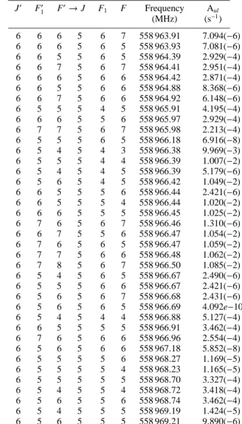
Table 7. Hyperfine components and Aul Einstein spontaneous emission coefficients of the (J:6–5) transition of N2H+. The
fre-quency uncertainty is ± 0.18 MHz for all hyperfine components.
J′ F′ 1 F ′→J F1 F Frequency A ul (MHz) (s−1) 6 6 6 5 6 7 558 963.91 7.094(−6) 6 6 6 5 6 5 558 963.93 7.081(−6) 6 6 5 5 6 5 558 964.39 2.929(−4) 6 6 7 5 6 7 558 964.41 2.951(−4) 6 6 6 5 6 6 558 964.42 2.871(−4) 6 6 5 5 6 6 558 964.88 8.368(−6) 6 6 7 5 6 6 558 964.92 6.148(−6) 6 5 5 5 4 5 558 965.91 4.195(−4) 6 6 6 5 5 6 558 965.97 2.929(−4) 6 7 7 5 6 7 558 965.98 2.213(−4) 6 5 5 5 6 5 558 966.18 6.916(−8) 6 5 4 5 4 3 558 966.38 9.969(−3) 6 5 5 5 4 4 558 966.39 1.007(−2) 6 5 4 5 4 5 558 966.39 5.179(−6) 6 5 6 5 4 5 558 966.42 1.049(−2) 6 6 5 5 5 6 558 966.44 2.421(−6) 6 6 5 5 5 4 558 966.44 1.020(−2) 6 6 6 5 5 5 558 966.45 1.025(−2) 6 7 6 5 6 7 558 966.46 1.310(−6) 6 6 7 5 5 6 558 966.47 1.054(−2) 6 7 6 5 6 5 558 966.47 1.059(−2) 6 7 7 5 6 6 558 966.48 1.062(−2) 6 7 8 5 6 7 558 966.50 1.085(−2) 6 5 4 5 6 5 558 966.67 2.490(−6) 6 5 5 5 6 6 558 966.67 2.421(−6) 6 5 6 5 6 7 558 966.68 2.431(−6) 6 5 6 5 6 5 558 966.69 4.092e−10 6 5 4 5 4 4 558 966.88 5.127(−4) 6 6 5 5 5 5 558 966.91 3.462(−4) 6 7 6 5 6 6 558 966.96 2.554(−4) 6 5 6 5 6 6 558 967.18 5.852(−8) 6 5 5 5 5 6 558 968.27 1.169(−5) 6 5 5 5 5 4 558 968.23 1.165(−5) 6 5 5 5 5 5 558 968.70 3.327(−4) 6 5 4 5 5 4 558 968.72 3.418(−4) 6 5 6 5 5 6 558 968.74 3.462(−4) 6 5 4 5 5 5 558 969.19 1.424(−5) 6 5 6 5 5 5 558 969.21 9.890(−6)
L. Pagani et al.: On the frequency of N2H+and N2D+(RN), Online Material p 4
Table 8. Hyperfine components and Aul Einstein spontaneous emission coefficients of the (J:1–0) transition of N2D+. The
fre-quency uncertainty is ± 2.8 kHz for all hyperfine components.
J′ F′ 1 F ′→J F1 F Frequency A ul (MHz) (s−1) 1 1 0 0 1 1 77 107.4757 2.056(−5) 1 1 2 0 1 2 77 107.7671 1.542(−5) 1 1 2 0 1 1 77 107.7671 5.140(−6) 1 1 1 0 1 1 77 107.9023 5.140(−6) 1 1 1 0 1 0 77 107.9023 6.854(−6) 1 1 1 0 1 2 77 107.9023 8.568(−6) 1 2 2 0 1 1 77 109.3248 1.542(−5) 1 2 2 0 1 2 77 109.3248 5.141(−6) 1 2 3 0 1 2 77 109.6162 2.056(−5) 1 2 1 0 1 0 77 109.8104 1.142(−5) 1 2 1 0 1 2 77 109.8104 5.712(−7) 1 2 1 0 1 1 77 109.8104 8.568(−6) 1 0 1 0 1 2 77 112.1085 1.142(−5) 1 0 1 0 1 0 77 112.1085 2.285(−6) 1 0 1 0 1 1 77 112.1085 6.855(−6)
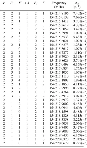
Table 9. Hyperfine components and Aul Einstein spontaneous emission coefficients of the (J:2–1) transition of N2D+. The
fre-quency uncertainty is ± 2.1 kHz for all hyperfine components
J′ F′ 1 F ′→J F1 F Frequency A ul (MHz) (s−1) 2 2 2 1 2 1 154 214.8196 7.402(−6) 2 2 2 1 2 3 154 215.0138 7.676(−6) 2 2 1 1 2 1 154 215.1417 3.701(−5) 2 2 3 1 2 3 154 215.2619 4.387(−5) 2 2 2 1 2 2 154 215.3052 3.427(−5) 2 1 1 1 0 1 154 215.3991 1.097(−4) 2 2 3 1 2 2 154 215.5533 5.483(−6) 2 1 2 1 0 1 154 215.6021 1.097(−4) 2 2 1 1 2 2 154 215.6273 1.234(−5) 2 1 0 1 0 1 154 215.8617 1.097(−4) 2 2 2 1 1 1 154 216.7277 1.110(−4) 2 3 3 1 2 3 154 216.7920 2.193(−5) 2 2 2 1 1 2 154 216.8629 3.701(−5) 2 2 1 1 1 1 154 217.0498 6.169(−5) 2 3 3 1 2 2 154 217.0834 1.755(−4) 2 3 2 1 2 1 154 217.1055 1.658(−4) 2 2 3 1 1 2 154 217.1110 1.481(−4) 2 3 4 1 2 3 154 217.1807 1.974(−4) 2 2 1 1 1 2 154 217.1850 4.113(−6) 2 3 2 1 2 3 154 217.2998 8.773(−7) 2 2 1 1 1 0 154 217.4764 8.225(−5) 2 3 2 1 2 2 154 217.5912 3.071(−5) 2 1 1 1 2 1 154 217.6972 1.371(−6) 2 1 2 1 2 1 154 217.9002 5.483(−8) 2 1 2 1 2 3 154 218.0944 4.606(−6) 2 1 0 1 2 1 154 218.1598 5.483(−6) 2 1 1 1 2 2 154 218.1828 4.113(−6) 2 1 2 1 2 2 154 218.3858 8.225(−7) 2 1 1 1 1 1 154 219.6053 2.056(−5) 2 1 1 1 1 2 154 219.7405 3.427(−5) 2 1 2 1 1 1 154 219.8083 2.056(−5) 2 1 2 1 1 2 154 219.9435 6.169(−5) 2 1 1 1 1 0 154 220.0320 2.742(−5) 2 1 0 1 1 1 154 220.0679 8.225(−5)
Table 10. Hyperfine components and AulEinstein spontaneous emission coefficients of the (J:3–2) transition of N2D+. The
fre-quency uncertainty is ± 6.2 kHz for all hyperfine components
J′ F′ 1 F ′→J F1 F Frequency A ul (MHz) (s−1) 3 3 3 2 3 2 231 319.4552 6.294(−6) 3 3 3 2 3 4 231 319.5743 6.373(−6) 3 3 2 2 3 2 231 319.8904 7.049(−5) 3 3 4 2 3 4 231 319.9411 7.435(−5) 3 3 3 2 3 3 231 319.9629 6.664(−5) 3 3 4 2 3 3 231 320.3297 4.957(−6) 3 3 2 2 3 3 231 320.3981 8.812(−6) 3 2 2 2 1 2 231 321.1993 1.499(−4) 3 2 2 2 1 1 231 321.4023 4.497(−4) 3 2 1 2 1 0 231 321.4445 3.331(−4) 3 4 4 2 3 4 231 321.4756 4.461(−5) 3 3 3 2 2 3 231 321.4930 7.050(−5) 3 2 3 2 1 2 231 321.5630 5.996(−4) 3 2 1 2 1 2 231 321.7041 1.665(−5) 3 3 3 2 2 2 231 321.7411 5.640(−4) 3 3 2 2 2 1 231 321.8543 5.330(−4) 3 3 4 2 2 3 231 321.8599 6.345(−4) 3 4 4 2 3 3 231 321.8643 6.692(−4) 3 4 3 2 3 2 231 321.8645 6.555(−4) 3 2 1 2 1 1 231 321.9071 2.498(−4) 3 4 5 2 3 4 231 321.9120 7.138(−4) 3 3 2 2 2 3 231 321.9283 2.820(−6) 3 4 3 2 3 4 231 321.9836 9.104(−7) 3 2 2 2 3 2 231 321.9940 3.525(−7) 3 3 2 2 2 2 231 322.1764 9.870(−5) 3 2 3 2 3 2 231 322.3577 7.194(−9) 3 4 3 2 3 3 231 322.3722 5.736(−5) 3 2 3 2 3 4 231 322.4768 2.913(−6) 3 2 1 2 3 2 231 322.4988 3.172(−6) 3 2 2 2 3 3 231 322.5017 2.820(−6) 3 2 3 2 3 3 231 322.8654 2.518(−7) 3 2 2 2 2 1 231 323.9578 1.666(−5) 3 2 2 2 2 3 231 324.0318 1.727(−5) 3 2 2 2 2 2 231 324.2799 7.711(−5) 3 2 3 2 2 3 231 324.3955 9.870(−5) 3 2 1 2 2 1 231 324.4626 8.328(−5) 3 2 3 2 2 2 231 324.6436 1.234(−5) 3 2 1 2 2 2 231 324.7847 2.776(−5)
L. Pagani et al.: On the frequency of N2H+and N2D+(RN), Online Material p 5
Table 11. Hyperfine components and Aul Einstein spontaneous emission coefficients of the (J:4–3) transition of N2D+. The
fre-quency uncertainty is ± 25 kHz for all hyperfine components
J′ F′ 1 F ′→J F1 F Frequency A ul (MHz) (s−1) 4 4 4 3 4 3 308 419.723 5.330(−6) 4 4 4 3 4 5 308 419.794 5.361(−6) 4 4 3 3 4 3 308 420.188 1.028(−4) 4 4 5 3 4 5 308 420.218 1.053(−4) 4 4 4 3 4 4 308 420.231 9.896(−5) 4 4 5 3 4 4 308 420.655 4.386(−6) 4 4 3 3 4 4 308 420.696 6.853(−6) 4 3 3 3 2 3 308 421.627 1.790(−4) 4 5 5 3 4 5 308 421.764 7.018(−5) 4 4 4 3 3 4 308 421.765 1.028(−4) 4 3 3 3 2 2 308 421.991 1.432(−3) 4 3 2 3 2 1 308 421.993 1.353(−3) 4 3 4 3 2 3 308 422.056 1.611(−3) 4 3 3 3 4 3 308 422.120 1.399(−7) 4 4 4 3 3 3 308 422.132 1.542(−3) 4 3 2 3 2 3 308 422.134 7.161(−6) 4 4 3 3 3 2 308 422.162 1.511(−3) 4 4 5 3 3 4 308 422.189 1.645(−3) 4 5 4 3 4 3 308 422.195 1.668(−3) 4 5 5 3 4 4 308 422.200 1.684(−3) 4 5 6 3 4 5 308 422.230 1.754(−3) 4 4 3 3 3 4 308 422.231 2.098(−6) 4 5 4 3 4 5 308 422.266 8.664(−7) 4 3 2 3 2 2 308 422.498 2.506(−4) 4 3 4 3 4 3 308 422.549 1.727(−9) 4 4 3 3 3 3 308 422.598 1.322(−4) 4 3 4 3 4 5 308 422.621 2.127(−6) 4 3 2 3 4 3 308 422.628 2.238(−6) 4 3 3 3 4 4 308 422.628 2.098(−6) 4 5 4 3 4 4 308 422.703 8.577(−5) 4 3 4 3 4 4 308 423.057 1.088(−7) 4 3 3 3 3 2 308 424.094 1.119(−5) 4 3 3 3 3 4 308 424.163 1.133(−5) 4 3 3 3 3 3 308 424.530 1.185(−4) 4 3 4 3 3 4 308 424.592 1.322(−4) 4 3 2 3 3 2 308 424.602 1.253(−4) 4 3 4 3 3 3 308 424.959 8.812(−6) 4 3 2 3 3 3 308 425.037 1.567(−5)
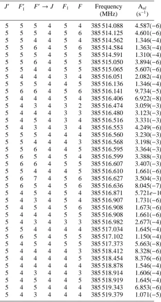
Table 12. Hyperfine components and AulEinstein spontaneous emission coefficients of the (J:5–4) transition of N2D+. The
fre-quency uncertainty is ± 58 kHz for all hyperfine components
J′ F′ 1 F ′→J F1 F Frequency A ul (MHz) (s−1) 5 5 5 4 5 4 385 514.088 4.587(−6) 5 5 5 4 5 6 385 514.125 4.601(−6) 5 5 4 4 5 4 385 514.562 1.346(−4) 5 5 6 4 5 6 385 514.584 1.363(−4) 5 5 5 4 5 5 385 514.591 1.310(−4) 5 5 6 4 5 5 385 515.050 3.894(−6) 5 5 4 4 5 5 385 515.065 5.607(−6) 5 4 4 4 3 4 385 516.051 2.082(−4) 5 5 5 4 4 5 385 516.136 1.346(−4) 5 6 6 4 5 6 385 516.141 9.734(−5) 5 4 4 4 5 4 385 516.406 6.922(−8) 5 4 3 4 3 2 385 516.474 3.059(−3) 5 4 4 4 3 3 385 516.480 3.123(−3) 5 4 5 4 3 4 385 516.516 3.331(−3) 5 4 3 4 3 4 385 516.553 4.249(−6) 5 5 5 4 4 4 385 516.560 3.230(−3) 5 5 4 4 4 3 385 516.568 3.198(−3) 5 5 6 4 4 5 385 516.595 3.364(−3) 5 6 5 4 5 4 385 516.599 3.388(−3) 5 6 6 4 5 5 385 516.607 3.407(−3) 5 5 4 4 4 5 385 516.610 1.661(−6) 5 6 7 4 5 6 385 516.627 3.504(−3) 5 6 5 4 5 6 385 516.636 8.045(−7) 5 4 5 4 5 4 385 516.871 5.721e−10 5 4 3 4 5 4 385 516.907 1.731(−6) 5 4 5 4 5 6 385 516.908 1.673(−6) 5 4 4 4 5 5 385 516.908 1.661(−6) 5 4 3 4 3 3 385 516.982 2.677(−4) 5 5 4 4 4 4 385 517.034 1.645(−4) 5 6 5 4 5 5 385 517.102 1.150(−4) 5 4 5 4 5 5 385 517.373 5.663(−8) 5 4 4 4 4 3 385 518.412 8.328(−6) 5 4 4 4 4 5 385 518.454 8.376(−6) 5 4 4 4 4 4 385 518.878 1.546(−4) 5 4 3 4 4 3 385 518.914 1.606(−4) 5 4 5 4 4 5 385 518.919 1.645(−4) 5 4 5 4 4 4 385 519.343 6.853(−6) 5 4 3 4 4 4 385 519.379 1.071(−5)
L. Pagani et al.: On the frequency of N2H+and N2D+(RN), Online Material p 6
Table 13. Hyperfine components and Aul Einstein spontaneous emission coefficients of the (J:6–5) transition of N2D+. The
fre-quency uncertainty is ± 0.11 MHz for all hyperfine components
J′ F′ 1 F ′→J F1 F Frequency A ul (MHz) (s−1) 6 6 6 5 6 5 462 601.05 4.014(−6) 6 6 6 5 6 7 462 601.06 4.021(−6) 6 6 5 5 6 5 462 601.53 1.660(−4) 6 6 7 5 6 7 462 601.54 1.673(−4) 6 6 6 5 6 6 462 601.55 1.627(−4) 6 6 5 5 6 6 462 602.02 4.744(−6) 6 6 7 5 6 6 462 602.03 3.485(−6) 6 5 5 5 4 5 462 603.04 2.378(−4) 6 6 6 5 5 6 462 603.10 1.660(−4) 6 7 7 5 6 7 462 603.11 1.255(−4) 6 5 5 5 6 5 462 603.32 3.920(−8) 6 5 4 5 4 3 462 603.50 5.651(−3) 6 5 5 5 4 4 462 603.51 5.707(−3) 6 5 6 5 4 5 462 603.53 5.945(−3) 6 5 4 5 4 5 462 603.54 2.936(−6) 6 6 5 5 5 4 462 603.56 5.780(−3) 6 6 6 5 5 5 462 603.56 5.811(−3) 6 6 5 5 5 6 462 603.58 1.372(−6) 6 6 7 5 5 6 462 603.59 5.977(−3) 6 7 6 5 6 5 462 603.59 6.002(−3) 6 7 7 5 6 6 462 603.60 6.022(−3) 6 7 6 5 6 7 462 603.60 7.424(−7) 6 7 8 5 6 7 462 603.61 6.148(−3) 6 5 6 5 6 5 462 603.81 2.320e−10 6 5 4 5 6 5 462 603.81 1.411(−6) 6 5 5 5 6 6 462 603.81 1.372(−6) 6 5 6 5 6 7 462 603.81 1.378(−6) 6 5 4 5 4 4 462 604.00 2.906(−4) 6 6 5 5 5 5 462 604.04 1.962(−4) 6 7 6 5 6 6 462 604.09 1.448(−4) 6 5 6 5 6 6 462 604.30 3.317(−8) 6 5 5 5 5 4 462 605.35 6.605(−6) 6 5 5 5 5 6 462 605.37 6.626(−6) 6 5 5 5 5 5 462 605.83 1.886(−4) 6 5 4 5 5 4 462 605.85 1.938(−4) 6 5 6 5 5 6 462 605.86 1.962(−4) 6 5 6 5 5 5 462 606.32 5.606(−6) 6 5 4 5 5 5 462 606.32 8.073(−6)