HAL Id: hal-00591124
https://hal.archives-ouvertes.fr/hal-00591124
Submitted on 14 Apr 2021
HAL is a multi-disciplinary open access
archive for the deposit and dissemination of
sci-entific research documents, whether they are
pub-lished or not. The documents may come from
teaching and research institutions in France or
abroad, or from public or private research centers.
L’archive ouverte pluridisciplinaire HAL, est
destinée au dépôt et à la diffusion de documents
scientifiques de niveau recherche, publiés ou non,
émanant des établissements d’enseignement et de
recherche français ou étrangers, des laboratoires
publics ou privés.
Gregory Beaugrand, Sylvain Lenoir, F. Ibañez, Claude Manté
To cite this version:
Gregory Beaugrand, Sylvain Lenoir, F. Ibañez, Claude Manté. A new model to assess the probability of
occurrence of a species, based on presence-only data. Marine Ecology Progress Series, Inter Research,
2011, 424, pp.175-190. �10.3354/meps08939�. �hal-00591124�
INTRODUCTION
The effects of climate change on living systems in both the terrestrial and the marine realms are now well documented (Parmesan & Matthews 2006, IPCCWG1 2007a). In the marine biosphere, current climate change is affecting the abundance, spatial distribution and phenology of species, as well as altering prey-predator interactions (Beaugrand et al. 2002,
Beau-grand et al. 2003, Edwards & Richardson 2004). The effect of climate change is seen from phytoplankton (Reid et al. 1998) to zooplankton (Beaugrand et al. 2007) and fish (Brander et al. 2003, Perry et al. 2005), and it translates from the physiological to the ecosys-tem level (Pörtner & Farrell 2008), affecting coupling between systems (i.e. bentho-pelagic coupling; Reid & Edwards 2001, Kirby et al. 2008). Pronounced climate change may become a confounding factor of fishing,
© Inter-Research 2011 · www.int-res.com *Email: Gregory.Beaugrand@univ-lille1.fr
A new model to assess the probability of
occurrence of a species, based on presence-only data
G. Beaugrand
1, 2,*, S. Lenoir
1, F. Ibañez
3, C. Manté
41Centre National de la Recherche Scientifique, Laboratoire d’Océanologie et de Géosciences UMR LOG CNRS 8187,
Station Marine, Université des Sciences et Technologies de Lille – Lille 1, BP 80, 62930 Wimereux, France
2Sir Alister Hardy Foundation for Ocean Science, The Laboratory, Citadel Hill, Plymouth PL1 2PB, UK 3Laboratoire d’Oceanographie de Villefranche (LOV) BP 28, 06234 Villefranche-sur-Mer CEDEX, France
4Centre d’Océanologie de Marseille, UMR CNRS 6117 LMGEM, Campus de Luminy, Case 901, 13288 Marseille CEDEX 09,
France
ABSTRACT: This study aims to describe a new nonparametric ecological niche model for the analy-sis of presence-only data, which we use to map the spatial distribution of Atlantic cod and to project the potential impact of climate change on this species. The new model, called the Non-Parametric Probabilistic Ecological Niche (NPPEN) model, is derived from a test recently applied to compare the ecological niche of 2 different species. The analysis is based on a simplification of the Multiple Response Permutation Procedures (MRPP) using the Generalised Mahalanobis distance. For the first time, we propose to test the generalized Mahalanobis distance by a non-parametric procedure, thus avoiding the arbitrary selection of quantile classes to allow the direct estimation of the probability of occurrence of a species. The model NPPEN was applied to model the ecological niche (sensu Hutchinson) of Atlantic cod and therefore its spatial distribution. The modelled niche exhibited high probabilities of occurrence at bathymetry ranging from 0 to 500 m (mode from 100 to 300 m), at annual sea surface temperature of from –1 to 14°C (mode from 4 to 8°C) and at annual sea surface salinity ranging from 0 to 36 (mode from 25 to 34). This made the species a good indicator of the sub-arctic province. Current climate change is having a strong effect on North Sea cod and may have also reinforced the negative impact of fishing on stocks located offshore of North America. The model shows a pronounced effect of present-day climate change on the spatial distribution of Atlantic cod. Projections for the coming decades suggest that cod may eventually disappear as a commercial spe-cies from regions where a sustained decrease or collapse has already been documented. In contrast, the abundance of cod is likely to increase in the Barents Sea.
KEY WORDS: Ecological niche models · Multiple response permutation procedure · Generalised Mahalanobis distance · Atlantic cod
and both climate change and fishing may act in syn-ergy to precipitate the collapse of fish stocks around the world (Beaugrand & Kirby 2010b,a). To better eval-uate the effect of climate on a species, it is essential to know its spatial distribution; this information is often lacking in the marine realm.
One way to evaluate the spatial distribution of a spe-cies is to use Ecological Niche Models (ENMs). ENMs, also known as bioclimatic envelopes, are being more frequently used in the context of global change and are often based on the concept of the ecological realised niche described by Hutchinson (1957). The realised niche is the environmental envelope in which a species can be found when the effect of dispersal and interspe-cific relationships are considered. ENMs have been used in conservation to manage endangered species (Sanchez-Cordero et al. 2005), to predict the responses of species to climate change (Berry et al. 2002), to fore-cast past distribution (Bigg et al. 2008) and to estimate the potential invasion of a non-native species (Peterson & Vieglais 2001). When quantitative data are available, regression techniques such as Generalised Linear Models (GLMs; McCullagh & Nelder 1983) or Gener-alised Additive Models (GAMs; Hastie & Tibshirani 1990), ordination or neural networks have been fre-quently used (Guisan & Zimmermann 2000, Guisan & Thuiller 2005). When only binary (presence-absence) data are available there are far fewer techniques that can be applied, although regression techniques such as GAMs can still be utilised. Traditional models such as BIOCLIM (based on a multilevel rectilinear enve-lope) and DOMAIN (based on a point-to-point similar-ity metric; Carpenter et al. 1993) tend to be relatively simple, although more sophisticated models have been developed recently, such as Ecological Niche Factor Analysis (ENFA, (Hirzel et al. 2002) and MAXENT (Phillips et al. 2006), which are based upon Principal Component Analysis (PCA) and the principle of maxi-mum entropy, respectively.
The objective of this study is to describe a new nonparametric ENM adapted to presence-only data. This technique is based on a modified version of the Multiple Response Permutation Procedure (MRPP; Mielke et al. 1981), using the Generalised Maha-lanobis distance (Ibañez 1981). (1) We present a ratio-nale and describe the technique. (2) We present a simple example of a calculation based on simulated data in order to illustrate the technique and to justify the use of the generalised Mahalanobis distance. (3) We use the technique to model the ecological niche of the Atlantic cod and map its probability of rence. Then we project the probability of cod occur-rence for the middle and the end of the 21st century based upon IPCC scenarios for changes in sea surface temperature.
MATERIALS AND METHODS Physical data
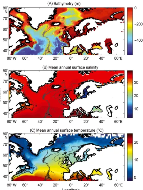
Bathymetry data were obtained from a global ocean bathymetry chart (1° longitude × 1° latitude; Smith & Sandwell 1997). This dataset is among the most com-plete, high-resolution image of sea floor topography currently available. The chart was constructed from data obtained from ships with detailed gravity-anomaly information provided by the satellites GEOSAT and ERS-1 (Smith & Sandwell 1997). Bathymetry data were considered because the spatial distribution of Atlantic cod, which occurs mainly over continental shelves (Sundby 2000), is explained partially by this parameter. Salinity has a strong impact upon the distribution of most fishes. Annual Sea Surface Salinity (SSS) data for a depth ranging from 0 to 10 m, were obtained from the Levitus climatology (Levitus 1982). International Council for the Exploration of the Sea (ICES) data were used to complete the Levitus dataset in coastal regions (e.g. some regions of the eastern English Channel) where there was no assessment of annual SSS. ICES data were downloaded from www.ices.dk. We did not include temporal changes in salinity because the para-meter is not presently well assessed in the Atmos-phere-Ocean General Circulation (AO-GCM) models (M. Visbeck, pers. comm.). Furthermore, the spatial variance in the salinity is much more pronounced than the temporal variance.
The spatial distribution of cod is affected by temper-ature (Brander 2000, ICES 2007). Sea Surface Temper-ature (SST) data from 1960 to 2005 were taken from the International Comprehensive Ocean-Atmosphere Data Set (ICOADS) at http://icoads.noaa.gov. Longi-tudes had a spatial resolution of 1° longitude × 1° lati-tude (Woodruff et al. 1987). An annual mean was cal-culated for the period from 1960 to 2005. SST data were considered, as this parameter has a strong effect on the spatial distribution of cod (Brander 2000, ICES 2007). The use of SST to assess the niche of adult cod assumes that climate exerts its major influence on cod through the effects of temperature on larval develop-ment and plankton food availability, since the pelagic larval stage is a critical life cycle phase affecting re-cruitment (Beaugrand & Kirby 2010b,a).
To assess the potential effect of changes in SST, data were obtained for the period 1990 to 2100 from the AO-GCM ECHAM 4 (EC = European Centre and HAM = Hamburg; Roeckner et al. 1996). These data are projections of monthly skin-temperature equiva-lent above the sea to SST (http://ipcc-ddc.cru.uea. ac.uk). Data used here are modelled based on scenario A2 of the IPCC Special Report on Emissions Scenarios (SRES), which scenario has the atmospheric
concentra-tion of CO2 reaching 856 ppm by 2100, and on SRES
scenario B2, where atmospheric CO2reaches 621 ppm
by 2100 (IPCCWG1 2007b). Scenario A2 supposes a rate of increase of CO2 similar to that currently
ob-served. SRES scenarios A2 and B2 reflect world popu-lations of 15.1 and 10.4 billion people in 2100, respec-tively (IPCCWG1 2007b).
We also used data from the Hadley Centre Coupled Model, version 3 (HadCM3; Gordon et al. 2000). Data were used from both SRES scenarios A1B and B1. Sce-nario A1B reflects a world of rapid economic growth, low population growth and rapid introduction of new and more efficient technology, whereas scenario B1 re-flects a world with rapid introduction of resource-effi-cient technologies (IPCCWG1 2007b). Two non-SRES scenarios were also utilised: PICNTRL (i.e. experiments run with constant pre-industrial levels of greenhouse gasses) and COMMIT (i.e. idealised
sce-nario in which the atmospheric burdens of long-lived greenhouse gasses are held fixed at the 2000 level). The Hadley Centre Global Environmental Model, version 1 (HadGEM1), was also used with the non-SRES scenario 1PTO4x (1% to quadruple) in which greenhouse gasses increase from pre-industrial levels at a rate of 1% per year until the concentration has quadrupled and becomes constant thereafter (Johns et al. 2006). This is the most pessimistic of all sce-narios we considered. In sum, a total of 7 scenarios (A2, B2, A1B, B1, PICNTRL, COMMIT and 1PTO4x) was used from 3 different AO-GCMs (ECHAM4, HadCM3, HadGEM1). The best estimate of global temperature increase is 0.6°C for COMMIT, 1.8°C for Scenario B1, 2.4°C for Scenario B2, 2.8°C for Scenario A1B and 3.4°C for Scenario A2 (IPCCWG1 2007b). These fore-casted SST datasets were used (1) to exam-ine how the probability of occurrence of cod varied as a function of the intensity of warming and AO-GCMs and (2) to identify regions most susceptible to the influence of intense warming.
All physical data were interpolated bilin-early on a spatial grid of 0.1° longitude × 0.1° latitude in a spatial domain ranging from 80.50°W to 70.50°E and from 35.50° N to 70.50° N (Fig. 1). We used a high spatial resolution to decrease potential bias that could arise from the averaging of bathy-metry data in a large geographical cell. The high resolution also enabled us to better assess the probability of cod occur-rence along coastline. While only one map
of bathymetry and SSS (annual climatology) was gen-erated, a grid for each year of the period from 1960 to 2006 was built for SST. Therefore, the spatial distribu-tion of cod varies according to the 3 abiotic parameters, while year-to-year changes were a function of SST only.
Fish data
Data of cod occurrence were taken from Fishbase (www.fishbase.org; Froese & Pauly 2009). This repre-sented a total of 52630 data points. Unfortunately, while high densities of data are present in the dataset on the western side of the North Atlantic this is not the case on the eastern side. Of the 52630 data points taken from Fishbase, only 9638 were located to the east of 30° W. Therefore, we completed the dataset from our
knowl-Fig. 1. Spatial distribution of (A) bathymetry, (B) mean annual sea surface salinity and (C) mean annual sea surface temperature. Isobaths: grey lines
edge of the spatial distribution of the species (ICES 2005, Brander et al. 2006, Heath & Lough 2007, ICES 2007) (Fig. 2). The data largely reflect the occurrence of cod over 1 yr (www.fishbase.org), although no distinction was made on age. Data therefore originated from scien-tific cruises, agencies, museums, university, nongovern-mental organizations, commercial catches, occasional fishermen and expert knowledge. The total number of data points equalled 140026 observations. For each observation of cod occurrence, information on SST, bathymetry and SSS were added to each data point by interpolation of each environmental data point from the datasets described above (see section on physical data). To compare results of our ecological niche model, we used probability data of cod occurrence obtained from the numerical procedure Aquamaps (www. fishbase.org). This derives from the Relative Environ-mental Suitability (RES) model that was initially devel-oped for mapping mammalian species distribution (Kaschner et al. 2006) and that has been adapted sub-sequently to map the probability of occurrence of all marine organisms. A total of 62 160 data points were used to produce the probability map. Although no dis-tinction was made on age, the data reflect mainly the occurrence of cod ≥1 yr old (www.fishbase.org).
Description of the Non Parametric Probabilistic Ecological Niche (NPPEN) model
The model is derived from a test recently applied to compare the ecological niche of 2 species (Beaugrand
& Helaouët 2008). The analysis is based on Multiple Response Permutation Procedures (MRPP), a test first proposed by Mielke et al. (1981). MRPP has been applied in conjunction with Split Moving Window Boundary analysis to detect discontinuities in time series (Cornelius & Reynolds 1991). This method has also been used to identify abrupt ecosystem shifts (Beaugrand 2004, Beaugrand & Ibañez 2004). Mathematically, MRPP tests whether 2 groups of observations in a multivariate space are significantly separated. Mielke et al. (1981) gave a full description of the test and Beaugrand & Helaouët (2008) have recently illustrated an adaptation of the test to compare 2 ecological niches.
The model we propose for assessing the probability of cod occurrence (and its changes in space and time) is in fact a simplification of MRPP. Instead of comparing 2 groups of observations, our new analysis tests whether one observation belongs to a group of reference observa-tions we call here the reference matrix. The reference matrix is represented by a matrix Xn,pwith n the number
of reference observations and p the number of variables. Each row of the matrix represents the environmental conditions where a species is detected. It is crucial that the reference matrix cover the entire niche of a species to give a reliable probability (Thuiller 2004); we check this point, which is often forgotten in this kind of exer-cise, by compiling histograms. The predictive matrix Ym,p
encompasses m observations of the environment using
p predictors. Each observation of Y (environmental
conditions) is then tested against X (range of conditions where the species was detected). The model is applied in 4 main steps:
Step 1: Homogenization of the reference matrix.
The density of cod occurrence reported in some databases (e.g. Fishbase) depends on fishing activities, and it is clear that the density of data points is higher in fishing areas. Although this suggests that the resource is more abundant in those regions, this is not completely true. This phenomenon can potentially influence the out-come of any ecological niche model. Another phenomenon that can influence probability of occurrence is the inaccurate reporting of occur-rence. In an attempt to overcome these draw-backs, we created a virtual cube (i.e. 3 control-ling factors) with intervals of SST of 1°C between –2°C and 18°C, intervals of bathymetry of 20 m between 0 and 800 m and intervals of annual SSS of 2 between 0 and 40. We retained one data occurrence when more than one observation was made in the crossed intervals of annual SST, bathymetry and annual SSS. This threshold was fixed to eliminate the influence of one single mis-reporting. The resolution might, at first sight, appear to be coarse. However, the practice of the
Fig. 2. Gadus morhua. Spatial distribution of occurrence data points: observed (Fishbase data, 52 630 datapoints, black zones along the coastlines) and inferred (104 642 datapoints, dark grey zones).
ENM indicates that the probability remains similar, even at a lower resolution (see Fig. 4), which depends on the size of the reference matrix. Here, the size was equal to 140 026 observations. This amount divided by 16 000 (20 SST intervals × 40 bathymetric intervals × 20 SSS intervals) = 8.75 observations per geographical cell. Such a calculation obviously assumes that obser-vations are equally distributed, which was clearly not the case. A resolution of 0.1°C for SST, 1 m for bathym-etry and 0.1 unit of SSS would appear to be too sensi-tive, as only 0.02 observations per crossed interval are expected if observations were randomly distributed. The determination of the threshold also depends on the uncertainties of the physical variables.
Step 2: Preparation of data. A matrix called Zn +1,pis
created for each observation of Y to be tested against
X. For the first observation, the following matrix is
con-structed:
(1)
where xi,jis the observation in matrix X and yi,jis an
observation of matrix Y. The building of matrix Z is repeated m times, corresponding to the m observations of Y.
Step 3: Calculation of the mean multivariate dis-tance between the observation to be tested and the reference matrix. MRPP was first proposed for
appli-cation with an Euclidean distance, a squared Euclid-ean distance or a chord distance (Mielke et al. 1981). To first illustrate the technique, we use a Euclidean distance. Obviously, if variables do not have the same unit or dimension, such a distance should be avoided. The Euclidean distance is calculated as follows:
(2) With z1,j the first observations for the j th variable,
originally the observation of the variable of matrix X, 1≤ j ≤ p; zi,j, the observation i of the variable j in matrix
Z with 2 ≤ i ≤ n +1 and 1 ≤ j ≤ p. Then, the average
observed distance εois calculated as follows:
(3) where n, the total number of Euclidean distances, is equal to the number of observations in the training set X.
Step 4: Calculation of the probability that the ob-servation belongs to the reference matrix. The mean
Euclidean distance is tested by replacing each
obser-vation of X by y in Z from row 2 to n +1. The number of maximum permutations is equal to n. After each per-mutation, the mean Euclidean distance εs is
recal-culated, with 1 ≤ s ≤ n. A probability v can be assessed by looking at the number of times a simulated mean Euclidean distance is found to be greater than or equal to the observed mean Euclidean distance between the observation and the reference matrix X.
(4) where the probability v is the number of times the sim-ulated mean Euclidean distance was found greater or equal to the observed mean distance. When v = 1, the observation has environmental conditions that represent the centre of the species niche. When v = 0, the observation has environmental conditions outside the species niche. It is essential to emphasise that the niche and its borders have to be correctly assessed. Applying the procedure to each observation of Ym,p
leads to a matrix Vm,1of probability. It is important to
have a large reference matrix so that the resolution of the probability is as high as possible. The resolution R of the probability is:
(5) where n is the number of reference observations in X. Ideally, R should be < 0.05.
Simple example of application of the model using the Euclidean distance. To illustrate the principle of
the technique, we present a hypothetical case where the reference matrix X has n = 3 observations and v = 2 controlling factors while the predictive matrix Y has
m = 1 observation (Fig. 3). Calculations of the 3
Euclid-ean distances between y and the reference observa-tions x give d(y · x1)= 2.236, d(y · x2)= 2.236 and d(y · x3)=
1.803 (Fig. 3a). The average observed distance εois =
2.092. The simulated distances are εs1= 1.589 (Fig. 3b),
εs2= 1.383 (Fig. 3c) and εs3= 1.140 (Fig. 3d). The
prob-ability is therefore equal to 0. Observation y has envi-ronmental conditions not compatible with the species ecological niche inferred here from 2 variables.
Selection of a better coefficient of distance for Step 2. Mielke et al. (1981) used mainly the
Euclid-ean, squared Euclidean and chord distances. How-ever, in the context of habitat modelling, the use of the Euclidean (squared or not) distance in step 2 is inappropriate in most (if not all) cases and the chord distance is often a better approach (Beaugrand & Helaouët 2008). The computation of the chord dis-tance is achieved by normalizing each vector of Z to 1 prior to the calculation of the Euclidean distances; this is a special kind of scaling (Legendre & Legendre 1998). Each element of the vector is divided by its length, using the Pythagorean formula to ensure that
R n = 1 v q n S = ε ≥ εo εo = =
∑
d n i n 1 1 d z zi z j zi j j p ( 1’ ) ( 1, ,)2 1 = − =∑
Zn p p p n y y y x x x x +1 1 1 1 2 1 1 1 1 2 1 , , , , , , , . . . . . . . . . . . . . . ,,1 xn,2 . . xn p, ⎡ ⎣ ⎢ ⎢ ⎢ ⎢ ⎢ ⎢ ⎤ ⎦ ⎥ ⎥ ⎥ ⎥ ⎥ ⎥each variable carries the same weight in the analysis. In our study, the normalization of elements of Zn +1,p
per Eq. (1) would be:
(6)
where x and y are as in Eq. (1). Here however, we prefer the use of the Mahalanobis generalised dis-tance, which is independent of the scales of the descriptors (as is the chord distance) but which also takes into consideration the covariance (or the corre-lation) among descriptors (Ibañez 1981). The Maha-lanobis generalised distance has been frequently used recently in this context (e.g. Nogués-Bravo et al. 2008). Prior to the calculation of the distance, standardisation of Z is accomplished by the following transformation:
(7) where zijare observation i of the j th variables in Z,
––
Zj
the average value of variable j and Sj the standard
deviation of variable j in Z. To calculate the Maha-lanobis generalized distance between each observa-tion of the environment yi(1 ≤ i ≤ m) and all
observa-tions of the training set xj (1 ≤ j ≤ n), we used a
particular form of the generalized distance, giving the distance between any observation and the centroid of a unique group (Ibañez 1981):
(8) where Rp,pis the correlation matrix of the standardized
table Z* (mean 0 and variance 1), k1,pis the vector of
the differences between values of the p variables at Z*1
of standardized matrix Z* and the mean –Z*i≠1,jof the p
variables in the standardized matrix Z*. Therefore in Step 3, the Euclidean distance was replaced by the use of the Mahalanobis generalised distance.
Analyses
Analysis 1. A comparison of the model based on a
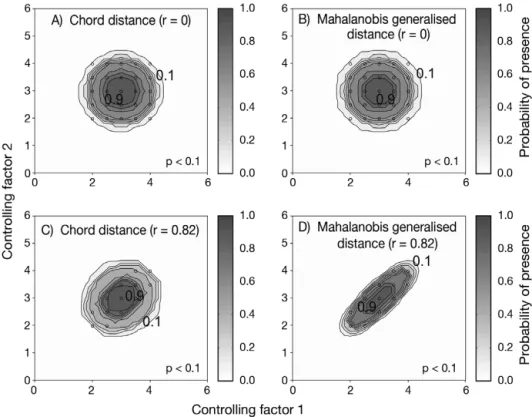
chord distance and the Mahalanobis generalised dis-tance was performed using an example of 2 variables and in 2 cases: no correlation between the 2 variables (r = 0, a training set of 25 observations), and a strong correlation between the 2 variables (r = 0.82, a training set of 13 observations) (Fig. 4).
Dz Z k R k n p 2 1 1, , = ’ − zij zij Zj j * = − S Z y x x y x x n n n * , , , , , , , . . . + = + +…+ 1 1 2 1 1 2 1 1 2 1 1 1 1 1 1 1 ⎡⎡ ⎣ ⎢ ⎢ ⎢ ⎢ ⎢ ⎢ ⎢ ⎢ ⎤ ⎦ ⎥ ⎥ ⎥ ⎥ ⎥ ⎥ ⎥ ⎥
Fig. 3. Principles of the calculation of the niche model that lead to probability of occurrence of a species. (A) Hypothetical obser-vations to be tested against a training set (X) composed of 3 ob-servations in the space of 2 controlling factors. Three Euclidean distances are first calculated and then the average observed dis-tance between the observation to be tested and the ones of the training set is assessed. (B) Recalculation of the mean distance after permutation of the first observation (x1) of the training set
by the observation to be tested. (C) Recalculation of the mean distance after permutation of the second (x2) observation of the
training set by the observation to be tested. (D) Recalculation of the mean distance after permutation of the last observation (x3)
of the training set X by the observation to be tested. All calcu-lated Euclidean distances are indicated by a dashed line. The number of times the simulated mean distance is found inferior to the observed mean distance defines the probability of finding
Analysis 2. The procedure of homogenization was
illustrated by compiling histograms of each predictive variable (annual SST, annual SSS, bathymetry) for all geographical cells of the spatial domain covered by this study, and for both the original and corrected training (or reference) set (Fig. 5).
Analysis 3. The model was then applied to project
the spatial distribution of occurrence of Atlantic cod in order to enable the characterization of its ecological niche (realized niche) as a function of annual SST, annual SSS and bathymetry (Fig. 6). The ecological niche was then projected in the spatial domain as a combined function of the 3 environmental parameters (observed annual SST, annual SSS and bathymetry) for the 1960s and the period from 2000 to 2005 (Fig. 7). Some projections of changes in the spatial distribution of cod occurrence, based on modelled SST (scenarios A2 and B2; annual SSS and bathymetry), were pro-vided for the 1990s (for comparison purposes), the 2050s and the 2090s (Figs. 8 & 9).
RESULTS Analysis 1
A simple example of a training set composed of 2 variables (correlated or not) illustrated well the dif-ference between the chord and the Mahalanobis generalised distances (Fig. 4). When the correlation between 2 parameters was not different from 0, the ecological niche model based on the chord distance and the Mahalanobis generalised distance gave similar results (Fig. 4A,B). However, when the vari-ables of the training set were highly correlated, the model gave improved results when it was based on the Mahalanobis generalised distance (Fig. 4C,D). This fictional example shows that the chord dis-tance should not be used when ecogeographical variables are correlated. Therefore, we did not cal-culate the probability of cod occurrence based on this distance.
Analysis 2
Cod individuals were mainly re-ported over neritic regions (Fig. 5; see also Fig. 2). Most of the reported cod occurrences (79.87% in the original reference matrix) were in regions shallower than 200 m, and the frequency of cod occurrence increased when the region became shallower. The homogenisation procedure did not radically alter the shape of the distribution (Fig. 5). Only a frac-tion of the total records (6.41% of reported cod occurrence) were deeper than 800 m, the threshold of bathymetry selected in this study. The sharpness of the conti-nental slope may explain this small percentage since it is likely that the species can make short incursions over the shelf-edge (small mistakes on the spatial coordinates could increase this percentage slightly). Cod are rarely seen in oceanic regions and some authors have proposed a limit of 600 m, which corresponds to 12.48% of the records (Sundby 2000). To be more conservative, the bathymetric threshold was in-creased to 800 m.
Fig. 4. Fictive examples that show the better performance of the Mahalanobis gener-alised distance in comparison to the chord distance, justifying the choice of the dis-tance coefficient in the ecological niche model NPPEN. First, the reference matrix is composed of 25 observations with 2 controlling factors. The correlation between the 2 controlling factors is null (A and B). (A) Probabilities based on the chord distance (r = 0). (B) Probabilities based on the Mahalanobis generalised distance (r = 0). Second, the reference matrix is composed of 13 observations with 2 parameters. The correlation between the 2 controlling factors is high (r = 0.82; C and D). (C) Probabilities based on the chord distance (r = 0.82). (D) Probabilities based on the Mahalanobis generalised distance (r = 0.82). s= reference observations (reference matrix). High probabilities
are located at the centre of the reference matrix, denoting the centre of the ecological niche (sensu Hutchinson) and probabilities < 0.1 are situated outside (white)
The frequency of occurrence showed a mode over 34 for annual SSS, a mode that corresponds to the one identified when all regions of the Atlantic were taken together. Another smaller mode, more visible after homogenisation, appeared around 8 (Fig. 5). This mode corresponds to the salinity observed in the Baltic Sea. While annual SSTs in the regions of the North Atlantic vary from –2°C to 22°C, with a mode around 2°C, the range of temperature in which cod occurrence was more frequently reported were > 8°C but ranged from 2°C to 14°C in the homogenised reference matrix. The procedure of homogenisation (Step 1) made it clear that the thermal optimum of the species is about 8°C.
Analysis 3
The model NPPEN was first applied to reproduce the ecological niche of Atlantic cod as a function of annual
SST (observed data), annual SSS and bathymetry (Fig. 6). The niche exhibited high probabilities of oc-currence at a bathymetry that ranged between 0 and 500 m (mode between 100 and 300 m), an annual SST of from –1°C to 14°C (mode between 4 and 8°C) and an annual SSS ranging between 0 and 36 (mode between 25 and 34) (Fig. 6).
When projected on the geographical space (Fig. 7), the modelled spatial distribution of the probability of cod occurrence was congruent with the main location of the cod stocks in the North Atlantic sector (Sundby 2000, Bigg et al. 2008). However, there was a notable exception in the Baltic Sea, where low probabilities of cod occurrence were detected (Fig. 7A). A significant decrease in the probability of cod occurrence was evi-dent between the 1960s and the period from 2000 to 2005 in the North Sea, while no such change was noted on the western side of the Atlantic at the southern range of the species’ spatial distribution. At the
north-Fig. 5. Frequency distribution of (A) bathymetry, (B) sea surface salinity (SSS) and (C) sea surface temperature (SST) in the North Atlantic (from 80.50° W to 70.50° E and from 35.50° N to 70.50° N; left panels), in the original reference matrix (i.e. geographical
ern edge of the species’ spatial distribution, probabil-ity of cod occurrence increased along the Greenland coast — especially in the western regions of this coun-try — and in the Barents Sea. Probabilities around the Faeroes and Iceland remained stable.
Probabilities of cod occurrence based on modelled annual SST (ECHAM 4, scenario B2) and observed annual SST were similar (r = 0.95, p < 0.01). However, some discrepancies were noted on the western side of the Atlantic (Fig. 8D; Beaugrand et al. 2008). Based on
modelled data, the probabilities of cod occurrence appear much lower than observed data would suggest during the 1990s on the Georges Bank, the Eastern Scotian Shelf and the Grand Bank (Fig. 8D).
The examination of long-term decadal changes in the probability of cod occurrence projected for this century suggests a clear northward movement of this species (Fig. 9). Interestingly, the probability of cod occurrence decreased substantially at the southern edge of the range of the species: the North Sea, Georges Bank, Eastern Scotian Shelf, Grand Bank and Newfound-land. The probabilities increased in the Barents Sea and in areas close to Greenland, while no major changes were detected for Iceland. The model also suggested a substantial decrease in the probability of cod occurrence around the Faeroes at the end of this century if long-term changes in SST follow Scenario B2 (Fig. 9D).
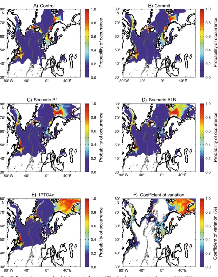
The probability of cod occurrence was sensitive to the intensity of warming (Fig. 10). This sensitivity was not constant in space. Major changes occurred in areas located at the southern or northern limit of the spatial distribution of the species. When the level of anthro-pogenic warming remained unchanged (Fig. 10A,B), the probability of cod occurrence remained high in regions located at the southern limit (and low at the northern limit) of the spatial distribution of the species. However, even with a moderate scenario (Scenario B1, Fig. 10C), the probability of cod occurrence decreased in key regions such as the North Sea and the Georges Bank. When the level of anthropogenic warming in-creased, this had a pronounced influence in regions such as the North Sea and the Eastern Scotian Shelf (Fig. 10D–E). The coefficient of variation calculated per geographical cell using all 7 simulations issued from the 3 models (ECHAM4, HadCM3, HadGEM1) showed the areas where the changes are expected to be the most prominent (Fig. 10F). This analysis showed that modifications are expected to be pronounced at the periphery of the current spatial distribution of spe-cies. High values were observed in the Barents Sea, where a strong increase in the probability of cod occur-rence is expected in the case of an intense warming, and, to a lesser extent, in areas such as the North Sea and the Georges Bank.
DISCUSSION
To predict how the range of marine species may change with climate, it is essential to understand the factors that limit their spatial distributions. One way to achieve this is to use ecological niche models. How-ever, only a limited number of models can deal with presence-only data. The model BIOCLIM use a
recti-Fig. 6. Realised niche (sensu Hutchinson) of the Atlantic cod. Probability of cod occurrence as a function of (A) bathymetry and mean annual sea surface temperature (SST), (B) mean annual sea surface salinity (SSS) and mean annual SST, or (C)
linear volume (Carpenter et al. 1993). The main draw-back of this simple model is the imposed shapes, which can be the cause of a non-justified exclusion or inclu-sion of a geographical point from the predicted distrib-ution (Carpenter et al. 1993). The model DOMAIN can solve this problem by use of a point-to-point similarity metric. However, the metrics used (e.g. the Gower metric; Carpenter et al. 1993, Legendre & Legendre 1998) do not take into account the correlation between descriptors (Legendre & Legendre 1998). Furthermore, a threshold is used to map the modelled distribution of the species. The RES model (Kaschner et al. 2006) uses a trapezoid shape that constitutes a good compromise between species with a shorter or a unimodal eco-logical niche and migratory species with a larger or a
bimodal niche (Kaschner et al. 2006). However, the bounds of this trapezoid need to be precisely defined, implying often arbitrary choices, and thus it requires a good knowledge of the spe-cies. While the Ecological Niche Factor Analysis (ENFA; Hirzel et al. 2002) could be adapted for our study, this technique requires the multinor-mality of the ecogeographical variables to extract the eigenvectors to calculate marginality and specialization factors; for this reason a transformation of the ecogeographical variables (e.g. Box-Cox) is often needed prior to analysis. Finally, the statistical technique MAXENT (Phillips et al. 2006), which is based on the max-imum-entropy principle, also requires accurate threshold definition and shows some applica-tion restricapplica-tions.
NPPEN offers a number of advantages over the above-mentioned methods. Firstly, unlike models such as RES (Kaschner et al. 2006) or the mixed model of Cheung and colleagues (Che-ung et al. 2008), our simple model does not need an a priori knowledge of the species biology. Our technique is also based on a non-paramet-ric test that does not require the multinormality of ecogeographical variables. Although the use of the Generalised Mahalanobis distance is not new in this kind of model (Farber & Kadmon 2003, Cayuela 2004, Etherington et al. 2009), this is the first time that this distance metric has been embedded into a non-parametric test. For example, Cayuela (2004) rescaled the Maha-lanobis distance into quantiles to produce a map of probability, and Nogués-Bravo et al. (2008) converted the distance into quartiles. Ibañez (1981) and Farber & Kadmon (2003) tested this distance by approximating this measure by a χ2 distribution with n-1 degrees of freedom.
Legendre & Legendre (1998) also described the conversion of the D2 by the Hotelling T2 (Hotelling 1931) statistic and its test by the F statistic. These tests require the distribution to be multinormal. Although these authors stated that the test can tolerate some degrees of deviation from this assumption, it can be seen from histograms that the bathymetry data (Fig. 5) were very far from the normality. Finally, the procedure does not need the selection of arbitrary thresholds and is fully statistical. The technique simply tests whether an observation belongs to a group of observations, called here a training set, or a reference matrix. NPPEN therefore can be used very quickly as an exploratory analysis to give a first approximation of the spatial distribution of a species. The test is also appropriate for many species for which no information on its physiology exists. The only caveat is that our
Fig. 7. Modelled spatial distribution in the probability of cod occurrence for the periods (A) 1960–1969 and (B) 2000–2005
model, like others, does not fully resolve the problem of autocorrelation (SAR). The spatial autocorrelation can inflate significantly the probabilities inferred from ENMs (Bahn & McGill 2007). We think that the pres-ence-only technique of ENMs is much less subject to this problem than other types of ENMs (e.g. GLMs). The problem is that only a few studies have considered local functions of autocorrelation (Beaugrand & Ibañez 2002, Dormann et al. 2007). Most corrections applied are based on the global function of autocorrelation with an underlying assumption of isotropy (e.g. Moran’s Index, global semi-variograms), which is rarely the case in biogeography (Beaugrand & Ibañez 2002).
Our technique is currently restricted to presence-only data. Although some adjustments could be made
in the application of the method (e.g. calculating the test for a different category of abundance), it is proba-bly preferable in such a case to use other techniques such as GLMs (McCullagh & Nelder 1983) or GAMs (Hastie & Tibshirani 1990). Guisan & Zimmermann (2000) provided an extensive review of different tech-niques used to assess the spatial distribution of a spe-cies. Another limitation of this technique may lie in the fact that it should only be employed with a limited number of ecogeographical variables. If a high number of variables are used it would be preferable to use a principal component analysis prior to the application of the test, or use the Mahalanobis distance factor analy-sis (MADIFA; Calenge et al. 2008) to better understand the contribution of the ecogeographical variables. This
Fig. 8. Modelled spatial distribution in the probability of cod occurrence for the period 1990–1999. (A) From modelled annual SST (ECHAM 4, scenario B2). (B) From observed annual SST. (C) Relationships between probabilities based on observed and mod-elled (ECHAM 4, scenario B2) annual SST. The Pearson coefficient of correlation is indicated. Probabilities assessed from Sce-nario A2 gave similar conclusions. (D) Difference between probability of cod occurrence based on modelled SST (A) and
can also be done a posteriori by calculating the corre-lation—here the rank correlation coefficient of Spear-man or Kendall (Legendre & Legendre 1998) between the modeled probability and each environmental fac-tor. NPPEN might also be subjected to what might be described as a ‘border effect’. Indeed, the modelling of the niche of Atlantic cod (see Fig. 6) showed a reduc-tion in the probability of cod occurrence towards shal-low regions, which is unexpected based upon our knowledge of the species (Sundby 2000). Indeed, the technique works in such a way that maximum proba-bility is concentrated towards the middle of the niche. Therefore some borders of the multidimensional niche might be underestimated. Although this problem is dif-ficult to circumvent, it could be overcome partially by modelling the absence of the species (i.e. by estimating the probability of the absence of the species). Probabil-ities issuing from such a modelling approach would be
less sensitive to the border effect discussed above and would be complementary, by assessing the fundamen-tal niche, whereas the ENMs applied on presence data estimate the realized niche (Pulliam 2000, Helaouët & Beaugrand 2009).
Modelling the absence of a species has never been done, as far as we know. It could, however, be as in-formative as modelling the presence of a species, especially in the case of an exploited species such as Atlantic cod. Indeed, modelling the probability of absence is very informative for policymakers and fish-eries scientists. It should not, however, be assessed from a map of the probability of presence, but instead should be based on physiological evidence (Bigg et al. 2008, Helaouët & Beaugrand 2009). When presence-only data are available to model the spatial distribution of cod, several known scientific facts, including physi-ological data, are available for use in NPPEN. First, the
Fig. 9. Projected long-term decadal changes in the probability of cod occurrence from modelled annual SST (Scenario B2). (A) Period 1990-1999. (B) Period 2050-2059. (C) Period 2090–2099. Probabilities assessed from Scenario A2 gave similar
Fig. 10. Projected long-term decadal changes in the probability of cod occurrence for the period 2090–2099. (A) scenario ‘Control’. (B) Scenario COMMIT. (C) SRES scenario B1. (D) SRES scenario A1B. (E) 1PTO4x. (F) Coefficient of variation based on the 7 scenarios and 3 atmosphere-ocean general circulation models described under ‘Materials and methods’. The intensity
species is generally found where the bathymetry is shallower than 800 m (see Fig. 5). While some authors have found a sharp decrease in the frequency of occur-rence of this species at 400 m and an absence below 600 m (Bigg et al. 2008), this is not a serious constraint and we can therefore be conservative. From field and experimental studies, we know that cod are unable to reproduce at salinities below 11 because their sperm become immobile and their eggs sink (KM Brander, pers. comm.). We can therefore predict confidently that cod will cease to reproduce in areas where salinity falls below these levels. With respect to temperature, dif-ferent thresholds could be used. Beaugrand et al. (2008) found a pronounced increase in the variance of Atlantic cod when the thermal regime was between 9 and 12°C with maximum variance between 9 and 10°C. Brander (2005), in a synthesis report on this species, found maximum spawning temperatures of 12.7°C in Georges Bank. Pepin et al. (1997) found a sustained decrease in the percentage of egg survival in the laboratory between 10 and 12°C. Here also, it would be logical to select the threshold of 12.7°C (as monthly SST) in order to remain conservative.
Our model explains in part the pronounced decrease observed in the abundance of cod in the North Sea by Brander et al. (2006) although the decline modelled from our study seems less pronounced. Two main features could explain this result. (1) Our model does not incorporate information on plankton. Recent stud-ies have shown that incorporating plankton amplifstud-ies the effect of temperature increase (Beaugrand & Kirby 2010b, 2010a). If the incorporation of plankton exacer-bates the effect of temperature increase, our model might be too conservative. (2) Overfishing has exerted a sustained pressure on the stock, which has probably increased its sensitivity to climate change (Hsieh et al. 2006, Perry et al. 2010). It is also expected that these 2 types of forcing act in synergy to reduce the size of the stock (Kirby & Beaugrand 2009). Our model only explains in part the collapse of the cod fishery ob-served in the eastern part of North America (e.g. Georges Bank, the Eastern Scotian Shelf and New-foundland). This is mainly observed when our model is based on modelled SST data (Fig. 8). Recently, Beau-grand & Kirby (2010a) also showed that some plankton indicators decreased at the same time as the observed collapse of cod stocks in these regions. However, the region is complex and plankton variables were insuffi-cient to explain completely this collapse. Here also, overfishing has had a well documented effect (Myers et al. 1996, Hsieh et al. 2006, Perry et al. 2010). The stock may resist sustained pressure up to a point when environmental conditions become less favorable and trigger the collapse of the stock. While it is impossible to compensate directly for either direct or indirect
effects of global warming on the ocean, the considera-tion of change in the carrying capacity of the ecosys-tem in the management of the species should be made more explicit in ecosystem fisheries-based manage-ment (Pikitch et al. 2004).
Projections of change in fish distribution suggest major modifications in the spatial distribution of fish that could exceed 10° of latitude by the end of the cen-tury (Lenoir et al. 2010). Our scenarios of change in species distribution are highly sensitive to the intensity of warming (Fig. 10). If temperatures remain un-changed, our model suggests that cod is likely to stay commercially exploitable in the North Sea. If warming is moderate (Scenario B1), cod is likely to remain exploitable in the northern part of the North Sea. In case of strong warming, cod will inevitably disappear from the North Sea as a commercial species (see Fig. 10). While the current edges of the spatial distrib-ution are highly responsive to the intensity of warm-ing, the centre of the spatial distribution is expected to be much less sensitive. This result was emphasized recently in Beaugrand & Kirby (2010a,b).
Our study revealed that climate change may strongly alter cod stocks; other studies have suggested similar effects of climate on the same species (Clarck et al. 2003, Drinkwater 2005, Cheung et al. 2008). Each spe-cies has a unique spatial distribution, which is deter-mined by its bioclimatic envelope (Beaugrand & Kirby 2010b), and therefore, climate controls the spatial dis-tribution of fish. IPCC projections indicate a likely warming of the earth of more than 2°C by the end of this century, and possibly even 5°C, which would rep-resent the temperature difference between the last glacial maximum and the current interglacial period (Cronin 1999). Even warming to half this difference will have a major impact on the spatial distribution of many species on the planet. In the case of cod, we doubt that this species will be able to adapt to such level of warming on a short time scale.
Our projections indicate that in the case of moderate to strong warming cod might be strongly reduced in both abundance and distribution, and reach the level of commercial extinction in the North Sea. These results tend to suggest that the rebuilding of cod stocks in the North Sea might be difficult. Instead, our effort should perhaps focus on what resource is likely to become available over the next decades to enable fish-ermen to anticipate changes in these resources, should the earth continue to warm.
Acknowledgements. We thank R. R. Kirby and I. Rombouts for
helpful comments on an early version of the manuscript. We are grateful to past and present members and supporters of the FishBase website (www.fishbase.org), whose continuous efforts have allowed the establishment of the fish data set. We
also thank K. Brander for helpful comments on an early ver-sion of the manuscript. The research was supported by the French Agency of Research and Technology (ANRT, grant no. CIFRE 862/2007) and the French National Centre for Scien-tific Research (CNRS).
LITERATURE CITED
Bahn V, McGill BJ (2007) Can niche-based distribution mod-els outperform spatial interpolation? Glob Ecol Biogeogr 16:733–742
Beaugrand G (2004) The North Sea regime shift: evidence, causes, mechanisms and consequences. Prog Oceanogr 60:245–262
Beaugrand G, Helaouët P (in press) (2008) Simple procedures to assess and compare the ecological niche of species. Mar Ecol Prog Ser 363:29–37
Beaugrand G, Ibañez F (2002) Spatial dependence of calanoid copepod diversity in the North Atlantic Ocean. Mar Ecol Prog Ser 232:197–211
Beaugrand G, Ibanez F (2004) Monitoring marine plankton ecosystems. II. Long-term changes in North Sea calanoid copepods in relation to hydro-climatic variability. Mar Ecol Prog Ser 284:35–47
Beaugrand G, Kirby RR (2010a) Climate, plankton and cod. Glob Change Biol 16:1268–1280
Beaugrand G, Kirby RR (2010b) Spatial changes in the sensi-tivity of Atlantic cod to climate-driven effects in the plank-ton. Clim Res 41:15–19
Beaugrand G, Reid PC, Ibañez F, Lindley JA, Edwards M (2002) Reorganisation of North Atlantic marine copepod biodiversity and climate. Science 296:1692–1694
Beaugrand G, Brander KM, Lindley JA, Souissi S, Reid PC (2003) Plankton effect on cod recruitment in the North Sea. Nature 426:661–664
Beaugrand G, Lindley JA, Helaouët P, Bonnet D (2007) Macroecological study of Centropages typicus in the North Atlantic Ocean. Prog Oceanogr 72:259–273 Beaugrand G, Edwards M, Brander K, Luczak C, Ibañez F
(2008) Causes and projections of abrupt climate-driven ecosystem shifts in the North Atlantic. Ecol Lett 11: 1157–1168
Berry PM, Dawson TP, Harrison PA, Pearson RG (2002) Mod-elling potential impacts of climate change on the biocli-matic envelope of species in Britain and Ireland. Glob Ecol Biogeogr 11:453–462
Bigg GR, Cunningham CW, Ottersen G, Pogson GH, Wadley MR, Williamson P (2008) Ice-age survival of Atlantic cod: agreement between palaeoecology models and genetics. Proc R Soc Lond B Biol Sci 275:163–172
Brander KM (2000) Effects of environmental variability on growth and recruitment in cod (Gadus morhua) using a comparative approach. Oceanol Acta 23:485–496 Brander KM (2005) Spawning and life history information
for North Atlantic cod stocks. ICES Cooperative Research Report, No. 274
Brander K, Blom G, Borges MF, Erzini K and others (2003) Changes in fish distribution in the eastern North Atlantic: are we seeing a coherent response to changing tempera-ture? ICES Mar Sci Symp 219:261–270
Brander K, Ottersen G, Wieland K, Lilly G (2006) Decline and recovery of North Atlantic cod stocks. GLOBEC Internat Newsl 12:10–12
Calenge C, Darmon G, Basille M, Loison A, Jullien JM (2008) The factorial decomposition of the Mahalanobis distances in habitat selection studies. Ecology 89:555–566
Carpenter G, Gillison AN, Winter J (1993) DOMAIN: a flexi-ble modelling procedure for mapping potential distribu-tions of plants and animals. Biodivers Conserv 2:667–680 Cayuela L (2004) Habitat evaluation for the Iberian wolf Canis
lupus in Picos de Europa National Park, Spain. Appl
Geogr 24:199–215
Cheung WWL, Lam VWY, Pauly D (2008) Modelling present and climate-shifted distribution of marine fishes and invertebrates. Fisheries Centre Research Reports, Univer-sity of British Columbia, Vancouver
Clark RA, Fox CJ, Viner D, Livermore M (2003) North Sea cod and climate change: modelling the effects of temperature on population dynamics. Global Change Biology 9: 1669–1680
Cornelius JM, Reynolds JF (1991) On determining the sta-tistical significance of discontinuities within ordered ecological data. Ecology 72:2057–2070
Cronin TM (1999) Principles of paleoclimatology. Columbia University Press, New York
Dormann CF, McPherson JM, Araujo MB, Bivand R and 13 others (2007) Methods to account for spatial autocorrela-tion in the analysis of species distribuautocorrela-tional data: a review. Ecography 30:609–628
Drinkwater KF (2005) The response of Atlantic cod (Gadus
morhua) to future climate change. ICES J Mar Sci 62:
1327–1337
Edwards M, Richardson AJ (2004) Impact of climate change on marine pelagic phenology and trophic mismatch. Nature 430:881–884
Etherington TR, Ward AI, Smith GC, Pietravalle S, Wilson GV (2009) Using the Mahalanobis distance statistic with unplanned presence-only survey data for biogeographical models of species distribution and abundance: a case study of badger setts. J Biogeogr 36:845–853
Farber O, Kadmon R (2003) Assessment of alternative ap-proaches for bioclimatic modeling with special emphasis on the Mahalanobis distance. Ecol Modell 160:115–130 Froese R, Pauly D (eds) (2009) FishBase World Wide Web
electronic publication www.fishbase.org
Gordon C, Cooper C, Senior CA, Banks H, Gregory JM, Johns TC, Mitchell JFB, Wood RA (2000) The simulation of SST, sea ice extents and ocean heat transports in a version of the Hadley centre coupled model without flux adjust-ments. Clim Dyn 16:147–168
Guisan A, Thuiller W (2005) Predicting species distribution: offering more than simple habitat models. Ecol Lett 8: 993–1009
Guisan A, Zimmermann NE (2000) Predictive habitat distrib-ution models in ecology. Ecol Modell 135:147–186 Hastie TJ, Tibshirani RJ (1990) Generalized Additive Models.
Chapman & Hall, London
Heath MR, Lough RG (2007) A synthesis of large-scale pat-terns in the planktonic prey of larval and juvenile cod (Gadus morhua). Fish Oceanogr 16:169–185
Helaouët P, Beaugrand G (2009) Physiology, ecological niches and species distribution. Ecosystems 12:1235–1245 Hirzel AH, Hausser J, Chessel D, Perrin N (2002)
Ecological-niche factor analysis: how to compute habitat-suitability maps without absence data? Ecology 83:2027–2036 Hotelling H (1931) The generalization of Student’s ratio. Ann
Math Stat 2:360–378
Hsieh CH, Reiss CS, Hunter JR, Beddington JR, May RM, Sugihara G (2006) Fishing elevates variability in the abun-dance of exploited species. Nature 443:859–862
Hutchinson GE (1957) Population studies: animal ecology and demography. Concluding remarks. Cold Spring Harb Symp Quant Biol 22:415–427
➤
➤
➤
➤
➤
➤
➤
➤
➤
➤
➤
➤
➤
➤
➤
➤
➤
➤
➤
➤
➤
➤
➤
➤
➤
➤
➤
➤
➤
➤
➤
➤
➤
➤
➤
Ibañez F (1981) Immediate detection of heterogeneities in continuous multivariate, oceanographic recordings. Ap-plication to time series analysis of changes in the bay of Villefranche sur Mer. Limnol Oceanogr 26:336–349 ICES (International Council for the Exploration of the Sea)
(2005) Spawning and life history information for North Atlantic cod stocks. ICES, Copenhagen
ICES (2007) Report of the ICES advisory committee on fishery management, advisory committee on the marine environ-ment and advisory committee on ecosystems, Vol 2, ICES Advice. ICES, Copenhagen
IPCCWG1 (Intergovernmental Panel on Climate Change, Working Group 1) (2007a) Climate change 2007: impacts, adaptation and vulnerability. Cambridge University Press, Cambridge
IPCCWG1 (2007b) Climate change 2007: the physical science basis, Cambridge University Press, Cambridge
Johns TC, Durman CF, Banks HT, Roberts MJ and 21 others (2006) The new Hadley Centre climate model (Had-GEM1): evaluation of coupled simulations. J Clim 19: 1327–1353
Kaschner K, Watson R, Trites AW, Pauly D (2006) Mapping world-wide distributions of marine mammal species using a relative environmental suitability (RES) model. Mar Ecol Prog Ser 316:285–310
Kirby RR, Beaugrand G (2009) Trophic amplification of cli-mate warming. Proc R Soc Lond B Biol Sci 276:4095–4103 Kirby R, Beaugrand G, Lindley JA (2008) Climate-induced effects on the meroplankton and the benthic-pelagic ecol-ogy of the North Sea. Limnol Oceanogr 53:1805–1815 Legendre P, Legendre L (1998) Numerical Ecology, Elsevier
Science B.V., Amsterdam
Lenoir S, Beaugrand G, Lecuyer E (2010) Modelled spatial distribution of marine fish and projected modifications in the North Atlantic Ocean. Glob Change Biol 17:115–129 Levitus SE (1982) Climatological atlas of the world ocean, US
Government Printing Office, Washington DC
McCullagh P, Nelder JA (1983) Generalized linear models, Chapman & Hall, London
Mielke PW, Berry KJ, Brier GW (1981) Application of multi-response permutation procedures for examining seasonal changes in monthly mean sea-level pressure patterns. Mon Weather Rev 109:120–126
Myers RA, Hutchings JA, Barrowman NJ (1996) Hypotheses for the decline of cod in the North Atlantic. Mar Ecol Prog Ser 138:293–308
Nogués-Bravo D, Rodriguez J, Hortal J, Batra P, Araujo MB (2008) Climate change, humans, and the extinction of the woolly mammoth. PLoS Biol 6:685–692
Parmesan C, Matthews J (2006) Biological impacts of climate change. In: Groom MJ, Meffe GK, Carroll CR (eds)
Princi-ples of conservation biology. Sinauer Associates, Sunder-land, p 333–360
Pepin D, Orr DC, Anderson JT (1997) Time to hatch and larval size in relation to temperature and egg size in Atlantic cod
(Gadus morhua). Can J Fish Aquat Sci 54:2–10
Perry AL, Low PJ, Ellis JR, Reynolds JD (2005) Climate change and distribution shifts in marine fishes. Science 308:1912–1915
Perry RI, Cury P, Brander K, Jennings S, Möllmann C, Planque B (2010) Sensitivity of marine systems to climate and fishing: concepts, issues and management responses. J Mar Syst 79:427–435
Peterson AT, Vieglais DA (2001) Predicting species invasions using ecological niche modelling: new approaches from bioinformatics attack a pressing problem. Bioscience 51: 363–371
Phillips SJ, Anderson RP, Shapire RE (2006) Maximum entropy modeling of species geographic distributions. Ecol Modell 190:231–259
Pikitch EK, Santora C, Babcock EA, Bakun A and 13 others (2004) Ecosystem-based fishery management. Science 305: 346–347
Pörtner HO, Farrell AP (2008) Physiology and climate change. Science 322:690–692
Pulliam R (2000) On the relationship between niche and dis-tribution. Ecol Lett 3:349–361
Reid PC, Edwards M (2001) Long-term changes in the pela-gos, benthos and fisheries of the North Sea. Senckenb Marit 31:107–115
Reid PC, Edwards M, Hunt HG, Warner AJ (1998) Phyto-plankton change in the North Atlantic. Nature 391:546 Roeckner E, Arpe K, Bengtsson L, Christoph M and 6 others
(1996) The atmospheric general circulation model ECHAM-4: model description and simulation of present-day cli-mate. Max-Planck Institut für Meteorologie, Hamburg Sanchez-Cordero V, Cirelli V, Munguia M, Sarkar S (2005)
Place prioritization for biodiversity representation using species’ ecological niche modeling. Biodiversity Informat-ics 2:11–23
Smith WHF, Sandwell DT (1997) Global sea floor topography from satellite altimetry and ship depth soundings. Science 277:1956–1962
Sundby S (2000) Recruitment of Atlantic cod stocks in relation to temperature and advection of copepod populations. Sarsia 85:277–298
Thuiller W (2004) Effects of restricting environmental range of data to project current and future species distributions. Ecography 27:165–172
Woodruff S, Slutz R, Jenne R, Steurer P (1987) A comprehen-sive ocean-atmosphere dataset. Bull Am Meteorol Soc 68: 1239–1250
Editorial responsibility: Kenneth Sherman, Narragansett, Rhode Island, USA
Submitted: November 13, 2009; Accepted: November 15, 2010 Proofs received from author(s): February 24, 2011