HAL Id: hal-00678520
https://hal.archives-ouvertes.fr/hal-00678520
Submitted on 13 Mar 2012HAL is a multi-disciplinary open access archive for the deposit and dissemination of sci-entific research documents, whether they are pub-lished or not. The documents may come from teaching and research institutions in France or abroad, or from public or private research centers.
L’archive ouverte pluridisciplinaire HAL, est destinée au dépôt et à la diffusion de documents scientifiques de niveau recherche, publiés ou non, émanant des établissements d’enseignement et de recherche français ou étrangers, des laboratoires publics ou privés.
Heuristic for the preemptive asymmetric stacker crane
problem
Hervé Kerivin, Mathieu Lacroix, Alain Quilliot, Hélène Toussaint
To cite this version:
Hervé Kerivin, Mathieu Lacroix, Alain Quilliot, Hélène Toussaint. Heuristic for the preemptive asym-metric stacker crane problem. Electronic Notes in Discrete Mathematics, Elsevier, 2010, 36, pp.Pages 41-48. �10.1016/j.endm.2010.05.006�. �hal-00678520�
Heuristic for the preemptive
asymmetric stacker crane problem
H. L. M. Kerivin
1,
M. Lacroix
2, A. Quilliot
2,
H. Toussaint
2Research Report LIMOS/
RR-09-01
9 février 2009
1 Department of Mathematical Sciences, Clemson University, CLEMSON, O-326 Martin Hall, Clemson, SC 29634 – USA
2LIMOS, CNRS UMR 6158, Université Blaise-Pascal - Clermont-Ferrand II,Complexe Scientifique des
Heuristic for the preemptive asymmetric stacker
crane problem
H. L. M. Kerivin
a, M. Lacroix
b∗
, A. Quilliot
b, H. Toussaint
ba
Department of Mathematical Sciences, Clemson University, CLEMSON, O-326
Martin Hall, Clemson, SC 29634 - USA
b
LIMOS, CNRS UMR 6158, Université Blaise-Pascal - Clermont-Ferrand II,
Complexe Scientifique des Cézeaux, 63177 Aubière, Cedex – France
* Corresponding author
Abstract
In this paper, we deal with the preemptive asymmetric stacker crane problem in an heuristic way. We first present some theoretical results which allow us to turn this problem into a specific tree design problem. We next derive from this new representation a simple, efficient local search heuristic, as well as an original LIP model. We conclude by presenting experimental results which aim at both testing the efficiency of our heuristic and at evaluating the impact of the preemption hypothesis
Keywords:
preemptive asymmetric stacker crane problem, reloads, routing, local search, heuristicdesign.
1 Introduction
Pickup and delivery problems, which consist in scheduling the transportation of sets of goods/passengers from origin nodes to destination nodes while using a given set of vehicles, have been intensively studied for decades from both theoretical and practical points of view. Many variants have been considered and a lot of methods have been designed in order to improve the resolution of such problems. (One can refer to [7, 34, 40] for surveys on these problems and methods.) Among all the pick-up-and-delivery like problems which have been addressed by searchers, the Stacker Crane Problem is characterized by the fact that only one vehicle is involved, which can deal with only one demand unit at the same time. In this paper, we give a heuristic to handle what we call the Preemptive Stacker Crane Problem, that means the case when some demands can be dropped anywhere in the network and reloaded afterwards in order to gain time.
A rough description of the Stacker Crane Problem (SCP) can come as follows: G being some transit network whose oriented links or arcs are endowed with lengths or costs and which is provided with some specific Depot node, we are required to schedule the route of a single vehicle V, which is required to address a Demand set K, each demand k K being defined by some origin node o(k) and by some destination node d(k). Namely, addressing the demand k means transporting some unique load unit L(k) from o(k) to d(k) while using the vehicle V, whose capacity is such that it cannot contain more than one load unit L(k), k K, at a given time. Thus, scheduling V means designing a route inside the network G, which is going to start and end in Depot and to make possible for V to handle every demand k in K, and solving the Stacker Crane Problem will mean computing this route in such a way that this route is the shortest possible. Two versions of the SCP may be distinguished. In the first one, called non-preemptive Stacker Crane Problem (NPSCP), every demand has to be directly carried from its origin to its destination. In the second version, which is called Preemptive Stacker Crane Problem (PSCP), any load unit L(k) related to demand k may be dropped (unloaded) at any node x of the transit network G, before being reloaded a little further and this unload/reload
process, which we call reload process, may be performed several times before the load unit L(k) reaches the destination node d(k). In case the cost or length function, which to any arc (x, y), make correspond some length DIST(x, y), is symmetric, we talk about Symmetric SCP (symmetric NPSCP or symmetric PSCP), and in the case the converse is true, we talk about asymmetric SCP (asymmetric NPSCP or asymmetric PSCP).
The Stacker Crane problem was first introduced by Frederickson et al. in [19], under its non preemptive symmetric form. They proved its NP-hardness by using a reduction from the TSP. They also got a 9/5-approximation scheme for this problem. Moreover, they proposed a natural extension of this problem to n identical vehicles, and obtained for this extension a (1+ -1/k)-approximation scheme, where corresponds to the bound of the approximation for the problem with only one vehicle.
Atallah and Kosaraju [5] were the first to consider the preemptive version of the symmetric SCP. They studied both non-preemptive and preemptive versions of the symmetric SCP in the case when the underlying graph is an elementary path or an elementary cycle. They proved that in such a case, both versions are polynomial-time solvable. Frederickson and Guan [17, 18] studied both preemptive and non-preemptive versions of the symmetric SCP in the case when the underlying graph is a tree. They proved that the preemptive version is polynomial-time solvable and yielded two exact algorithms. However, the nonpreemptive version was shown to be NPhard and several -approximations were provided.
Kerivin et al. [26] first proved that the optimal solutions of the preemptive stacker crane problem can be determined by the simple knowledge of the arc sets related to the vehicle route and to the demand paths. Using this result, they introduced, to the best of our knowledge, the first integer linear model for both symmetric and asymmetric versions of the preemptive SCP [25]. This formulation has a polynomial number of variables and an exponential number of constraints. However, the authors showed that the linear relaxation of the formulation can be solved in polynomial time.
Several variants of the pickup and delivery problems closely related to the SCP have been also studied. We should mention the Pickup and Delivery Traveling Salesman Problem (PDTSP) which corresponds to the non-preemptive stacker crane problem where no capacity constraint is taken into account (the vehicle V can contain as many object as required) and where every node of the network G is the origin or the destination of exactly one demand. Rodin and Ruland [39] presented an integer linear formulation for the PDTSP and used a branch-and-cut algorithm to solve it exactly. A polyhedral study of this formulation and of several other valid constraints was then made by Dumitrescu in [14]. The PDTSP has also been well studied from a heuristic point of view and many local search algorithms [22, 36, 37, 38] have been tested on the PDTSP, which involved a local transformation procedure defined as extensions of the k-interchange procedure defined by Lin [27] and Lin et Kernighan [28] for the TSP. The asymmetric version of the PDTSP was considered by Kalantari et al. [24] who developed a branch-and-bound algorithm based on Little et al. scheme for the asymmetric TSP [29]. Furthermore, if every node may be incident several demands while the vehicle route is imposed to define a Hamiltonian circuit, one can check that the asymmetric PDTSP is nothing but the Precedence Constrained Asymmetric TSP (PCATSP) also called the Sequential Ordering Problem (SOP). Polyhedral approaches and branch-and-cut algorithms [3, 4, 6, 21] as well as heuristics [10, 20, 32] have been devised to solve this problem.
Variants of the pickup and delivery problem with a single vehicle and capacity constraints have also been considered. For instance, Hernández-Pérez and Salazar-González [23] considered the SOP with capacity constraints, which they called the multi-commodity one-to-one pickup-and-delivery Traveling Salesman Problem (m-PDTSP). They gave mixed-integer linear formulations which they solved through branch-and-cut algorithms. Furthermore, the method given by Kalantari et al. in [24] may also be applied for the asymmetric PDTSP with capacity constraints. Kerivin et al. [25] extended their model for the preemptive asymmetric stacker crane problem when the vehicle (respectively demands) has a capacity (respectively volume).
Some of the previously mentioned problems have also been studied with additional constraints such as time windows [30, 34, 40], precedence constraints imposed to demand processes [15, 16] or LIFO loading policy [11]. Moreover, when the transportation involve human beings, the objective may not only to minimize the total cost of the vehicle route but may also put at stake people dissatisfaction [12,35] (which can be expressed using people riding time or difference between desired time and arrival one).
The stacker crane problem can be extended to the case where every demand has several origins and destinations. This extension, named the Swapping Problem, belongs to the class of many-to-many pickup and delivery problems (See [7] for a classification of routing problems). Usually, symmetric costs are considered. Moreover, it is assumed that every node is the origin of one demand and the destination of another one (a null demand may be considered if necessary). Swapping problems may be preemptive, non-preemptive, symmetric or non symmetric. They were first introduced by Anily and Hassin [2], which exhibited a 2.5-approximation scheme for some mixed version of the problem. Anily et al. [1] also considered the preemptive swapping problem in the case when the network is a tree. They proved that the problem remains NP-hard and gave in this case a 1.5-approximation. Recently, Bordenave et al. [8] presented a branch-and-cut algorithm for the preemptive swapping problem which allowed them to deal with instances with 100 nodes and 8 demands. They also designed a two-phase heuristic [9] for the asymmetric mixed swapping problem and applied to instances with up to 10000 nodes with an average optimality gap which did not exceed 1%.
Though many variants of single-vehicle pickup and delivery problems have been studied, we still may notice that few of them take into account the possibility of reloads in the transportation of the demands. In fact, what is more often considered is the case when reloads correspond to transshipments, that is, when a demand is unloaded from a vehicle in order to be reloaded into another vehicle. Such possibility may appear to pickup and delivery problems involving several vehicles. Despite the fact that these problems are quite different from the SCP, one must mention some of them in order to complete our bibliographic overview: Pickup and Delivery Problem with Transfers (PDPT) [13], the Pickup and Delivery Problem with Time-Windows and Transshipments (PDPTWT) [31] and the Pickup and Delivery Problem with Reloads (RPDP) [33]. When dealing with these problems, which sometimes involve account time-windows and capacity constraints, authors often prefer the terms transfer or transshipment to the words reloads or preemption.
Mitrovic-Minic and Laporte [31] gave a two-phase heuristic to approximately solve the PDPTWT. They first construct an initial solution using multi-start cheapest insertion procedure, and next improve this solution by successively removing and reinserting every demand, with one or no reload. The experimental results they obtained show that allowing transshipment may be very useful to reduce total travel distance.
In order to get a model for the RPDP, Oertel [33] defined an auxiliary graph by considering two copies of every origin/destination node. Using this new graph, he first proposed a mixed-integer formulation for the problem, and next designed a tabu search insertion based algorithm, which could efficiently deal with instances with more that seventy demands. Cortés et al. [13] used the same kind of trick and handled their model Benders decomposition.
The focus of this paper will be on the preemptive asymmetric stacker crane problem, which we shall denote by APSCP. We are first going (Section II) by setting our problem in a formal way, while assuming the triangle inequality for the cost function and while doing in such a way that origin/destination pairs of nodes become pairwise disjoint, that network be complete and that the asymmetric costs satisfy the triangle inequalities. Next (Section III) we shall prove some structural results which will allow us to turn our problem into a non constrained tree design problem. Thus reformulation of the problem will lead us to design (Section IV) in a natural way local search heuristic scheme together with a linear integer programming model, which will be implemented and tested in Section V, providing us with rather satisfactory numerical results.
II. A Formal Description of the APSC Problem.
Notations.For any sequence = {x1, .., xn} and any object x = xi in , we denote by Succ( ,x) (Pred( ,x)), the
successor (predecessor) xi+1 (xi-1)of x in , and by Rank( ,x) the rank i of x = xi in . A sequence with
only one element x is denoted by {x} and the empty sequence is denoted by Nil. We call subsequence of any sequence ’ which may be written {xi1, .., xip} with i1 < i2 < .. < ip.
The first (last) element x1 (xn) of is denoted by First( ) (Last( )). The number n of element of is
denoted by Length( ). We denote by the concatenation of operator, which takes two sequences = {x1, .., xn} and ’ = {y1, .., ym} and concatenates them into a unique sequence ’ = {x1, .., xn, y1,
.., ym}. We denote by * the operator which construct a sequence from its first element x1 and from
its tail subsequence Tail( ) = {x2, .., xn}: = First( )* Tail( ) = {x1, .., xn}.
If x = xi and y = xj are two elements of such that i = Rank( , x) ≤ j = Rank( ,y), then we denote by
I( , x, y) the subsequence {xi, .., xj} of which is defined by all z such that Rank( , x) ≤ Rank( ,z)
≤ Rank( ,y). Any subsequence ’ of which may be written I( , x, y) is also called a segment of . We call cut of any decomposition c = ( ’, ”) of as a concatenation ’ ” where both
’and ” are segments of .
Modelling the Asymmetric Pre-emptive Stacker Crane Problem (APSCP);
At it was told in the introduction, the Asymmetric Pre-emptive Stacker Crane Problem can be roughly described as follows:
- a single vehicle V is required in order to address a set K of transportation demands, while performing some tour inside a given transit network G. Any demand k K is expressed as a pair (o(k), d(k)) of nodes of G, according to the following semantics:
o(k) is the origin node of k; d(k) is the destination node of k; V must transport exactly one load unit L(k) from o(k) to d(k). - the load capacity of V is equal to 1;
- V is allowed to address the demands of K in a pre-emptive way: it may, while carrying the load L(k), stop at some node x, unload L(k), deal with other demands and next come back to x, load again L(k), and keep on with the handling of demand k. Such an intermediate load is then called a reload node for the demand k.
- V starts and ends its tour in a “Depot” node, and try to do it as fast as possible, in the sense of a cost (length) function which is supposed to be defined on the arcs of the network G.
In order to set a formal model for this problem, we make copies of the original nodes of the network G in such a way that the nodes Depot, o(k), d(k), k K, and the eventual reload nodes becomes all distinct. That means that we consider a node set X which may be written according to the following partition:
X = {Depot} XO XD XR
in such a way that:
XO = {o(k), k K); XD = {d(k), k K};
XR contains a copy of every element in {Depot} XO XD together with a set of other
eventual reload nodes.
Then the original cost (length) function which was defined on the arc set of the network G gives rise, through a shortest path computing process, to a X.X indexed (shortest path) distance matrix DIST, such that if x is in {Depot} XO XD and if x’ is the copy of x in XR then DIST(x, x’) = 0. We
suppose of course that DIST satisfies the Triangle Inequality Property, but that it does not need to be symmetric.
Then we define labelled link (L.L), as being any triple r = (x, y, k), where x and y are nodes of X and k is a label in the set {0} K: x (y) is called the starting node (ending node) of the labelled link r and is denoted by Start(r) (End(r)); k is called the label of r and is denoted by Label(r).
It comes that a tour defined on X is going to be a sequence of labelled links. For such a tour , and for any label k in {0} K, we denote by (k) the labelled link sequence which derives in a natural way from by only considering the labelled link r such that Label(r) = k, and we call it the deriving subsequence of G related to the label k. Of course, we understand that the meaning of the label k = Label(r) of some labelled link which appears in a tour G related to the activity of the vehicle V, is that k = 0 means that V is empty when running from x = Start(r) to y = End(r) and that k ≠ 0 means that V is then carrying the unit load L(k).
The cost of is then defined in a natural way as the quantity: Cost( ) = r DIST(Start(r), End(r)).
Clearly, not any tour may be viewed as reflecting the activity of a vehicle V which conveniently handles every demand k K. We see that in order to get it, we need to impose G to be valid, which will mean that:
- for any consecutive pair of labelled links r, r’= Succ(G, r) in G, we have End(r) = Start(r’); - Start(First( )) = End(Last( )) = Depot;
- Any node x in XO XD is involved in exactly two labelled links r and r’ = Succ( , r): this
means that V moves to o(k) (d(k)), k K, only when it comes to start (finish) dealing with demand k;
- The Depot node is involved only in both labelled links r = First( ) and r’ = Last( ); - For any demand k K, the deriving subsequence (k) related to k is such that:
Start(First( (k)) = o(k); End(Last(d(k)) = d(k);
For any consecutive labelled link pair r, r’ = Succ( (k), r’), we have End(r) = Start(r’).
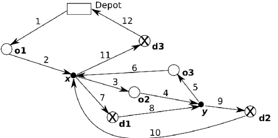
The following figure 1 provides us with a visualization of a valid tour = {(Depot, o1, 0), (o1, x, 1),
(x, o2, 0), (o2, y, 2), (y, o3, 0), (o3, x, 3), (x, d1, 1), (d1, y, 0), (y, d2, 2), (d2, 0, x), (x, d3, 3), (d3, Depot,
0)}.
Figure 1: Visualizing a valid tour .
All these definitions allow us to formally set our APSCP (Asymmetric Pre-emptive Stacker Crane Problem) Problem as follows:
{Given the node set X and the Shortest Path Distance Matrix DIST, compute a valid tour with minimal cost}.
III. Some Structural Results
.
We are now going to state and prove some results which will be the basis for the design of the heuristics which will be described in Section IV.
III. 1. A Theorem.
Let some valid tour. For any labelled link r = (x, o(k), 0) in , we denote by ( , r) the unique labelled link (d(k), y, 0) which is also in . By the same way, if x is some node in XR, such that a
triple a labelled link r = (y, x, k), k ≥ 1, is in , then we also denote by ( , r) the unique triple r’ = (x, z, k) which exists in G and which is such that:
- Rank( , r’) > Rank( , r);
- Rank( , r’) is minimal with this property.
We say that two Labelled links r and r’ in are overlapping if we have: Rank( , ( , r’)) > Rank( , ( , r)) > Rank( , r’) > Rank( , r). Then we may state:
Theorem 1.
Let be some optimal tour for the APSCP Problem, which we suppose chosen in such a way that: - (A): Length( ) is the smallest possible;
- (B): the number of labelled links r in which are such that Label(r) ≠ 0 is the smallest possible, (A) being supposed to be satisfied;
Then, the following assertions must be true:
- (S1): does not contain two occurrences of the same labelled link r = (x, y, k), with k ≠ 0; - (S2): does not contain two consecutive labelled links r and r’ such that Label(r) = Label(r’); - (S3): does not contain two overlapping labelled links r and r’;
- (S4): does not contain two labelled links r and r’ such that End(r) = End(r’). Proof.
We assume that is given, which is an optimal solution of APSCP and which is such that (A) and (B) are true.
Part (S1).
If r = (x, y, k), k > 0 appears twice in , with respectively rank s and s’, then x and y are both reload nodes, and we may replace, in any labelled link r” which is such that:
- s ≤ Rank( , r”) < s’; - Label( r”) = k;
the label value Label(r”) by 0. While doing it, we keep on with a valid tour which is an optimal solution of APSCP and we get a contradiction on the (B) hypothesis.
Part (S2).
If r = (x, y, k) and r’ = (y, z, k) were two consecutive labelled links of such that Label(r) = Label(r’), then we would be able to remove both r and r’ from , and replace them by a unique labelled link (x, z, k). While doing this, we would also keep, because of the Triangle property on the DIST matrix, an optimal solution of APSCP, and this solution would contradict the (A) hypothesis.
Let us suppose that there exists two labelled links r = (y, x, k) and r’ = (y’, x’, k’) which are overlapping in . We may choose them in such a way that Rank( , ( , r’)) – Rank( , r) is the
smallest possible. (E1)
Because of (E1), we see that x and x’ must be reload nodes: if, for instance, x were an origin node o(h), then we would have k’ ≠ h and there would exist an labelled link r” such that:
- Label(r”) = h;
- Rank(G, r) < Rank(G, r”) < Rank(G, r’) < Rank(G, ( , r”)) < Rank(G, ( , r)) < Rank(G, ( , r’)).
Then we might deduce a new overlapping pair (r”, r’) which would induce a contradiction on the minimality assumption (E1). By the same way, we may check that x’ cannot be an origin node o(h). Thus x and x’ are both reloads nodes, and we clearly have: k ≠ k’ ≠ 0.
It comes that we may write:
- r = (y, x, k), r’ = (y’, x’, k’) ; - ( , r) = (x, z, k), ( , r’) = (x’, z’, k’). So, we set : - 1 = I( , First( ), r) ; - 2 = I( , Succ( ,r), r’) ; - 3 = I( , Succ( ,r’), Pred( , ( , r))) ; - 4 = I( , ( , r), Pred( , ( , r’))) ; - 5 = I( , ( , r’), Last( )),a
and we replace by the concatenation Aux = 1 4 3 2 5 . Of course, the lengths
of and are Aux equal, as well as their respective costs. So we state: Lemma 1.
Aux defined above is a valid tour.
Proof-Lemma.
We only need to check that switching 2, 3 and 4 does not break any sequence (k), or, in other
words, that for any k ≠ 0, we have (k) = Aux(k). If the converse were true, we would be able to find
k” ≠ k’, k, k” ≠ 0, as well as two labelled links r” and ( , r”), with label k” or with the ending node of r” equal to o(k”), such that one of the three following relations would be true:
- r” 2 and ( , r”) 3; (E2);
- r” 2 and ( , r”) 4; (E3);
- r” 3 and ( , r”) 4; (E4);
In case (E2) or (E3) were true, r” and r’ would be overlapping, and would contradict the (E1) hypothesis, related to the minimality of Rank( , ( , r’)) – Rank( , r)
In case (E4) were true, r and r” would be overlapping, and would contradict the (E1) hypothesis, related to the minimality of Rank( , ( , r’)) – Rank( , r).
In any case, we become able to conclude. END-LEMMA.
The above lemma allows us to conclude the proof of (S3) by noticing that r and ( , r) become consecutive in the valid tour Aux, which implies (proof of statement (S2)) that r and ( , r) may be
replaced in Aux by a unique labelled link (y, z, k) in such a way that Cost( Aux) does not increase and
that Length( Aux) decreases, inducing a contradiction on the (A) hypothesis.
Part (S4).
Let us suppose that contains two labelled links r and r’ such that End(r) = End(r’) and such that Rank( , r) < Rank( , r’). Since the starting node x of r cannot be in {Depot} XD, it must be a
reload node in XR which is used twice as a reload node. So, r, ( , r) and r’ and ( , r’) may be
written:
- r = (y, x, k), k ≠ 0; - r’ = (y’, x, k’), k’ ≠ 0, k; - ( , r) = (x, z, k);
- ( , r’) = (x, z’, k’). Because of (S3) we must have:
- Rank( , r) < Rank( , ( , r)) < Rank( , r’) < Rank( , ( , r’)) (E5) or
- Rank( , r) < Rank( , r’) < Rank( , ( , r’)) < Rank( , ( , r)). (E6) Let us first suppose that (E5) holds. Then we set:
- 1 = I( , First( ), r) ;
- 2 = I( , Succ( ,r), Pred( , ( , r))) ;
- 3 = I( , ( , r), r’) ;
- 4 = I( ,Succ( ,r’), Pred( , ( , r’))) ;
- 5 = I( , ( , r’), Last( )),
and we replace by the concatenation Aux = 1 3 2 4 5 . Of course, the lengths
of and are Aux equal, as well as their respective costs, and we proceed as in the proof of (S3) in
order to prove that Aux must be a valid tour. But we also notice, as in the proof of (S3), that Aux can
be shortened by replacing the consecutive labelled links r and r* by a unique labelled link (y, z, k), in such a way that Cost( Aux) does not increase and that Length( Aux) decreases, inducing a contradiction
on the (A) hypothesis.
We apply exactly the same kind of reasoning in case (E6) holds. END-THEOREM. III. 2. A Tree Representation of the APSCP Problem.
Theorem 1 leads us to introduce the following definition:
Strongly Valid Tour: a valid tour is a strongly valid tour if it satisfies the (S1)…(S4) properties which are listed into the statement of Theorem 1.
The following figure 2 shows us how the valid tour of Figure 1 may be turned into a strongly valid tour whose cost ’ is no more than the cost of :
Figure 2: A derivation of the valid tour of figure 1 into a strongly valid tour ’.
Clearly, solving the APSCP Problem means finding a strongly valid tour with minimal cost value. Now, we are going to see that any strongly valid tour may be represented as some kind of tree, and this will provide us with the basis (section IV) for the algorithms which we are going to design in order to deal with APSCP.
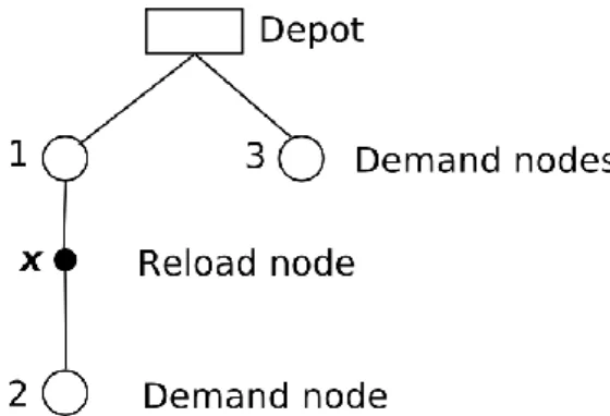
Bipartite Ordered Trees: we say that a tree T is a bipartite ordered tree if:
its nodes can be split into two classes A and B in such way that nodes in class A have their sons in class B and conversely;
for every node x in T which is not a terminal node (leaf) the son set (T, x) associated with x is linearly ordered: thus (T, x) is described as a sequence.
We say that a bipartite ordered tree T is consistent from the APSCP instance defined by the demand set K and by the node set X if:
- the nodes in T can be identified with the demands k K (we shall then talk about demand nodes) or with nodes in {Depot} XR, (and then we talk about reload nodes) and any possible demand
node k K appears in T, while only some of nodes of {Depot} XR appear in T: those nodes in
{Depot} XR define the active reload node set ACTIVE(T) of T; (S5)
- The root of T is the Depot node and the terminal nodes (leafs) of T must belong to the demand
node set; (S6)
- For any demand node k, its linearly ordered son set RELOAD(T, k) in T is made with active reload nodes and its father FATHER(T, k) is in ACTIVE(T); (S7) - For any reload node x, its linearly ordered son set DEMAND(T, x) in T is made with demand
nodes and its father FATHER(T, x) is in K. (S8)
For such a bipartite ordered tree T, we may define a cost value Tree-Cost as follows: - for any demand node k K: we set:
If k is not a terminal node then
Cost-Demand(T, k) = DIST(o(k), First(Reload(T,k))) + DIST(Last(Reload(T, k)), d(k))
+ x Reload(T, k), x ≠ Last(Reload(T,k)) DIST(x, Succ(Reload(T, k), x)))
else Cost-Demand(T, k) = DIST(o(k), d(k)) - for any reload node x {Depot} XR, we set:
Cost-Reload(T, k) =
DIST(x, o(First(Demand(T,x)))) + DIST(d(Last(Demand(T, x))), x) + k Demand(T, x), k ≠ Last(Demand(T,x)) DIST(d(k), o(Succ(Reload(T, x), k)));
- Tree-Cost(T) = Cost( ) = k K Cost-Demand(T, k) + x ACTIVE(T) Cost-Reload(T, x).
Theorem 2 : There is a one-to-one correspondence Tree between the strongly valid tours and the bipartite ordered tour which are consistent with X and K, which is such that, for any strongly valid tour , we have: Tree-Cost(Tree( )) = Cost( ).
Proof.
We first consider a strongly valid tour and perform the following construction, which make us get Tree( ) from :
- ACTIVE(T( )) is defined as the set of the nodes of {Depot} XR which appear in some
labelled link of , and which are then said to be active reload nodes for ;
- For any demand node k K, the son set Reload(T( ), k) is made with the reload nodes which appear in some labelled link of (k), ordered according to their appearance order in (k); - For any active reload node x in {Depot} XR, we denote by (x) = (x, y, 0) and by (x) = (z,
x, 0) the two labelled links with label 0 which involve x in and which are such that: Rank( , (x)) < Rank( , (x)). Then we define the son set Demand(T( ), x) by setting that a demand k K is a son of x if the unique labelled link r(k) = (o(k), t, k) which appears in is such that:
Rank( , (x)) < Rank( , r(k)) < Rank( , (x))
there exists no reload node y such that Rank( , (x)) < Rank( , (y)) < Rank( , r(k)) < Rank( , (y)) < Rank( , (x)).
Figure 3: The bipartite tree Tree( ’) which derives from the strongly valid tout ’ of Figure 2.
Then it comes next that checking that the so defined Tree correspondence is as it is claimed in the statement of Theorem 2 is purely routine. END-THEOREM.
We deduce:
Corollary 1: Solving a APSCP instance (X, DIST, K) means finding a bipartite ordered tree T consistent with (X and K) such that Tree-Cost(T) is the smallest possible.
The interest of this last statement is clearly that it provides us with a bipartite tree formulation of the APSCP problem which is far less constrained that the original one.
III.3. A related Integer Linear Programming formulation of APSCP
.
This ILP formulation is going to allow us to compare, in the case of small instances, the results obtained through the heuristic methods which will be described in Section IV with exact results. In order to get it, we first need to proceed to the following construction:
- An auxiliary network G = (X*, E).
We first consider a copy X*R of the reload node set XR and a copy Depot* of the Depot node,
and we set: X* = X X*R {Depot*};
For any node x in XR, we denote by x* its copy in X*R. Also, for any origin node x = o(k) in
XO, we denote by x* the related node d(k).
Then we define, on the node set X*, the arc set E as follows:
- E = {(Depot, x), x XO} {(x, Depot*), x XD} {(o(k), d(k)), k K}
{(d(k’), o(k)), k ≠ k’ K}
{(x, y), (y, x), x XO, y XR} {(x, y) (y, x), x X*R, y XD}
{(x, y), x X*R, y XR}.
- every arc e in E is then provided with a length DIST*(e) which derives from the DIST distance matrix in a natural way.
Let us recall that a path of a such a network G is a node sequence such that, for any node x in , the pair (x, Succ( , x)) defines an arc of E. One easily checks that any strongly valid tour can be turned into a path * of the network G, in such a way that:
- (S9): * starts from Depot and ends into Depot* and * is an elementary path, i.e, its visits any node at most once;
- (S10): for every k in K, * visits o(k) and d(k), according to this order and for every x in XR,
* visits x if and only if it visits x*, and, in case it does it, it does it according to this order; - (S11): for any pair x, y, x ≠ y, in XR XO the following implication is true:
Rank( *, x) < Rank( *, y) and Rank( *, y) < Rank( *, x*) =>
Rank( *, y*) < Rank( *, x*).
This condition is called the non overlapping condition.
- (S12): Cost( ) = x x ≠ Depot* DIST*(x, Succ( *, x)) = Length of * for the DIST* length
function.
A path of the network G which satisfies (S9)…(S12) above will be said to be a strongly valid path. Theorem 3.
For any strongly valid path , there exists a strongly valid tour such that * = . Proof.
Let us first describe in an accurate the way is going to derives from . It will occur through the following RECONSTRUCT procedure:
RECONSTRUCT Procedure x <- Depot; <- Nil;
While x <> Depot* do y <- Succ( , x);
If y may be written y = z*, with z {Depot} XR, then we set (y) = z,
else we set (y) = y;
If (multi-case branching instruction) 1. x = Depot then <- (x, y, 0)* ; 2. x = o(k), k K then <- (x, y, k)* ; 3. x XR then <- (x, (y), 0)* ;
4. x XD then <- (x, (y), 0)* ;
5. x X*R then <- (x, y, k)* , where k ≠ 0 is such that the labelled link (Pred( ,
(x)), (x), k) is already in ; (I1)
The instruction (I1) works here because of (S10) above, and because an arc of G which arrives on (x) must come from an origin node o(k) or from a node z in X*R. In this last case, a simple induction
reasoning makes appear the fact that k is different from 0.
We get our result while proceeding by induction on the length (the number of nodes) of . In case involves no node in XR, then the results come in a trivial way. Else, we consider x0 XR which is the
first node of XR which appears in . We notice that Pred( , x0) must be some node o(k), k K. Thus
the arc (Pred( , x0), Succ( ,x0*)) belongs to the arc set E, and the removal of the subpath I( , x0, x0*)
from provides us with an other path 1 of the graph G. Let us set:
K1 = { k K such that o(k) and d(k) are nodes of 1};
K2 = { k K such that o(k) and d(k) are nodes of 2 = I( , x0, x0*)};
K1 and K2 define a partition of K, and one sees that 2 can be viewed as a strongly valid path, if we
restrict ourselves to K2 as a demand set and if we consider that x0 and x0* play the role of Depot and
Depot*. Thus it comes from the induction hypothesis that it may be written, under this restriction, according to the form 2 = *2. By the same way, 1 is also a strongly valid path if we restrict the
demand node set to K1, and it comes from the induction hypothesis that it may be written, under this
restriction, according to the form 1 = *1. We only need to insert 2 between Pred( , x0), x0, k) and
(x0, Succ( , x0*), k) in 1, in order to get such that = *. END-THEOREM.
Corollary 2: Solving a APSCP instance (X, DIST, K) means finding a strongly valid path with minimal length (for the DIST* length function) value in the network G.
This corollary allows us to set an Integer Linear Programming model as follows:
This model involves a {0, 1} vector flow z = (ze, e E), a Rank integral vector R = (Rx, x
X), as well as a positional {0, 1}vector t, which is indexed on the pairs (x, y), x ≠ y, x, y XR
XO , with the following semantics:
- for any node x in , Rx will provide us with the rank of x in ;
- for any pair (x, y), x ≠ y, x, y XR XO :
tx,y = 1 iff Rank( , y) < Rank( , x*);
tx,y = 0 iff Rank( , x*) < Rank( , y);
Then the translation of (S9)…(S12) into Integer Linear Programming constraints provides us with the following linear integer program:
APSCP Integer Linear Programming Formulation.
Unknown vectors.
z = (ze, e E), with values in {0,1}; R = (Rx, x X) Integral and ≥0;
t = (tx,y, x ≠ y, x, y XR XO) with values in {0,1}. Performance Criterion.
Minimize e E DIST*(e).ze (translation of (S12)) Constraints.
- z is a flow vector, which satisfies the usual Kirshoff law in any node but in Depot and Depot*; - the inflow induced by z in Depot (Depot*) is equal to 0 (1), while the related outflow is equal
to 1 (0); (translation of (S9))
- in any node of XD XO, the inflow induced by z is equal to 1; (translation of (S10))
- in any node of XR X*R, the inflow induced by z is at most equal to 1, and the inflow value
in x is equal to the inflow value in x*; (translation of (S10) and (S9)) - for any k in K, we have Ro(k) ≤ Rd(k) – 1; (translation of (S10))
- for any x in XR, we have Rx ≤ Rx* – 1; (translation of (S10))
- for any arc e = (x,y) in E, we have ze + (Rx + 1 - Ry )/Card(X*) ≤1; (translation of the
implication ze = 1 -> (Rx + 1 - Ry) ≤0)
- for any pair (x, y), x ≠ y, x, y XR XO : (translation of the non overlapping condition)
tx,y + (Ry + 1 - Rx* )/Card(X*) ≤1 ;
tx,y + (Ry - 1 - Rx* )/Card(X*) 0 ;
tx,y + (Ry* + 1 - Rx* )/Card(X*) ≤1.
Corollary 2: Solving a APSCP instance (X, DIST, K) means solving the above Integer Linear Programming model.
IV. Tree Based Heuristics for the APSCP Problem
.
The algorithms which we are going to describe here, and which will be tested in the next Section, derive in a straightforward way from the tree representation of the APSCP Problem which we got in Section III.2. These algorithms are very simple greedy insertion algorithms and descent algorithms, based upon the use of 2 classes of operators:
Insertion Operators: these operators act on some bipartite ordered tree T consistent with the node set X and with a subset K’ of the demand set K, and insert some demand k K – K’ in T. We use two operators:
INSERT-SIMPLE: its parameters are some active reload node x in {Depot} XR, and some
cut (l1, l2) of the sequence DEMANDE(T, x) = l1 l2. It acts by inserting the segment {k} into
this cut: DEMANDE(T, x) <- l1 {k} l2 .
INSERT-with-RELOAD: its parameters are some demand node k’ in K’, a cut c = (l1, l2) of the
- inserting the segment {x} into the cut c: RELOAD(T, x) <- l1 {x} l2;
- by making x be active and setting: DEMAND(T, x) <- {k}; RELOAD(T, k) <- Nil.
Local Transformation Operators: these operators act through side effect on some bipartite ordered tree T consistent with X and K, and they modify T. We use 6 operators:
- MOVE-RELOAD: its parameters are some active reload node x and some non active reload node y. It replaces x by y in T.
- MOVE-RELOADS: its parameters are two different demand nodes k and k’, a segment l of RELOAD(T, k) and a cut c = (l1, l2) of RELOAD(T, k’). It removes l from RELOAD(T, k)
and it inserts it into the cut c. Its precondition is that k does not dominate k’ in the tree T, i.e, that k cannot be obtained from k’ through a succession of applications of the FATHER operator.
- MOVE-RELOADS1: its parameters are some demand node k, some segment l of RELOAD(T, k) which induces a decomposition RELOAD(T, k) = l3 l l4, and a cut c = (l1,
l2) of l3 l4. It first remove l and next insert it into the cut c: RELOAD(T, k’) <- l1 l l2.
- MOVE-DEMANDS: its parameters are two different active reload nodes x and y, a segment l of DEMAND(T, x), and a cut c = (l1, l2) of DEMAND(T, x’). It removes l from DEMAND(T,
x) and it inserts it into the cut c. In case l1 = l2 = Nil, it remove the reload node x from T,
which becomes non active. Its precondition is that x does not dominate y in the tree T. - MOVE-DEMAND1: its parameters are some reload node x, some segment l of DEMAND(T,
x) which induces a decomposition DEMAND(T, x) = l3 l l4, and a cut c = (l1, l2) of l3
l4. It first remove l and next insert it and it into the cut c: DEMAND(T, x) <- l1 l l2 .
- MOVE-DEMANDS-RELOAD: its parameters are an active reload node x, a non active reload node y, a demand node k, a segment l of DEMAND(T, x) and a cut c = (l1, l2) of RELOAD(T,
k). It first turns y into an active reload node, next removes l from DEMAND(T, x) and inserts it into DEMAND(T, y), and ends in inserting the segment {y}into the cut c. In case l = DEMAND(T, x), it turns x into a non active reload node. Its precondition is that k is dominated by not demand node k’ in l.
Then we can propose a first insertion greedy algorithm for dealing with APSCP: Algorithm APSCP-INSERTION:
Randomly define a linear ordering on the elements of K; T = {the tree reduced to the root node Depot};
For k K, K being scanned according to the linear order do
Compute the insertion operator I (among INSERT-SIMPLE and INSERT-with-RELOAD) and the related parameter u (u = (x, (l1, l2)) in case I = INSERT-SIMPLE, u =
(k’, (l1, l2), x) in case I = INSERT-with-RELOAD), such that the insertion of k through
I(u) induces the smallest possible increase of Tree-Cost(T); Apply I(u) to T;
Filtering the search for the good value of the parameter u.
In case I = INSERT-SIMPLE, the related optimal value of u can be obtained in a very fast way through exhaustive scanning of the sequences DEMAND(T, x) for all the active reload nodes x. In case I = INSERT-with-RELOAD, one must deal with the search for the new reload node x, which may be time consuming in case XR is large. In order to avoid spending too much time while trying all the
possible reload nodes x, we try to identify in a fast way those nodes which are likely to provide us with an efficient insertion by proceeding as follows:
- for every node x in XR, we keep in memory a set N(x) of neighbours of x, that means of nodes
y which are such that DIST(x, y) ≤ R, where R is some threshold which is chosen in such a way that the induced neighbour graph be connected, and that the cardinality of any set N(x) remains small enough.
- by the same way, we keep in memory, for every pair of reload nodes (x, y), what we call the middle of x and y, that means some node z = MID(x, y) which is such that the difference between DIST(x, z) + DIST(z, y) – DIST(x, y) remains small, both quantities DIST(x, z) and DIST(y, z) being close to each other;
- if we denote by y the last reload node in l1 and by z the first reload node in l2, then we see that
we should try to select x in such a way that DIST(y, x) + DIST(x, o(k)) + DIST(d(k), x) + DIST(x, z) be the smallest possible. Instead of trying all the possible nodes of XR we do it by
selecting t = MID(MID(y, o(k)), MID(d(k), z)) and by trying all the nodes x in N(t).
Of course, the algorithm APSCP-INSERTION may be used inside a Monte-Carlo Scheme as follows:
Parameter :
For i = 1 to run the APSCP-INSERTION Procedure; Keep the best result.
This greedy insertion algorithm may now used in order to initialize the following APSCP-DESCENT descent algorithm:
Algorithm APSCP-DESCENT:
Initialize the tree T through APSCP-INSERTION; Initialize the filtering threshold value H;
(1): Search (in a filtered way) parameter values x, y for the MOVE-RELOAD operator in such a way that applying MOVE-RELOAD(x, y) to T improves the Tree-Cost quantity; If Success then Go To (1);
(2): Search (in a filtered way) parameter values k, k’, l, c for the MOVE-RELOADS operator in such a way that applying MOVE-RELOADS(k, k’, l, c) to T improves the Tree-Cost quantity; If Success then Go To (1);
(3): Search (in a filtered way) parameter values k, l, c for the MOVE-RELOADS1 operator in such a way that applying MOVE-RELOADS1(k, l, c) to T improves the Tree-Cost quantity; If Success then Go To (1);
(4): Search (in a filtered way) parameter values x, y, l, c for the MOVE-DEMANDS operator in such a way that applying MOVE-DEMANDS(x, y, l, c) to T improves the Tree-Cost quantity; If Success then Go To (1);
(5): Search (in a filtered way) parameter values x, l, c for the MOVE-DEMANDS1 operator in such a way that applying MOVE-DEMANDS1(x, l, c) to T improves the Tree-Cost quantity; If Success then Go To (1);
(6): Search (in a filtered way) parameter values x, y, k, l, c for the MOVE-DEMANDS-RELOAD operator in such a way that applying MOVE-DEMANDS-MOVE-DEMANDS-RELOAD(x, y, k, l, c) to T improves the Tree-Cost quantity; If Success then Go To (1);
(7): If H is small enough then Stop else set H = H/2 and go to (1). Filtering the search for the good value of the parameter vectors.
In the case of the (1) above instruction, the active nodes x are scanned in an exhaustive way, but the search for the y value is restricted to the neighbourhood set N(x).
In the case of the instruction (2) and (3), the threshold value H is involved as followed:
- the segment l is tried only if the decomposition RELOAD(T, k) = l3 l l4 is such that
DIST(Last(l3), First (l)) and DIST (Last(l), First(l4 )) ≥ H;
- the cut c = (l1, l2) is tried only if DIST(Last(l1), First (l2)) ≥ H.
- the segment l is tried only if the decomposition DEMAND(T, x) = l3 l l4 is such that
DIST(d(Last(l3)), o(First (l))) and DIST (d(Last(l)), o(First(l4 ))) ≥ H;
- the cut c = (l1, l2) is tried only if DIST(d(Last(l1)), o(First (l2))) ≥ H.
In the case of the (6) instruction, the threshold value H is involved as in (4) and (5), and the search for y is performed, once x, k, l, c = (l1, l2) have been determined inside the neighbour set N(t) of t =
MID(MID(Last(l1), o(First(l))), MID(d(last(l)), First(l2))).
Remark: of course, it would be possible to improve the performance of the APSCP-DESCENT algorithm by casting it into a scheme like the Simulated Annealing scheme or the Tabu List scheme. But it is not really the purpose of the paper: as we shall see in Section V, our tree representation of the APSCP problem, together with the operators which we just described above, are sufficiently powerful to provide us, under small computing costs, with very good solutions for our APSCP problem.
V. Experiments
.
We have been performing experiments, on PC IntelXeonwith 1.86 GHz, 3.25 Go Ram, while using a Visual Studio C++ compiler, and while focusing on several points:
- the ability of APSCP-INSERTION and APSCP-DESCENT to get solutions close to the optimal theoretical solutions;
- the running time of those algorithms;
- the characteristics of the solutions: number of reload nodes which appear in the solution, improvement of the Cost-Tree value induced by pre-emption;
- the impact of the different local transformation operators on the behaviour of the algorithms. In order to do this, we performed several tests, while using node sets X and distance matrices DIST proposed by the TSPLIB libraries, and by selecting origin/destination pairs (o(k), d(k), k K) in a random way inside the set X. We dealt with instances which involves from 20 to 300 nodes, and from 10 to 100 origin destination pairs, and, in case of small instances, got exact results through the use of the LIP formulation of Section III.3, augmented with cutting planes techniques (see [25, 26]).
Our first experiment is related to the procedure INSERTION: we run the APSCP-INSERTION Monte-Carlo scheme with = 100, and we keep memory, for every test with name INST, of the followingquantities:
REF: Optimal theoretical Tree-cost value;
MIN (MAX): Minimal (Maximal) Tree-cost value obtained through iterations of APSCP-INSERTION; MEAN: Maximal (worse) Tree-cost value obtained;
EGI: Gap (in %) between REF and the global solution produced by the APSCP-INSERTION Monte Carlo scheme (MIN value).
REL: Mean number of reload nodes involved in a solution produced by APSCP-INSERTION; DE/REL: Mean number of demands related to every reload node x (length of the list DEMAND(x)), for x different from Depot;
CPU: CPU Mean Time (in milliseconds) for any iteration of APSCP-GREEDY-INSERTION.
The results which we get may be summarized as follows:
Table 1: Tests performed on 10 instances which we got from the gr24 instance with 49 nodes of the
TSPLIB library by randomly sorting 12 demands, and no reload nodes which is not the depot node, the copy of an origin node o(k) or the copy of a destination node d(k), k 1..12.
Gr24_v01 24654 25023 27883 26391 1.5 0.06 2.83 < 15 Gr24_v02 21395 21424 23654 22371 0.136 0.43 1.60 < 15 Gr24_v03 22834 23363 26825 24760 2.32 0.36 2.51 < 15 Gr24_v04 23255 23444 25513 24140 0.813 0.41 2.47 < 15 Gr24_v04 23993 23993 27373 25261 0 0.31 2.03 < 15 Gr24_v06 23233 23233 25584 24427 0 0.54 1.71 < 15 Gr24_v07 20224 20283 22594 20906 0.292 0.11 1.72 < 15 Gr24_v08 20865 21124 23334 21873 1.24 0.61 1.13 15 Gr24_v09 23054 23073 25684 24014 0.0824 0.43 3 < 15 Gr24_v10 26704 26963 29843 28303 0.97 0.16 4.4 15
Table 2: Tests performed on 10 instances which we got from the hk48 instance with 97 nodes of the
TSPLIB library by randomly sorting 24 demands, and no reload nodes which is not the depot node, the copy of an origin node o(k) or the copy of a destination node d(k), k 1..24.
INST REF MIN MAX MEAN EGI REL DE/REL CPU Hk48_v01 358048 375447 405299 387605 4.86 0.97 1.67 < 15 Hk48_v02 280579 291800 325548 306673 4 1.44 1.39 < 15 Hk48_v03 318959 325027 351678 338017 1.9 0.95 3.25 < 15 Hk48_v04 315118 322908 347647 336123 2.47 0.53 2.46 15 Hk48_v04 320578 327709 360167 340639 2.22 0.27 2.80 15 Hk48_v06 306000 318838 351007 334372 4.2 0.59 4.42 < 15 Hk48_v07 314127 330528 370107 347588 5.22 0.52 3.04 16 Hk48_v08 342390 350960 381719 366652 2.5 0.53 4.57 16 Hk48_v09 337327 343127 370387 355734 1.72 0.54 3.24 15 Hk48_v10 330119 339509 373190 355208 2.84 0.73 1.61 16
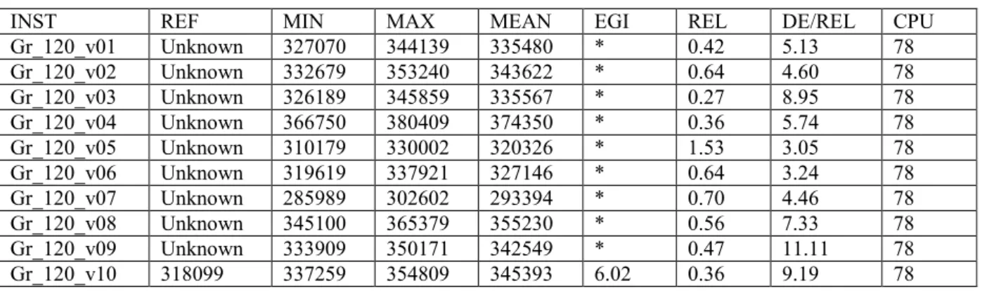
Table 3: Tests performed on 10 instances which we got from the gr120 instance with 241 nodes of the
TSPLIB library by randomly sorting 60 demands, and no reload nodes which is not the depot node, the copy of an origin node o(k) or the copy of a destination node d(k), k 1..60.
INST REF MIN MAX MEAN EGI REL DE/REL CPU Gr_120_v01 Unknown 327070 344139 335480 * 0.42 5.13 78 Gr_120_v02 Unknown 332679 353240 343622 * 0.64 4.60 78 Gr_120_v03 Unknown 326189 345859 335567 * 0.27 8.95 78 Gr_120_v04 Unknown 366750 380409 374350 * 0.36 5.74 78 Gr_120_v05 Unknown 310179 330002 320326 * 1.53 3.05 78 Gr_120_v06 Unknown 319619 337921 327146 * 0.64 3.24 78 Gr_120_v07 Unknown 285989 302602 293394 * 0.70 4.46 78 Gr_120_v08 Unknown 345100 365379 355230 * 0.56 7.33 78 Gr_120_v09 Unknown 333909 350171 342549 * 0.47 11.11 78 Gr_120_v10 318099 337259 354809 345393 6.02 0.36 9.19 78
Table 4: Tests performed on 10 instances RELn, , which we built in such a way that:
- the related instance involves n nodes, p = (n/2 -1)/3 – 1 reload nodes, (n – p – 1)/2 demands; - its optimal value is the sum k K DIST(o(k), d(k)), and that the related optimal solution
involves all the reload nodes.
REL31 11843 13045 17088 14665 10.1 0.11 0.68 < 15 REL55 17464 19554 23322 21841 12.0 0.35 2.40 16 REL79 21053 24235 28386 26194 15.1 0.54 2.92 31 REL91 22323 26321 29924 27658 17.9 0.54 2.85 47 REL115 24142 28117 31813 30000 16.5 0.91 4.50 78 REL163 26036 30734 35302 32966 18.0 1.76 5.61 141 REL187 26494 32077 36486 34092 21.1 2.87 4.83 187 REL211 26775 32830 36434 34655 22.6 3.39 4.83 250 REL259 27042 33773 38796 35654 24.9 5.92 4.70 375 REL283 27098 33664 37496 36035 24.2 6.86 5.17 453
Comments: We see that the results which we get through application of a combination of a greedy scheme and a Monte-Carlo diversification scheme are most often rather goods, in the sense that its allows us to get in a fast way solutions which are not too far from the best theoretical ones. Still, we also notice that our greedy scheme is in trouble when it comes to pre-emption handling, that means when it comes to creating reload nodes. Thus, the results which derive from the application of APSCP-INSERTION get worse as soon as there is an increase of the gap between the optimal pre-emptive optimal value and the non pre-pre-emptive one.
Our second experiment is related to APSCP-DESCENT. We run APSCP-DESCENT from a solution provided by only 1 application of APSCP-INSERTION, and we keep memory, for every test with name INST, of the following quantities:
REF: Optimal theoretical value;
VAL: The cost value obtained after application of APSCP-DESCENT;
EGI: Gap (in %) between REF and the solution produced by APSCP-INSERTION; ED: Gap between REF and the solution produced by APSCP-DESCENT;
ETDS: Part of the gap between EGI and ED which is induced by the operators MOVE-DEMANDS and MOVE-MOVE-DEMANDS1 and MOVE-DEMAND-with-RELOAD;
REL: Number of reloads involved in the solution produced by APSCP-DESCENT;
TNB: Number of times a local transformation operator is effectively applied inside the APSCP-DESCENT process;
CPU: Cpu Running Time (in milliseconds).
The results which we get may be summarized as follows:
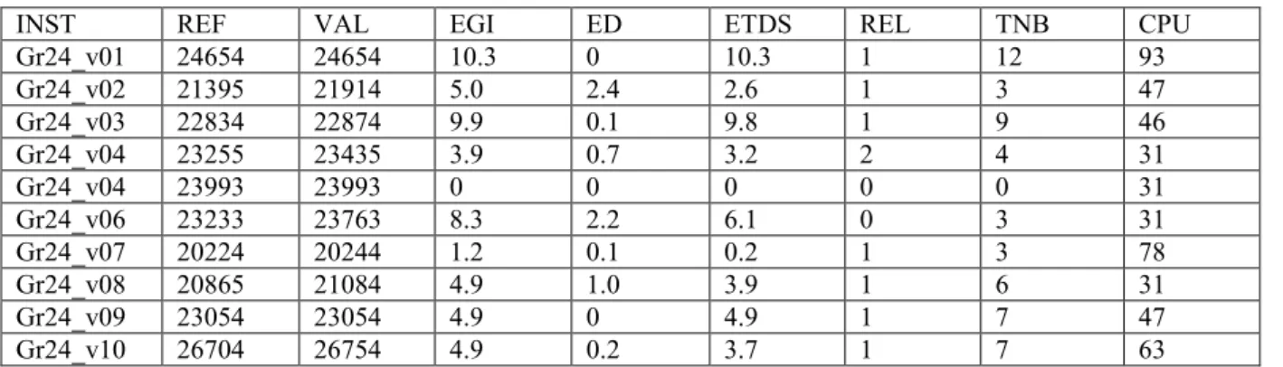
Table 5: Tests performed on 10 instances which we got from the gr24 instance with 49 nodes of the
TSPLIB library by randomly sorting 12 demands, and no reload nodes which is not the depot node, the copy of an origin node o(k) or the copy of a destination node d(k), k 1..12.
INST REF VAL EGI ED ETDS REL TNB CPU Gr24_v01 24654 24654 10.3 0 10.3 1 12 93 Gr24_v02 21395 21914 5.0 2.4 2.6 1 3 47 Gr24_v03 22834 22874 9.9 0.1 9.8 1 9 46 Gr24_v04 23255 23435 3.9 0.7 3.2 2 4 31 Gr24_v04 23993 23993 0 0 0 0 0 31 Gr24_v06 23233 23763 8.3 2.2 6.1 0 3 31 Gr24_v07 20224 20244 1.2 0.1 0.2 1 3 78 Gr24_v08 20865 21084 4.9 1.0 3.9 1 6 31 Gr24_v09 23054 23054 4.9 0 4.9 1 7 47 Gr24_v10 26704 26754 4.9 0.2 3.7 1 7 63
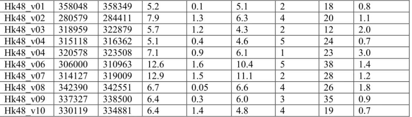
Table 6: Tests performed on 10 instances which we got from the hk48 instance with 97 nodes of the
TSPLIB library by randomly sorting 24 demands, and no reload nodes which is not the depot node, the copy of an origin node o(k) or the copy of a destination node d(k), k 1..24.
Hk48_v01 358048 358349 5.2 0.1 5.1 2 18 0.8 Hk48_v02 280579 284411 7.9 1.3 6.3 4 20 1.1 Hk48_v03 318959 322879 5.7 1.2 4.3 2 12 2.0 Hk48_v04 315118 316362 5.1 0.4 4.6 5 24 0.7 Hk48_v04 320578 323508 7.1 0.9 6.1 1 23 3.0 Hk48_v06 306000 310963 12.6 1.6 10.4 5 38 1.4 Hk48_v07 314127 319009 12.9 1.5 11.1 2 28 1.2 Hk48_v08 342390 342551 6.7 0.05 6.6 4 26 1.8 Hk48_v09 337327 338500 6.4 0.3 6.0 3 35 0.9 Hk48_v10 330119 334881 6.4 1.4 4.8 4 19 0.7
Table 7: Tests performed on 10 instances which we got from the gr120 instance with 241 nodes of the
TSPLIB library by randomly sorting 60 demands, and no reload nodes which is not the depot node, the copy of an origin node o(k) or the copy of a destination node d(k), k 1..60.
INST REF VAL EGI ED ETDS REL TNB CPU (s) Gr_120_v01 Unknown 313315 * * 5.2 6 89 130 Gr_120_v02 Unknown 318870 * * 8.9 1 116 189 Gr_120_v03 Unknown 314493 * * 6.2 4 96 125 Gr_120_v04 Unknown 360902 * * 3.5 3 107 145 Gr_120_v05 Unknown 293613 * * 9.8 4 99 125 Gr_120_v06 Unknown 303441 * * 7.7 2 90 80 Gr_120_v07 Unknown 265713 * * 6.4 4 84 86 Gr_120_v08 Unknown 330823 * * 6.9 4 77 94 Gr_120_v09 Unknown 314073 * * 8.5 4 105 70 Gr_120_v10 318099 318913 9.5 0.25 9.1 4 96 103
Table 8: Tests performed on 10 instances RELn, , which we built in such a way that:
- the related instance involves n nodes, p = (n/2 -1)/3 – 1 reload nodes, (n – p – 1)/2 demands; - its optimal value is the sum k K DIST(o(k), d(k)), and that the related optimal solution
involves all the reload nodes.
INST REF VAL EGI ED ETDS REL TNB CPU
REL31 11843 11953 16.7 0.9 15.8 4 10 0.04 REL55 17464 17583 27 0.7 36.3 8 28 0.34 REL79 21053 21053 29.9 0 29.9 12 56 1.5 REL91 22323 22605 20.8 1.2 19.6 14 46 2.9 REL115 24142 24225 28.4 0.34 28.4 18 78 8.4 REL163 26036 26279 19.3 0.93 18.3 26 79 25 REL187 26494 26626 26.6 0.49 26.2 30 112 39 REL211 26775 26851 33.1 0.28 30.1 34 134 78 REL259 27042 27067 37 0.09 36.9 42 162 232 REL283 27098 27211 33.1 0.4 32.4 46 202 328
Comments: We first notice that the gap between pre-emption and non pre-emption may greatly differ according to the way APSCP instances are generated. Though APSCP-DESCENT does not involve any of the classical control mechanisms which allow dealing with local optima (Simulated Annealing, Tabou Search…), we see that the operators which derive from our tree representation enable us to get very satisfactory results in a very short time.
VI. Conclusion
.
We have been dealing here with a pre-emptive demand routing problem with capacity constraints, and we showed how it was possible to turn it into a non constrained tree construction problem in such a
way that we could solve it in an efficient way through simple greedy and descent processes. It would be interesting to extend the approach which we presented here in a very specific context, and try to deduce efficient approaches for the handling of pre-emption in more general routing and scheduling problems.
VII. Bibliography
.
[1] S. Anily, M. Gendreau, and G. Laporte. The preemptive swapping problem on a tree. Technical report, Les Cahiers du GERAD, G-2005-69, 2006.
[2] S. Anily and R. Hassin. The swapping problem. Networks, 22(4):419–433, 1992.
[3] N. Ascheuer, L. Escudero, M. Grötschel, and M. Stoer. A cutting plane approach to the sequential ordering problem (with applications to job scheduling in manufacturing). SIAM Journal on Optimization, 3:25–42, 1993.
[4] N. Ascheuer, M. Jünger, and G. Reinelt. A Branch & Cut algorithm for the Asymmetric Traveling Salesman Problem with Precedence Constraints. Computational Optimization and Applications, 17:61–84, 2000.
[5] M.J. Atallah and S.R. Kosaraju. Efficient Solutions to Some Transportation Problems with Applications to Minimizing Robot Arm Travel. SIAM Journal on Computing, 17:849, 1988.
[6] E. Balas, M. Fischetti, and W. Pulleyblank. The precedence constrained asymmetric traveling salesman problem. Mathematical Programming, 68:241–265, 1995.
[7] G.Berbeglia, J.F.Cordeau, I.Gribkovskaia, and G.Laporte. Static pickup and delivery problems: a classification scheme and survey. TOP: An Official Journal of the Spanish Society of Statistics and Operations Research, 15(1):1–31, July 2007.
[8] C. Bordenave, M. Gendreau, and G. Laporte. A branch-and-cut algorithm for the preemptive swapping problem. Technical Report CIRRELT-2008-23, 2008.
[9] C. Bordenave, M. Gendreau, and G. Laporte. Heuristics for the mixed swapping problem. Technical Report CIRRELT-2008-24, 2008.
[10] S.Chen and S.Smith. Commonality and genetic algorithms. Technical Report CMU-RI-TR-96-27, Robotics Institute, Carnegie Mellon University, Pittsburgh, PA, December 1996.
[11] J.F. Cordeau, M. Iori, G. Laporte, and J.J. Salazar-González. A branch-and-cut algorithm for the pickup and delivery traveling salesman problem with LIFO loading. Submitted to publication, 2006. [12] J.F.Cordeau and G.Laporte. The dial-a-ride problem: models and algorithms. Annals of Operations Research, 153(1):29–46, 2007.
[13] C.E. Cortés, M Matamala, and C.Contardo. The Pickup and Delivery Problem with Transfers: Formulation and Solution Approaches. In VII French – Latin American Congress on Applied Mathematics. Springer, 2005.
[14] I.Dumitrescu. Polyhedral results for the pickup and delivery travelling salesman problem. Tech. Rep., CRT-2005-27, 2005.
[15] M.T.Fiala Timlin. Precedence constrained routing and helicopter scheduling. M. Sc. Thesis, Department of Combinatorics and Optimization University of Waterloo, 1989.
[16] M.T.Fiala Timlin and W.R.Pulleyblank. Precedence constrained routing and helicopter scheduling: heuristic design. Interfaces, 22:100–111, 1992.
[17] G.N. Frederickson and DJ Guan. Preemptive Ensemble Motion Planning on a Tree. SIAM Journal on Computing, 21:1130, 1992.
[18] G.N. Frederickson and D.J.Guan. Nonpreemptive ensemble motion planning on a tree. Journal of Algorithms, 15(1):29–60, 1993.
[19] G.N. Frederickson, M.S. Hecht, and C.E. Kim. Approximation Algorithms for Some Routing Problems. SIAM Journal on Computing, 7:178, 1978.
[20] L.M. Gambardella and M. Dorigo. An ant colony system hybridized with a new local search for the sequential ordering problem. INFORMS Journal on Computing, 12(3):237–255, 2000.
[21] L. Gouveia and P. Pesneau. On extended formulations for the precedence constrained asymmetric traveling salesman problem. Networks, 48(2):77–89, 2006.
[22] P.Healy and R.Moll. A new extension of local search applied to the Dial-A-Ride Problem. European Journal of Operational Research, 83(1):83–104, 1995.
[23] H.Hernández-Pérez and J.Salazar-González. The multicommodity one-to-one pickup-and-delivery traveling salesman problem. Submitted to European Journal of Operational Research, 2008. [24] B.Kalantari, A.V.Hill, and S.R.Arora. An algorithm for the traveling salesman problem with pickup and delivery customers. European Journal of Operational Research, 22:377–386, 1985. [25] H.L.M. Kerivin, M. Lacroix, and A. R. Mahjoub. Models for the single-vehicle preemptive pickup and delivery problem. Submitted to Journal of Combinatorial Optimization, 2007.
[26] H.L.M. Kerivin, M. Lacroix, and A.R. Mahjoub. The Eulerian closed walk with precedence path constraints problem. Technical Report LIMOS/RR-08-03 (also submitted for publication in SIAM Journal of Computing), 2007.
[27] S. Lin. Computer solutions to the traveling salesman problem. Bell System Technical Journal, 44:2245–2269, 1965.
[28] S. Lin and B. W. Kernighan. An effective heuristic algorithm for the traveling salesman problem. Operations Research, 21(2):498–516, 1973.
[29] J. Little, K. Murty, D. Sweeney, and C. Karel. An algorithm for the traveling salesman problem. Operations Research, 11(6):972–989, 1963.
[30] S. Mitrovic-Minic. Pickup and delivery problem with time windows: A survey. Technical Report SFU CMPT TR 1998-12, May 1998.
[31] S. Mitrovic-Minic and G. Laporte. The pickup and delivery problem with time windows and transshipment. INFOR, 44:217–227, 2006.
[32] R. Montemanni, D.H. Smith, and L.M. Gambardella. A heuristic manipulation technique for the sequential ordering problem. Computers & Operations Research, 35(12):3931–3944, 2008.
[33] P. Oertel. Routing with Reloads. Doktorarbeit, Universität zu Köln, 2000.
[34] S.N. Parragh, K.F. Doerner, and R.F. Hartl. A survey on pickup and delivery problems: Part II: Transportation between pickups and delivery locations. Journal für Betriebswirtschaft, 58(1):21–51, 2008.
[35] H. N. Psaraftis. A Dynamic Programming Solution to the Single-Vehicle Manyto-Many Immediate Request Dial-a-Ride Problem. Transportation Science, 14: 130–154, 1980.
[36] H.N. Psaraftis. k-interchange procedures for local search in a precedence constrained routing problem. European Journal of Operational Research, 13(4): 391–402, August 1983.
[37] J.Renaud, F. Boctor, and G.Laporte. Perturbation heuristics for the pickup and delivery traveling salesman problem. Computers & Operations Research, 29(9):1129–1141, 2002.
[38] J.Renaud, F. Boctor, and J.Ouenniche. A heuristic for the pickup and delivery traveling salesman problem. Comput. Oper. Res., 27(9):905–916, 2000.
[39] K. M. Ruland and E. Y. Rodin. The pickup and delivery problem: Faces and branch-and-cut algorithm. Computers and Mathematics with Applications, 33:1–13, 1997.
[40] M. W. P. Savelsberg and M. Sol. The general pickup and delivery problem. Transportation Science, 29(1):17–29, 1995.