Studying the ISM at ∼ 10 pc scale in NGC 7793 with MUSE -I. Data description and properties of the ionised gas

HAL Id: hal-02989839

https://hal.archives-ouvertes.fr/hal-02989839

Submitted on 5 Nov 2020

HAL is a multi-disciplinary open access

archive for the deposit and dissemination of

sci-entific research documents, whether they are

pub-lished or not. The documents may come from

teaching and research institutions in France or

abroad, or from public or private research centers.

L’archive ouverte pluridisciplinaire HAL, est

destinée au dépôt et à la diffusion de documents

scientifiques de niveau recherche, publiés ou non,

émanant des établissements d’enseignement et de

recherche français ou étrangers, des laboratoires

publics ou privés.

MUSE -I. Data description and properties of the ionised

gas

Lorenza Della Bruna, Angela Adamo, Arjan Bik, Michele Fumagalli, Rene

Walterbos, Göran Östlin, Gustavo Bruzual, Daniela Calzetti, Stephane

Charlot, Kathryn Grasha, et al.

To cite this version:

Lorenza Della Bruna, Angela Adamo, Arjan Bik, Michele Fumagalli, Rene Walterbos, et al.. Studying

the ISM at

_{∼ 10 pc scale in NGC 7793 with MUSE -I. Data description and properties of the ionised}

gas. Astronomy and Astrophysics - A&A, EDP Sciences, 2020. �hal-02989839�

February 24, 2020

Studying the ISM at

∼

10 pc scale in NGC 7793 with MUSE - I. Data

description and properties of the ionised gas

Lorenza Della Bruna

, Angela Adamo

, Arjan Bik

, Michele Fumagalli

, Rene Walterbos

, Göran Östlin

, Gustavo

Bruzual

_{, Daniela Calzetti}

_{, Stephane Charlot}

_{, Kathryn Grasha}

_{, Linda J. Smith}

_{, David Thilker}

_{, and Aida}

Wofford

1 _{Department of Astronomy, Oskar Klein Centre, Stockholm University, AlbaNova University Centre, SE-106 91 Stockholm,}

Swe-den

2 _{Institute for Computational Cosmology, Durham University, South Road, Durham, DH1 3LE, UK}

3 _{Centre for Extragalactic Astronomy, Durham University, South Road, Durham, DH1 3LE, UK}

4 _{Dipartimento di Fisica G. Occhialini, Università degli Studi di Milano Bicocca, Piazza della Scienza 3, 20126 Milano, Italy}

5 _{Department of Astronomy, New Mexico State University, Las Cruces, NM, 88001, USA}

6 _{Instituto de Radioastronomía y Astrofísica, UNAM, Campus Morelia, Michoacan, C.P. 58089, México}

7 _{Department of Astronomy, University of Massachusetts, Amherst, MA 01003, USA}

8 _{Sorbonne Université, CNRS, UMR7095, Institut d’Astrophysique de Paris, F-75014, Paris, France}

9 _{Research School of Astronomy and Astrophysics, Australian National University, Canberra, ACT 2611, Australia}

10 _{Space Telescope Science Institute and European Space Agency, 3700 San Martin Drive, Baltimore, MD 2121, USA}

11 _{Department of Physics and Astronomy, Johns Hopkins University, 3400 N. Charles Street, Baltimore, MD 21218, USA}

12 _{Instituto de Astronomía, Universidad Nacional Autónoma de México, Unidad Académica en Ensenada, Km 103 Carr.}

Tijuana−Ensenada, Ensenada 22860, México

Received XXX/ Accepted YYY

ABSTRACT

Context.Studies of nearby galaxies reveal that around 50% of the total Hα luminosity in late-type spirals originates from diffuse

ionised gas (DIG), which is a warm, diffuse component of the interstellar medium that can be associated with various mechanisms, the most important ones being ’leaking’ HII regions, evolved field stars, and shocks.

Aims.Using MUSE Wide Field Mode adaptive optics-assisted data, we study the condition of the ionised medium in the nearby (D= 3.4 Mpc) flocculent spiral galaxy NGC 7793 at a spatial resolution of ∼ 10 pc. We construct a sample of HII regions and investigate the properties and origin of the DIG component.

Methods.We obtained stellar and gas kinematics by modelling the stellar continuum and fitting the Hα emission line. We identified the boundaries of resolved HII regions based on their Hα surface brightness. As a way of comparison, we also selected regions according to the Hα/[SII] line ratio; this results in more conservative boundaries. Using characteristic line ratios and the gas velocity dispersion, we excluded potential contaminants, such as supernova remnants (SNRs) and planetary nebulae (PNe). The continuum subtracted HeII map was used to spectroscopically identify Wolf Rayet stars (WR) in our field of view. Finally, we computed electron densities and temperatures using the line ratio [SII]6716/6731 and [SIII]6312/9069, respectively. We studied the properties of the ionised gas through ‘BPT’ emission line diagrams combined with velocity dispersion of the gas.

Results.We spectroscopically confirm two previously detected WR and SNR candidates and report the discovery of the other seven WR candidates, one SNR, and two PNe within our field of view. The resulting DIG fraction is between ∼ 27 and 42% depending on

the method used to define the boundaries of the HII regions (flux brightness cut in Hα= 6.7 × 10−18_{erg s}−1_cm−2_{or Hα/[SII] = 2.1,}

respectively). In agreement with previous studies, we find that the DIG exhibits enhanced [SII]/Hα and [NII]/Hα ratios and a median temperature that is ∼ 3000 K higher than in HII regions. We also observe an apparent inverse correlation between temperature and Hα

surface brightness. In the majority of our field of view, the observed [SII]6716/6731 ratio is consistent within 1σ with ne< 30 cm−3,

with an almost identical distribution for the DIG and HII regions. The velocity dispersion of the ionised gas indicates that the DIG has a higher degree of turbulence than the HII regions. Comparison with photoionisation and shock models reveals that, overall, the

diffuse component can only partially be explained via shocks and that it is most likely consistent with photons leaking from density

bounded HII regions or with radiation from evolved field stars. Further investigation will be conducted in a follow-up paper.

1. Introduction

Stellar feedback is an essential mechanism for the regulation of star formation. This effect, which is observed at galactic scales, originates at much smaller scales, around young, massive stars, that emit powerful ionising radiation and inject mechan-ical energy into the interstellar medium (ISM), thus heating it and therefore preventing catastrophic star formation (Cole et al. 2000). The link between large (kpc) and small (10s of parsec) scales is not yet well understood. With the recent development of integral field spectroscopy, nowadays, it is possible to resolve

ionised gas in nearby galaxies and gather, at the same time, in-formation about its properties, ionisation state, and kinematics.

In the past two decades, it has been established that around 50% (with, however, a large scatter) of the total Hα luminos-ity in late-type spiral galaxies originates from a warm (T ∼ 6000 − 10 000 K), diffuse (ne∼ 0.03 − 0.08 cm−3) component of

the ISM (Ferguson et al. 1996; Hoopes et al. 1996; Zurita et al. 2000; Thilker et al. 2002; Oey et al. 2007). This diffuse ionised gas (DIG; also frequently referred to also as a warm ionised medium, WIM) has since been the intense object of study, both

2000; Haffner et al. 2009). Two of the main observational pieces of evidence are that: first, the DIG has a lower ionisation stage with respect to HII regions. In particular, it has been observed that ratios of the forbidden lines [SII]6716 and [NII]6584 with respect to Hα are significantly larger in the DIG than in classical HII regions (Madsen et al. 2006). Moreover, in edge-on galax-ies these ratios are observed to increase with increasing height above the midplane (Rand 1998). The second piece of evidence is that the DIG temperature is higher than in classical HII regions (∆ T = 2000 K on average; Reynolds et al. 1999; Madsen et al. 2006).

The origin of this diffuse component is still not fully un-derstood. The main candidates are leaking HII regions (Zurita et al. 2002; Weilbacher et al. 2018), evolved field stars (Hoopes & Walterbos 2000; Zhang et al. 2017), shocks (Collins & Rand 2001), and cosmic rays (Vandenbroucke et al. 2018). Zurita et al. (2000) argued that the DIG distribution very often spatially coin-cides with the location of the HII regions and that the correlation is stronger for the most luminous regions. In a follow-up work, Zurita et al. (2002) showed that a pure density bounded HII re-gion scenario allows for a reasonable prediction of the spatial distribution of the DIG. If the DIG is mainly or solely ionised by radiation leaking from HII regions, the observed enhanced line ratios [SII]6716/Hα and [NII]6584/Hα, indicating a lower ion-isation stage for these elements, still have yet to be explained. Ionising photons can escape either via empty holes in the neutral gas surrounding an HII region or from a region that is density bounded. In the second case, the resulting spectrum is modi-fied because of partial absorption of the radiation as it travels through neutral H and He. Photoionisation models from Hoopes & Walterbos (2003) and Wood & Mathis (2004) showed that processing of the radiation by a stratified interstellar medium can result in a spectrum that becomes increasingly harder with dis-tance from the source between the HI and HeI ionisation edge, and softer at higher energies. This naturally results in an in-creasing temperature with distance from the source of ionisa-tion, and it explains the observed increase in [SII]6716/Hα and [NII]6584/Hα above the midplane. Nevertheless, these models require some additional non-ionising heating in order to match the largest line ratios observed.

Of particular interest for the study of nearby star forming re-gions are spectrographs equipped with integral field units (IFUs) and imaging fourier transform spectrographs (IFTS), such as the Multi Unit Spectroscopic Explorer (MUSE) at VLT (Bacon et al. 2010) and the SITELLE instrument at CFHT (Drissen et al. 2019). There are several ongoing surveys of nearby galaxies us-ing these instruments: of particular relevance for the study of stellar feedback at small scales are the MUSE Atlas of Discs (MAD) survey (Erroz-Ferrer et al. 2019; den Brok et al. 2019), probing scales of ∼ 100 pc across a sample of 45 disc galaxies at an average distance of 20 Mpc, and the Physics at High Angular resolution in Nearby GalaxieS (PHANGS) survey (Leroy et al. in prep.), which is targeting 19 galaxies with MUSE at distance d ∼ 14 Mpc, reaching scales of ∼ 40 pc. At even smaller scales, the Star formation, Ionised Gas, and Nebular Abundances Legacy Survey (SIGNALS; Rousseau-Nepton et al. 2019) will observe over 50000 resolved HII regions in nearby (< 10 Mpc) galaxies, with a spatial resolution ranging from 2 to 40 pc with SITELLE. These surveys will allow for a statistical study of the properties of HII regions and of the ionised gas surrounding them.

Our aim with this work and future publications, is to target a few local galaxies (d ∼ 5 Mpc) for which a detailed census of the stellar populations (with HST) and maps of the molecular

Combining the information provided by MUSE on the condition of the ionised ISM with these multiwavelength datasets, enables us to study the entire star formation cycle from parsec to galactic scales and from the very early phases of star formation to the creation of HII-regions and a warm ionised medium.

We present recent MUSE AO observations of the nearby spi-ral galaxy NGC 7793. We use the extensive spectspi-ral information provided by MUSE to study the ionisation state of the gas: we identify the boundaries of HII regions and then investigate the properties of the DIG, in an attempt to shed some light on the origin of this diffuse component and on the process of stellar feedback. In a followup paper (hereafter Paper II; Della Bruna et al in prep.), we will combine the MUSE results on the ionised gas with the stellar and cluster population studied within the HST– LEGUS programme and the dense gas properties provided by the ALMA-LEGUS data, to provide a full picture of the star for-mation cycle at scales of ∼ 10 pc.

This paper is organised as follows: in Sect. 2 we introduce the data and in Sect. 3 we summarise the reduction process. In Sects. 4 and 5 we present maps of the stellar and gas kine-matics and of interstellar extinction. In Sect. 6 we identify the boundaries of HII regions and compile a catalogue of candidate planetary nebulae, supernova remnants and Wolf Rayet stars. In Sect. 7 we compute the electron temperature and density and in Sect. 8 we compare HII regions and DIG regions with pho-toionisation models and model grids for strong shocks. Finally, in Sect. 9 we draw our conclusions.

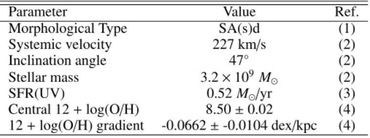
2. Data description

Our target is NGC 7793, a flocculent spiral galaxy (SAd) at a distance ' 3.4 Mpc (Zgirski et al. 2017), located in the Sculp-tor group. Its main properties are summarised in Table 1. NGC 7793 is part of the sample of galaxies studied by the Hubble Space Telescope (HST) Treasury programme LEGUS1_(Calzetti

et al. 2015); the dataset is described in Grasha et al. (2018). Re-cent ALMA data in the CO (J= 2–1) transition provide us with information about the giant molecular cloud (GMC) population at a 0.8500 resolution, and detection limits corresponding to a minimum cloud mass of 104_M

(Grasha et al. 2018). A

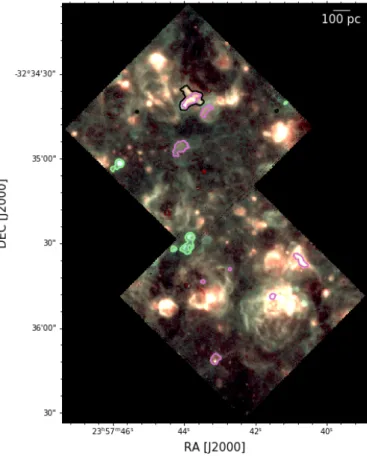
three-colour image from HST and the coverage of the ALMA dataset are shown in Fig. 1.

Within the field of view (FoV) of these two datasets, we have obtained IFU spectroscopy with the MUSE instrument at the ESO Very Large Telescope (VLT) observatory, as part of the Adaptive Optics Science Verification run2. The data were ac-quired in the wide field mode (WFM) configuration with the extended wavelength setting, covering the spatial extent of 1 arcmin2with 0.200sampling and the spectral range 4650 - 9300 Å at 1.25 Å sampling. In the extended wavelength AO mode, the wavelength range ∼ 5760 - 6010 Å is blocked in order to avoid contamination by sodium light from the laser guide system; at our redshift, this rules out several important lines such as the [NII]5755 ‘auroral’ line used for temperature diagnostics. The spectral resolution of the instrument R= λ/∆λ ranges from R = 1770 in the blue end to R= 3590 in the red end of the spectrum. On the final data product, we measure a seeing of 0.7100FWHM (at 4900 Å).

The observation consists of two pointings (centred at R.A. 23:57:42.307, Dec. -32:35:48.150 and R.A. 23:57:43.889, Dec.

1 _{HST GO–13364.}

Table 1. Properties of NGC 7793.

Parameter Value Ref.

Morphological Type SA(s)d (1)

Systemic velocity 227 km/s (2) Inclination angle 47◦ ₍₂₎ Stellar mass 3.2 × 109 _M  (2) SFR(UV) 0.52 M/yr (3) Central 12+ log(O/H) 8.50 ± 0.02 (4)

12+ log(O/H) gradient -0.0662 ± -0.0104 dex/kpc (4)

References. (1) de Vaucouleurs et al. (1991); (2) Carignan & Puche (1990); (3) Calzetti et al. (2015); (4) Pilyugin et al. (2014)

-32:34:49.353, see Fig. 1), each observed during four exposures, for a total of 2100 s on source. In order to take advantage of the seeing enhancement AO performance of MUSE, a Tip Tilt ‘stellar’ like source with brightness in R < 17.5 mag is required within 105" of the MUSE FoV and not closer than 52". The only bright source that could satisfy these technical constraints and allow us to fit the MUSE FoV within the HST–LEGUS coverage and ALMA–LEGUS coverage was the nuclear star cluster in the centre of the galaxy. Four sky frames of 120 s exposure were also acquired in an object-sky-object pattern, located at a distance ∼ 3.8 kpc south-west of the science pointings.

3. Data reduction

3.1. Instrumental signature, flux calibration, and data alignment

The data have been reduced using the MUSE ESO pipeline (Weilbacher et al. 2014, v2.2). We follow the first conventional reduction steps: we combine flat and bias frames into a master frame, we perform wavelength calibration and compute the line spread function (LSF) from the arc-lamps frames. We use a pre-computed geometry table to determine the location of the IFU slices on the FoV and we perform illumination correction com-bining twilight flats. Using the pipeline recipe muse_scibasic, we then combine all this information to remove the instrument signature from science exposures, sky frames and standard star. We perform flux calibration using the standard star and astrom-etry calibration using the astrometric catalogue distributed with the pipeline. We finally run a first time muse_scipost on the object frames to apply these calibrations and remove cosmic ray signatures.

As a last step, we create the astrometry for the final dat-acube. Since we are performing sky subtraction with external software (see Sect. 3.2) operating on datacubes rather than on a ‘pipeline-friendly’, pixeltable level, extra steps need to be taken. We match the absolute astrometry of each pointing to the HST LEGUS observations (Grasha et al. 2018), use the pipeline recipe muse_exp_align to compute the relative shifts of the various exposures and produce a cube having the correct as-trometry using muse_exp_combine. We then take a step back and manually adjust the headers of the non-reduced object pixel tables from muse_scibasic in order to correct for the spatial shift. Finally, we run a second time muse_scipost, using the WCS information from the combined cube to ensure that each of the exposures is added on the right location on the output frame. In this way, once the single science exposures are sky-corrected, the corresponding datacubes can be merged together by a simple exposure time-weighted average.

3.2. Improved sky subtraction

We perform sky subtraction using zap (Soto et al. 2016, v2.0). This software implements a principal component analysis (PCA) on each sky frame, that is it decomposes the image in a set of or-thogonal vectors, each accounting for the largest possible vari-ance in the data. It then applies this vector basis to the science image, finds the corresponding eigenvalues for each individual spectrum and finally uses this to subtract the sky signature from the science frame.

We reduce the four sky exposures with similar steps as for the science frames using the muse_scipost pipeline recipe, and obtain four sky cubes. We then create a skymask, to remove eventual contamination from galactic HII regions and bad pixels. We furthermore adopt two additional precautions when running zap. In the first place, we exclude the bluest end of the spec-trum (4600 - 4812 Å) when computing the eigenvectors on the sky cube, as the LSF varies strongly in this range. The excluded wavelength range was determined by inspecting the behaviour of the first 40 principal vectors; for this portion of the spectrum, we compute sky subtraction using the standard pipeline recipe. Sec-ondly, since the software does not perform accurately in the pres-ence of strong emission lines, we clip the most prominent gas emission lines from the target galaxy (Hα, Hβ, [OIII]4959,5007, [NII]6548, 6584) before computing the eigenvalues of the sky vectors on the data. We then run zap on the four sky frames and apply to each science exposure the correction correspond-ing to the nearest sky frame in time. We carefully inspect the resulting principal vectors and variance ratios, as well as the sub-tracted sky emission to ensure no science is subsub-tracted. Finally, we combine the so obtained eight sky subtracted frames using an exposure time weighted average. By comparing the resulting sky subtracted datacube to the one obtained with the standard MUSE pipeline sky subtraction, we observe that our own sky subtraction significantly improves the quality of the final cubes with residual sky lines strongly reduced.

4. Stellar and gas kinematics 4.1. Stellar continuum modelling

In order to correct for stellar absorption, in particular below the Balmer lines, we perform a fit to the stellar continuum. This also allows us to obtain information on the stellar kinematics (see Sect. 4.3). To achieve a sufficiently high signal to noise in the continuum, we spatially bin the data using the Voronoi tessella-tion method described in Cappellari & Copin (2003). We use the weighted Voronoi tesselation (WVT) adaptation of the algorithm proposed by Diehl & Statler (2006). We create several patterns with a signal-to-noise-ratio (S/N) ∼ 40 - 200 in the continuum region 5020 - 5060 Å and a maximum cell width of 100 pixels. We find that the best compromise between goodness of fit and number of bins is achieved with a S/N = 160 over the continuum region (corresponding to a S/N ∼ 40 in narrow stellar absorption features). We then perform spectral fitting using pPXF (Cappel-lari & Emsellem 2004; Cappel(Cappel-lari 2017).

This software models a galaxy spectrum as Gmod(x)= T(x) ∗ L(cx),

where x= ln λ, T are template spectra and L is the line of sight velocity distribution (LOSVD) of the stars. The underlying as-sumption is that any difference between the galaxy spectrum and the templates is purely due to broadening by the LOSVD. The

Fig. 1. Upper panel: Three-colour image from the HST LEGUS data (R: F814W, G: F555W, B: F336W). The white contours indicate the location of the two MUSE pointings, and the green rectangle shows the coverage of the ALMA CO(2-1) data. Bottom: RGB composite of stellar continuum bands (left panel; R: 6750 - 6810 Å, G: 6520 - 6528 Å, B: 4875 - 4950 Å) and of gas emission lines (right panel; R: Hα, G: [SII]6716,6731, B: [OIII]4959,5007) obtained from the two MUSE tiles.

template resolution is matched to the instrumental one by con- volving the templates with a kernel κ defined by LS Finstrument(x, λ)= LS Ftemplates(x, λ) ∗ κ(x, λ).

The best fitting template is determined by maxmizing a penalised likelihood function, with a penalty function describing the devi-ation of the LOSVD from a pure Gaussian shape. We assume a Gaussian instrumental LSF3 and use the most recent simple stellar populations from Charlot & Bruzual (in preparation). In the range 3540 - 7410 Å, these models are largely based on the MILES stellar library (Sánchez-Blázquez et al. 2006) with FWHM ∼ 2.5 Å spectral resolution (Falcón-Barroso et al. 2011) and are extended using synthetic stellar spectra to cover the spec-tral range from 5.6 Å to 3.6 cm as well as hot stars not avail-able in the MILES library (see Vidal-García et al. 2017; Plat et al. 2019; Werle et al. 2019). These models follow the PAR-SEC stellar evolutionary tracks (Bressan et al. 2012; Chen et al. 2015), which include the evolution of both Wolf Rayet and TP-AGB stars, to describe the evolution of stellar populations of 16 metallicities ranging from Z= 0.0005 to 3.5 Zin the age range

from 1 Myr to 14 Gyr in 220 steps. The advantage of these SSP models over other models based on the MILES library is the in-clusion of stellar populations younger than 60 Myr, which are crucial to study the young star-forming regions in our FoV.

We run pPXF on the Voronoi tessellated datacube, masking all the relevant emission lines in the MUSE range, as well as sky subtraction residuals. However, as the red end of the data is too heavily affected by residual sky emission, we limit our fit to the wavelength range 4600 - 7300 Å. We obtain a best-fit to the continuum in each Voronoi bin; in order to determine the stellar population at a spaxel resolution, we then make the simplifying assumption that the stellar population spectrum does not vary -up to a scale factor - within each bin. We find the best scale factor by computing the median distance between the spectrum in each spaxel and the one in the corresponding Voronoi bin (masking all gas emission lines). We then subtract the contribution from the stars and obtain a datacube consisting exclusively of gas emis-sion (in the following we refer to this data product as a ‘gas cube’). A three-colour composite image obtained from the gas cube is shown in Fig. 1.

4.2. Emission lines fitting

We independently fit gas emission lines, using a single compo-nent Gaussian resulting from a convolution of the instrumental LSF with a Gaussian intrinsic broadening profile. We observe that the reduced χ2 _{goodness-of-fit is uniform over the whole}

FoV (with the exception of the brightest HII regions peaks, where the S/N is exceptionally large), indicating that a single component fit is a valid approximation for both the DIG and HII regions within the data. Analogously to the stellar continuum fit (see Sect. 4.1), we Voronoi tessellate the datacube to increase the S/N of the lines. From the gas cube, we produce linemaps by integrating the flux in the spectral region around each line, and use these to create several Voronoi tessellation patterns that we then apply to the cube. We select a tessellation pattern based on our needs: whenever we are performing an analysis for which a reddening correction is required, we create a pattern correspond-ing to a S/N in Hβ ∼ 20, a threshold determined by requiring a sufficiently small uncertainty in the extinction determined from the Balmer decrement (see Sect. 5); otherwise, we require a S/N ∼ 20 in the weakest line of interest. The selected pattern is ap-plied to the datacube before fitting the emission lines required for the analysis.

3 _{We use the parametrization of the MUSE LSF by Guérou et al.}

(2017): σLS F= 6.266 × 10−8λ2− 9.824 × 10−4λ + 6.286.

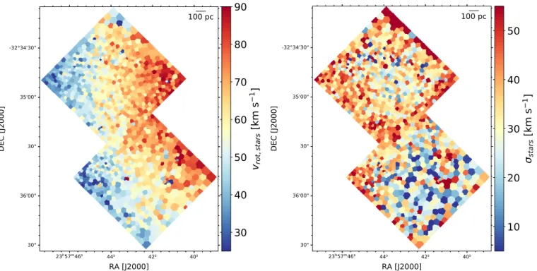
4.3. Velocity and velocity dispersion maps

In Fig. 2 we show the stellar LOSVD parameters v, σ resulting from the fit to the stellar continuum (see Sect. 4.1). Fig. 3 shows the morphology and kinematics of the Hα line, obtained by fit-ting a single Gaussian component to the line (Sect. 4.2). With the assumed instrumental LSF parametrization (see Sect. 4.1), LSF(λHα,obs) ≈ 2.54 Å. Since emission lines have a total

broad-ening

σtot =

q σ2

LS F+ σ2gas,

this sets a lower limit to the gas velocity dispersion we can mea-sure to ∼ 1 Å ≡ 46 km/s. The observed velocity is corrected for an inclination i of 47 degrees and a systemic velocity of 227 km/s (Carignan & Puche 1990) as follows:

vrot = (vobs−vsyst)/sin(i).

The difference in spatial resolution (caused by a different Voronoi tessellation) between stars (Fig. 2) and gas (Fig. 3) is due to the necessity of reaching an optimal S/N on the contin-uum and emission line respectively before fitting.

The velocity fields of stars and gas (left panels of Fig. 2 and 3 respectively) show similar features; we are observing the re-ceding side of the galaxy, and we can see the rotational velocity increase towards the outer part of the disc. The observed velocity range is in agreement with the previous deep Hα observations by Dicaire et al. (2008). The stellar velocity dispersion (right panel of Fig. 2) does not show sharp variations over the whole FoV, but is generally lower in the southern pointing, probably due to the presence of the largest HII region complexes, affecting the stellar light. In the velocity dispersion map of the Hα line we observe instead some regions with a higher σ, clearly standing out against the background, and not coincident with HII regions; we investigate their origin in Sect. 6.2.

5. Reddening estimate

We estimate a reddening map using Pyneb (Luridiana et al. 2015) and the Hα/Hβ ratio, obtained from fitting the gas cube tessel-lated to a S/N ∼ 20 in Hβ. We assume an extinction law k(λ) from Cardelli et al. (1989) and a theoretical Balmer decrement (Hα/Hβ)int = 2.863, corresponding to case B recombination

with Te= 1 × 104K and ne= 1 × 102cm−3(Osterbrock &

Fer-land 2006). It has to be remarked that this assumption describes a foreground screen for the dust, adequate for HII region emis-sion but less accurate in case of spatially extended emisemis-sion, as it can be the case in the DIG. However, we would like to point out that in this work a reddening estimate is used only to correct the [OIII]/Hα line ratio when identifying candidate PNe.

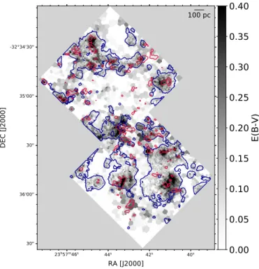
In Fig. 4 we show the resulting extinction map E(B-V), with overlaid GMC contours from the ALMA CO(2-1) data. We can observe that the position of the GMCs is clearly correlated with the higher extinction measured from the Balmer decrement. By comparing this map with the outer boundaries (blue contours) of HII regions (determined in Sect. 6.1), we observe that dense gas clouds with a mass above 104_M

are still coincident (along

the line of sight) with many of the HII regions present in the FoV, suggesting that the dense and ionised gas phases can coexist during the first Myr of evolution. Some regions exhibit a strong extinction but no star formation: these are the locations where the next generation of stars is expected to form.

23h₅₇m₄₆s ₄₄s ₄₂s ₄₀s -32°34'30" 35'00" 30" 36'00" 30"

RA [J2000]

DEC [J2000]

100 pc

30

40

50

60

70

80

v

ro

t,s

ta

rs

[k

m

s

1

]

RA [J2000]

DEC [J2000]

100 pc

10

20

30

40

50

sta

rs

[k

m

s

1

]

Fig. 2. Stellar v and σ parameters of the LOSVD recovered by fitting the stellar continuum with pPXF.

23h₅₇m₄₆s ₄₄s ₄₂s ₄₀s -32°34'30" 35'00" 30" 36'00" 30"

RA [J2000]

DEC [J2000]

100 pc

30

40

50

60

70

80

90

v

ro

t,H

[k

m

s

1

]

RA [J2000]

DEC [J2000]

100 pc

50.0

52.5

55.0

57.5

60.0

62.5

65.0

67.5

70.0

[k

m

s

]

Fig. 3. Velocity and velocity dispersion of the Hα line obtained from a single Gaussian component fit to the line. The instrumental LSF sets a limit for the lowest gas velocity dispersion measurable ∼ 50 km/s.

6. Structure of the ionised gas 6.1. HII regions selection

In the literature a variety of approaches are used to separate HII regions from DIG, relying mainly on the properties of the Hα emission. Widely used are hiiphot, a method proposed by Thilker et al. (2000), based on the gradient of the Hα surface brightness, and the selection criterion proposed by Wang et al. (1998), which defines the boundary between DIG and HII regions according

to the ratio between the local and the mean (at half-light ratio) Hα luminosity. We adopt a slightly different approach, and base our selection on the Hα surface brightness and on characteristic emission line ratios, similarly to what presented by Kreckel et al. (2016). We start by selecting Hα bright regions using the Python package astrodendro4. This tool allows to organise data into a hierarchical tree structure. We input the Hα map obtained by integrating the gas cube in the rest frame wavelength range 6559

23h₅₇m₄₆s ₄₄s 42s 40s -32°34'30" 35'00" 30" 36'00" 30" RA [J2000] DEC [J2000] 100 pc

0.00

0.05

0.10

0.15

0.20

0.25

0.30

0.35

0.40

E(B-V)

Fig. 4. E(B-V) extinction map. Overlaid are the contours of GMCs de-tected with ALMA (red) and of HII regions (blue; this work).

6568 Å. To determine the depth of the tree, we assume a Gaus-sian shape for the diffuse radiation and estimate its median m and standard deviation σ directly on the map via sigma clipping. We compute the dendrogram down to m+10σ (corresponding to a flux of 6.7 × 10−18_{erg s}−1_cm−2_spaxel−1_{) and require a leaf to}

comprise a minimum of 15 pixels, just above the resolution limit. Various limits have been tested for the depth of the dendrogram, in the range (m+ 5σ, m + 20σ); the optimal value has been deter-mined by visual inspection. Our cutoff value corresponds to an emission measure5(EM) of 82 pc cm−6. For reference, Ferguson et al. (1996) used a very similar limiting value of 80 pc cm−6to separate DIG from HII regions in the study of NGC 7793 and NGC 247, whereas Hoopes et al. (1996) used a fainter DIG limit of 50 pc cm−6 _{in the sculptor galaxies NGC 55, NGC 253, and}

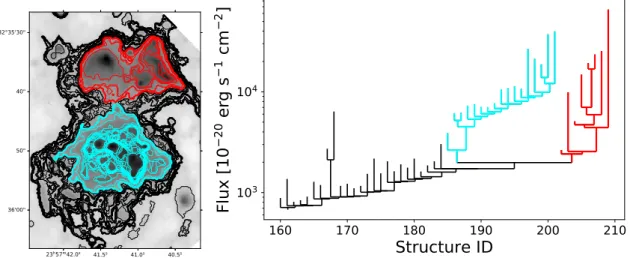
NGC 300. This selection method results in a sample of bright re-gions (leaves) organised into structures (branches), as shown in Fig. 5. In Fig. 6 we show an example region (left panel) and the corresponding dendrogram (right panel). The dendrogram con-sists of a main branch (thick black boundary) and several sub-branches and leaves (thin black lines). The main branch splits in two main sub-branches, highlighted in red and cyan. In the fol-lowing, we refer to the main branches as ‘HII region complexes’, to their upper distinct sub-branches as ’HII regions’ and to leaves as ‘peaks’ inside the HII regions.

Selecting structures based on their brightess, however, does not provide information about the ionisation state of the gas. In order to exclude potential contaminants, we therefore inspect the location of dendrogram structures in the ‘BPT’ line ratio di-agrams [OIII]5007/Hβ vs [NII]6548/Hα and [OIII]5007/Hβ vs [SII]/Hα (Baldwin et al. 1981). This type of diagram was ini-tially devised as a way to separate star forming galaxies from

ob-5 _{The emission measure (EM) is defined as EM := R}L

0 n 2

edl, where ne

is the electron density and L is the total path length of ionised gas. For

a temperature T = 104 _{K, the relation between EM and Hα surface}

brightness is given by: EM [pc cm−6_{]= 4.908 × 10}17_I

Hαerg s−1cm−2

arsec−2_{(Zurita et al. 2000).}

23h₅₇m₄₆s ₄₄s ₄₂s ₄₀s -32°34'30" 35'00" 30" 36'00" 30"

RA [J2000]

DEC [J2000]

100 pc

2.0

2.5

3.0

3.5

4.0

4.5

log

f(

H

)

[1

0

er

g

s

cm

]

Fig. 5. Hα bright regions (white contours) identified with astrodendro overlaid on the Hα linemap. Single regions (leaves) are organised into a hierarchical tree consisting of various branches.

jects primarily excited by other mechanisms (e.g. AGNs), but is also useful to investigate the ionisation state of resolved ISM gas. It is sensitive to parameters such as the hardness of the radiation field, the electron density and the metallicity of the gas (see e.g. Kewley et al. 2006). The resulting diagrams are shown in Fig. 7. Each circle represents detected leaves and branches, whose flux is the total flux of the enclosed spaxels obtained from Gaussian fitting to the line. We would like to point out that also all sub-structures of the tree and not only main branches are included. We compare the position of the regions with models of low metallicity star forming galaxies from Levesque et al. (2010). We adopt the instantaneous burst model grids with an electron density ne= 100 cm−3, in the typical range for HII regions (see

e.g. Osterbrock & Ferland 2006). The models cover the metal-licity range Z = 0.001 − 0.04 and ionisation parameter range q= 1 × 107− 4 × 108cm s−1. We observe that the full range of models, with ages ranging from 0 to 5 Myr, overlaps at least in part with the data, suggesting that an age range is present in the powering sources of the HII regions. We consider as upper limit the 0 Myr grid shown in Fig. 7, which also follows best the dis-tribution of the observed points. We flag structures lying> 0.1 dex above the grid in both BPT diagrams (marked as blue stars in Fig. 7); these regions are analysed in Sect. 6.2. For compari-son, the black dashed line indicates the ‘extreme starburst line’ from Kewley et al. (2001). We observe that our data are better represented by slightly sub-solar metallicity models, and by a ionisation parameter q< 4 × 107cm s−1.

We further inspect two additional line ratios: [OIII]5007/Hα, highlighting high excitation objects, such as planetary nebu-lae (PNe), and [SII]6731/Hα, enhanced in supernova remnants (SNR). From a sample of PNe in local galaxies, Ciardullo et al. (2002) inferred a typical ratio [OIII]5007/Hα > 2, whereas to separate shock-heated SNR nebulae from photoionised gas, the canonical value in the Milky Way and in local group galaxies is

23h₅₇m_42.0s _41.5s 41.0s 40.5s -32°35'30" 40" 50" 36'00"

160

170

180

190

200

210

Structure ID

10

10

Flu

x [

10

20

er

g

s

1

cm

2

Fig. 6. Example of a tree structure constructed with astrodendro on an HII region complex. The left panel shows the structure and the right panel the corresponding tree. Highlighted in cyan and red are the two main distinct branches (‘HII regions’) and their respective sub-structures.

[SII]6731/Hα > 0.4 (see e.g. Blair & Long 1997). Since our tar-get has a lower metallicity, both ratios are suppressed, as we can observe when comparing the Levesque et al. (2010) model grid with the Kewley et al. (2001) extreme starburst line in Fig 7. We therefore inspect all regions featuring a ratio in [OIII]/Hα (PN candidates) and [SII]/Hα (SNR candidates) that is above the 95 percentile of the line ratio observed over the whole FoV. Regions flagged with this method are shown as filled coloured stars in Fig. 7. We observe that almost all of these structures also stand out in the BPT analysis. The spatial location of all the flagged regions is shown in Fig. 8. We investigate their nature further in Sect. 6.2. We note that one of the regions will result to be as-sociated with a WR star and is kept in the HII regions sample. The resulting sample of HII region is shown in Fig. 9 (upper left panel). We also show the total luminosity of the HII-complexes (lower left panel), to offer a comparison with similar studies at larger distances (e.g. Weilbacher et al. 2018).

6.2. Selection of PNe, SNRs and WR star candidates In Sect. 6.1 we have inspected the ionisation state of Hα bright regions and flagged some showing peculiar line ratios. Here we further analyse their nature and build a sample of candidate PNe, SNRs, and WRs.

We have identified regions of high excitation based on their [OIII]5007/Hα ratio. We inspect whether the latter also ex-hibit narrow HeII 4686 line emission, indicating a very strongly ionised medium, in which case we include them in a sample of candidates PNe. We identify two candidates, whose location is shown overlaid on the HeII linemap in Fig. 10. One of the two exhibits a very strong HeII emission as well as a high Hα ve-locity dispersion σ ∼ 85 km/h (see Fig. 11). We would like to point out that since PNe are not resolved at our distance, we do not necessarily expect them to stand out in a velocity dis-persion map. We extract spectra of the candidate using a circu-lar aperture of 0.400, corresponding to the resolution limit (see Fig. A.1): on the extracted spectra we measure an apparent mag-nitude m[OIII]5007 = 25.70 and 23.92 respectively for candidate

PN1 and PN2 in Table 2. Our result does not change if we extract the candidates with astrodendro directly on the [OIII]4959,5007 linemap and with a minimum leaf size corresponding to the res-olution limit.

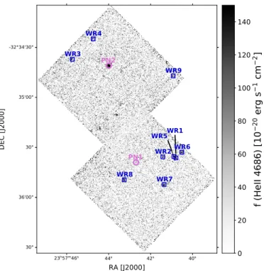
We then inspect regions with a high [SII]6731/Hα ratio to search for SNR candidates. Three of these also show a high Hα velocity dispersion of ∼ 75 − 100 km/s (Fig. 11); we con-firm these as candidate SNR. The position of the candidates is shown in Fig. 11: two of these were previously catalogued by Blair & Long (1997) (with position revised in Pannuti et al. 2001), using Hα and [S II] narrowband filters and the require-ment Hα/[SII] > 0.4. Pannuti et al. (2001) also lists another op-tical candidate in our FoV. Although we do observe a higher line ratio [SII]6731/Hα ∼ 0.24 and an enhanced gas velocity disper-sion at the corresponding location, this region does not make our cut. Also in this case, results do not change if we extract the candidates with astrodendro directly on the [SII]6731 linemap. On the HeII 4686 linemap we also extract WR star can-didates. We run astrodendro with a minimum pixel size of 10 pixels, corresponding to the resolution limit, and down to 40σ above the map background (corresponding to a flux of ∼ 1.0 × 10−18_{erg s}−1_cm−2_{) to extract only the brightest regions.}

We then confirm visually the presence of the characteristic HeII 4686 bump (see spectra in Fig. A.3). This line profile is an indi-cation of stellar winds and clearly distinguishes WR stars from the narrow HeII 4686 emission of PNe. We note that another characteristic feature of WR stars, the CIV 5808 bump, falls inside the AO laser gap for our target. We identify nine WR stars (see Fig. 10), of which seven were never catalogued be-fore. Bibby & Crowther (2010) previously identified three can-didate WR in the MUSE FoV; we confirm two of these (see last two columns of Table 2). We do not observe any HeII emis-sion at the location of the third candidate (ID 20 in Bibby & Crowther 2010). Wofford et al. (2020) select candidate lumi-nous blue variable (LBV) stars combining the LEGUS-HST data with the MUSE dataset presented in this work and independently identify four of the candidates WRs presented here. We see that one of the Hα bright regions flagged in Sect. 6.1 due to its high [OIII]5007/Hα ratio is associated with a WR star.

WR, SNR and PNe candidates are listed in Table 2. Spectra of all the candidates can be found in the Appendix (Fig. A.1, A.2 and A.3). We do not identify the origin of the remaining regions highlighted in Fig. 8, and we label them as ‘regions ionised by other mechanisms’ in the rest of our analysis, as they exhibit features typical of shocked regions.

1.2

1.0

0.8

0.6

0.4

0.2

log

([NII]6584 / H )

1.00

0.75

0.50

0.25

0.00

0.25

0.50

0.75

1.00

log

([

OI

II]

50

07

/

H

)

Z0.004

Z0.008

Z0.02

q1e7

q2e7

q4e7

q8e7

q1e8

q2e8

q4e8

1.25 1.00 0.75 0.50 0.25 0.00

log

([SII]6716,31/ H )

1.0

0.5

0.0

0.5

1.0

log

([

OI

II]

50

07

/

H

)

[OIII]5007/H > 0.5

[SII]6731/H > 0.4

Fig. 7. Location of the Hα bright regions illustrated in Fig 5 on BPT diagnostic diagrams. The coloured grid indicates the models for low metallicity

SF galaxies from Levesque et al. (2010) (0 Myr instantaneous burst with ne= 100 cm−3); the black dashed line shows for reference the extreme

starburst line from Kewley et al. (2001). Circles and stars correspond to regions in Fig. 5; blue stars indicate regions located> 0.1 dex from the

Levesque model grid in both diagrams; filled stars indicate regions with a high ratio of [OIII]5007/Hα (orchid) or [SII]6731/Hα (green).

Fig. 8. Spatial location of the Hα bright regions that show inconsistency with models of star forming galaxies (in black; star symbols in Fig. 7)

or having a ratio [OIII]5007/Hα > 0.5 or [SII]6731/Hα > 0.4 (orchid

and green respectively; filled stars in Fig. 7) overlaid on an RGB image of the gas emission (R: Hα, G: [SII]6716,6731, B: [OIII]4959,5007).

6.3. Testing different ways to select HII regions

As a way of comparison, we perform a different selection pro-cedure to extract HII region boundaries, using the line ratio map Hα/[SII], as in Kreckel et al. (2016). Such analysis is only

possi-Table 2. SNRs, PNe and WRs identified in the MUSE FoV and refer-ence to previous detections. Spectra of all candidates can be found in the Appendix.

Obj. ID Ra (J2000) Dec (J2000) Ref. Ref. ID SNR1 23:57:43.82 -32:35:27.8 1 N7793-S6 SNR2 23:57:45.80 -32:35:01.9 1 N7793-S10 SNR3 23:57:44.00 -32:35:32.1 PN1 23:57:42.71 -32:35:39.2 PN2 23:57:44.01 -32:34:41.2 WR1 23:57:40.81 -32:35:36.5 2 10 (WN2-4b) WR2 23:57:41.43 -32:35:35.9 2 14 (WC4) WR3 23:57:45.74 -32:34:37.4 WR4 23:57:44.75 -32:34:25.1 WR5 23:57:40.90 -32:35:35.6 WR6 23:57:40.53 -32:35:33.1 WR7 23:57:41.37 -32:35:52.5 WR8 23:57:43.27 -32:35:49.6 WR9 23:57:40.94 -32:34:47.3

References. (1) Pannuti et al. (2001); (2) Bibby & Crowther (2010)

ble thanks to the fact that we detect both lines with a sufficiently high S/N across the whole FoV (Hα with S/N > 5 and the com-bined [SII]6716,6731 lines with S/N > 3). This ratio is sensitive to the ionisation state of the gas, due to the slightly lower ioni-sation potential of SII (10.4 eV vs 13.6 eV for HII), and allows us to define better physically motivated HII regions boundaries. Pellegrini et al. (2012) adopts a similar approach, combining Hα emission and the [SII]/[OIII] ratio, to identify HII regions in the LMC and SMC. This approach proves to be effective especially in the case of a density bounded region. We use the same Hα map as in Sect. 6.1 and create a high resolution [SII] map by integrating the gas cube in the rest frame range 6713 6721 and 6728 -6735 Å. We construct a dendrogram on the Hα/[SII] linemap to a depth of 5 σ above the diffuse background mean (corresponding to a line ratio of 2.1) and then follow the same steps described in Sect. 6.1 to obtain a similar HII regions sample. The result-ing regions are shown in Fig. 9 (upper right panel). We see that

23h₅₇m₄₆s ₄₄s ₄₂s ₄₀s -32°34'30" 35'00" 30" 36'00" 30"

RA [J2000]

DEC [J2000]

100 pc

2.0

2.5

3.0

3.5

4.0

log

f(

H

)

[1

0

er

g

s

cm

]

RA [J2000]

DEC [J2000]

100 pc

0.0

0.1

0.2

0.3

0.4

0.5

0.6

log

f(

H

) /

f(

[S

II]

67

16

,3

1)

RA [J2000]

DEC [J2000]

100 pc

0

1

2

3

4

5

6

7

8

L(

H

) [

er

g

s

]

1e38

RA [J2000]

DEC [J2000]

100 pc

0

1

2

3

4

5

6

7

L(

H

) [

er

g

s

]

1e38

Fig. 9. HII regions samples constructed on the Hα map (left) and Hα/[SII] map (right). Top: outermost regions contours (black) overlaid on the linemap; bottom: total luminosity of the regions. One can notice that the Hα/[SII]-selection results in a more conservative sample.

this approach results in a more conservative sample: the bound-aries of the regions are moved to include only gas that exhibits a higher degree of ionisation. This yields, therefore, a larger value for the DIG contribution to the total Hα luminosity within our FoV: we discuss this point in Sect. 8. For the remainder of this work we use the regions selected on the Hα map as a reference.

7. Electron temperature and density

We determine the electron temperature (Te) and density (ne)

of the ionised gas across our FoV with Pyneb (Luridiana et al. 2015). The relation between the ratio of [SIII]6312/9069 and the temperature is shown in Fig. 12 (first two panels); it is apparent that the values of nerelevant to our study (ne<< 1000 cm−3) are

in the regime where every collisional excitation if followed by spontaneous radiative decay and the temperature is independent from the density. For the temperature determination we assume

23h₅₇m₄₆s ₄₄s ₄₂s ₄₀s -32°34'30" 35'00" 30" 36'00" 30" RA [J2000] DEC [J2000] WR1 WR2 WR3 WR4 WR5 WR6 WR7 WR8 WR9 PN1 PN2 0 20 40 60 80 100 120 140

f (

He

II 4

68

6)

[1

0

er

g

s

cm

]

Fig. 10. HeII 4686 linemap obtained by integrating the full cube (gas and stars) in the rest frame wavelength range 4682 - 4691 Å and man-ually subtracting the continuum. The location of identified WR stars is marked in blue; the one of candidate PNe in orchid.

23h₅₇m₄₆s ₄₄s ₄₂s ₄₀s -32°34'30" 35'00" 30" 36'00" 30" RA [J2000] DEC [J2000] PN1 PN2 SNR1 SNR2 SNR3 50.0 52.5 55.0 57.5 60.0 62.5 65.0 67.5 70.0 H

[k

m

s

]

Fig. 11. Velocity dispersion of the Hα line (same as Fig. 3). Overlaid are the HII regions contours (blue; sample selected on the Hα map) and the location of candidate PNe (orchid) and SNR (green).

a fiducial constant density value ne∼ 10 cm−3. We obtain maps

of the two [SIII] lines by integrating respectively the gas cube in the rest frame wavelength range 6310 - 6317 Å and a con-tinuum subtracted cube obtained by extrapolating the best ppxf solution beyond the range of the fit in the wavelength range 9064 - 9077 Å. We tessellate the resulting ratio map to a S/N ∼ 3 in

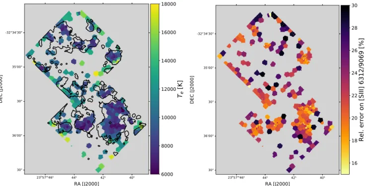
[SIII]6312. We then consider only the Voronoi bins in which the relative error on the [SIII] line ratio is below 30 % (see the right panel of Fig. 13). The main limitation, however, lies in the detec-tion of the weak [SIII]6312 line. Fig. 13 (left panel) shows the re-sulting temperature map. For each Voronoi bin we run pyneb on 1000 Montecarlo realisations of the line ratio, sampling a Gaus-sian distribution with width equal to the 1σ error on the ratio. We estimate an uncertainty on the temperature in each Voronoi bin adopting as upper and lower limit the 14th and 86th percentile of the resulting temperature distribution.

We compare the temperature map to the location of the HII regions and recover a temperature Te = 8714+1319−903 K in HII

re-gions and Te = 12087+1880₋₁₇₁₈ K in the DIG, where we have

in-dicated the median and the first and third quartile of the distri-bution. Hereby we have excluded bins with unrealistically high temperatures Te > 18000 K, all caused by spurious detections

on the edge of the field. This is in line with observations of the Milky Way, where several studies have shown that the tempera-ture of the diffuse gas is ∼ 2000 K higher than in HII regions (see e.g. Haffner et al. 2009; Madsen et al. 2006). In general, we ob-serve a larger spread towards high temperatures in lower surface brightness regions. This seems to indicate a trend of increas-ing temperature with decreasincreas-ing surface brightness, as shown in Fig. 14. However, since we are mainly limited by the ability to detect the weaker [SIII]6312 line, we cannot rule out the exis-tence of a population of lower Hα surface brightness regions at low Te.

We observe two density-sensitive lines in our data, [SII]6731 and [SII]6716. Before computing the line ratio, we bin the faintest line ([SII]6731) to cells with a S/N = 20. The same pattern is then applied to the other [SII] line. The recovered errors on the line ratio are below 7% over all the FoV (right panel of Fig. 15). We compute the density assuming a tempera-ture Te∼ 8000 K, corresponding to the median value observed

across the FoV. The resulting density map is shown in Fig. 15 (left panel). Densities range from 1 to 120 cm−3, with an al-most identical distribution for the DIG and HII regions. More than 50% of bins within both HII regions and DIG remain with undetermined densities because the line ratio is below the sensi-tivity limit of the method. This is illustrated in the bottom panel of Fig. 12, where we show the relation between the line ratio and density as well as the range of observed values in the DIG (in green) and within the boundaries of the HII regions (in purple). The method is unable to recover densities below 1 cm−3

(corre-sponding to a line ratio [SII]6716/6731 ∼ 1.45), and is largely insensitive in the range ne< 30 ([SII]6716/6731 . 1.40). Fig. 16

shows indeed that, within 1σ uncertainty on the line ratio, 81% of the bins are consistent with ne ≤ 1 cm−3, as well as 72% are

consistent with a density of ∼ 30 cm−3_{. This suggests that the}

gas densities within our FoV are largely consistent with densi-ties below ne ≤ 30 cm−3. Subtracting a median DIG spectrum

from HII regions to account for diffuse emission on top of the regions does not impact our results. The inset panel in the upper right corner of Fig. 15 shows a zoom-in into the planetary nebula candidate PN2 (see Table 2). Densities at the location of the neb-ula and in the immediate surroundings are in the range 250-400 cm−3, in agreement with the lower range probed by recent high-resolution studies of planetary nebulae in the Milky Way (see e.g. Walsh et al. 2018; Monreal-Ibero & Walsh 2019).

8. Properties and origin of the DIG

In Sect. 6, we have classified the Hα emitting gas into HII re-gions, bright regions ionised by other mechanisms (e.g by PNe

0

2

4

6

8

log(n

) [cm

]

6000

8000

10000

12000

14000

16000

T

[K

]

6000 8000 10000 12000 14000 16000 18000

T

[K]

0.000

0.025

0.050

0.075

0.100

0.125

0.150

0.175

[S

III]

6

31

2/

90

69

Å

Ne=10 cm-3

observed ratio HII regions

observed ratio DIG

0.0 0.5 1.0 1.5 2.0 2.5 3.0 3.5 4.0

log n

[SII] 6716/6731

observed ratio HII regions observed ratio DIG

1.400 1.425 1.450 1.475 1.500

Fig. 12. Top: Emissivity grid for the [SIII]6312/9069 line ratio, from

pyneb. For densities nebelow the critical value log ne/ 3, the

tempera-ture is almost independent from the density. Centre and bottom: depen-dence of the [SIII]6312/9069 line ratio on the electron temperature and of the [SII]6716/6731 line ratio on the electron density, for a fixed value of the second quantity. Shaded areas indicate the range of observed val-ues for the HII regions (purple) and DIG (green). The coloured area spans the first to third quartile of the distribution; the median is indi-cated as a dotted line. The method is unable to recover densities below

1 cm−3_{(corresponding to a line ratio [SII]6716/6731 . 1.45).}

and SNR) and DIG. Here we investigate the properties of the diffuse gas component.

By inverting our HII regions mask, we find a DIG fraction fDIG ∼ 27% (42 %) for regions selected on the Hα (Hα/[SII])

map. Our two selection methods provide a lower and upper limit to the fDIG. We study the ionised gas in resolved BPT diagrams.

In the [NII]- and [SII]-BPT diagrams in Fig 17, each point corre-sponds to a spatial pixel (spaxel), and is colour-coded according to its belonging to an HII region, a region ionised by a di ffer-ent mechanism (see Sect. 6.2) or the diffuse emitting gas. The

galaxies from Levesque et al. (2010) (see Sect. 6.1) and to fast radiative shock models from Allen et al. (2008). For the latter, we use the models with LMC metallicity (Z ∼ 0.008) and ne = 1,

covering the range b= (0.001 − 100) µG and vshock= 100 - 1000

km/s. Shock-only models are considered for vshock < 200 km/s;

otherwise the full shock+precursor models are used. We observe that: firstly, the DIG exhibits enhanced [SII]/Hα and [NII]/Hα ratios, as observed in the Milky Way and other local galaxies (see e.g. Haffner et al. 2009). Secondly, the bulk of the DIG is either consistent with the models from Levesque et al. (2010) ([NII]-BPT) or just beyond the range spanned by the models, but below the extreme starburst line from Kewley et al. (2001) ([SII]-BPT). Lastly, the fast shock models from Allen et al. (2008) par-tially overlap with the regions featuring strong [OIII]5007/Hα and [SII]6731/Hα line ratios (colour-coded as ‘other ionising source’ in Fig 17) as well as with some of the HII regions spax-els, but show very little overlap with the DIG regions. Using different assumptions for the metallicity and electron density in the shock models does not change this result.

We also investigate the kinematics of the DIG. In Fig. 18 we plot a similar BPT diagram as in Fig. 17, but colour-code all spaxels by their Hα velocity dispersion; the addition of the line of sight velocity dispersion as an ulterior parameter in the BPT diagram has been recently proposed by Oparin & Moiseev (2018). In agreement with their work, we observe a clear trend between velocity dispersion and strength of the radiation field. In general, we observe that spaxels in other ionising sources (marked as stars in Fig. 18) exhibit the highest velocity disper-sions, confirming that they are shock-dominated regions. Spax-els within HII regions have lower velocity dispersion than spax-els located outside. We also observe that spaxspax-els labelled as DIG do overlap with HII region spaxels but have a larger range of velocity dispersion, as confirmed by Fig. 19.

Finally, in Fig. 11, we compare the location of the HII re-gions to the velocity dispersion of Hα, and in Fig 19 we show a histogram of the velocity dispersion measured in HII regions and DIG spaxels. We recover σHα,HII = 52.5+2.1_−1.8 km s−1 and σHα,DIG = 55.6+2.7_−2.3km s−1, where we have indicated the median and the first and third quartile of the distribution. A two-sample Kolmogorov–Smirnov (KS) statistical test recovers a p-value ∼ 0, indicating that the two distributions differ. The tail of larger velocity dispersion in the DIG, which is not seen in HII regions, might be an indication of a higher turbulent motion in the ISM, and hinting to the fact that shocks and mechanisms other than photoionisation could still play a non-negligible role in the ion-isation of the DIG. Alternatively, this could be due to a line of sight effect: DIG spaxels might have contributions from gas dis-tributed along the line of sight, originating from regions with a physical separation up to a kpc, whereas HII regions spaxels are dominated by flux originating from a physically narrow region. 9. Conclusions

We have presented recent MUSE AO observations of the nearby galaxy NGC 7793. We produced maps of nebular extinction, electron density and temperature, as well as stellar and gas kine-matics. We analysed the state of the ionised gas and identified its various components: we constructed a sample of HII regions by applying a surface brightness cut in Hα or in the line ratio Hα/[SII], and excluded contaminants by placing the resulting re-gions in BPT diagrams and inspecting their ratio of [OIII]5007 and [SII]6731 with respect to Hα. Using these two line ratios, we also identified two candidates PNe and three SNRs (two of

23h₅₇m₄₆s ₄₄s ₄₂s ₄₀s -32°34'30" 35'00" 30" 36'00" 30" RA [J2000] DEC [J2000] 6000 8000 10000 12000 14000 16000 18000

T

[K

]

Rel. error on [SIII] 6312/9069 [%]

Fig. 13. Left: electron temperature computed with pyneb, for an assumed density ne= 10 cm−3. HII region contours are overlaid in black. Right:

relative error on the [SIII]6312/9069 line ratio. Grey-shaded areas indicate bins where either the [SIII]6312 line was not detected, or the error on

the [SIII] line ratio is> 30%.

3.5

4.0

4.5

5.0

5.5

6.0

6.5

log SB(H ) [10

20

_{erg s}

1

_cm

2

_arcsec

2

_]

6000

8000

10000

12000

14000

16000

18000

20000

22000

T

e

[K

]

HII regions

DIG

other ionizing source

Fig. 14. Electron temperature as function of Hα surface brightness for each Voronoi bin in Fig. 13. Points are labelled according to whether the corresponding Voronoi bin is part of an HII region (purple circles), the DIG (green diamonds) or of a region ionised by another source (grey

stars). Bins with a relative error on the [SIII] line ratio> 30% have been

excluded, as wells as bins with Te> 18000 (spurious detections on the

edge of the FoV).

which previously catalogued as candidates); all SNRs and one of the PNe also exhibit a large Hα velocity dispersion. Finally, we produced a HeII 4686 linemap and identified nine WR stars candidates, seven of which were never catalogued before.

We then investigated the properties and origin of the DIG. Our main findings are as follows: firstly, depending on the sur-face brightness cut applied in the selection of the HII regions, we obtain a DIG fraction fDIG ∼ 27% (Hα) or 42% (Hα/[SII]).

The diffuse gas exhibits enhanced [SII]/Hα and [NII]/Hα ra-tios, indicating its lower ionisation state, as broadly observed

in nearby galaxies. Secondly, pyneb reveals that the line ratio [SII]6716/6731 in the majority of our FoV is consistent within 1σ with electron densities below 30 cm−3, with an almost iden-tical distribution for the DIG and HII regions. The electron tem-perature of the DIG is ∼ 3000 K higher than in HII regions, in agreement with DIG studies in the Milky Way. We moreover observe an apparent inverse dependence of the electron tempera-ture on the Hα surface brightness, consistent with what observed in the Milky Way, where the temperature of the DIG increases for decreasing emission measure (Haffner et al. 2009). However, due to the sensitivity limit in the weak [SIII]6312 line, we can-not rule out the existence of a population of lower Hα surface brightness regions at low Te. Thirdly, by comparing the DIG

emission with models for low metallicity star forming galaxies from Levesque et al. (2010), we observe that the bulk of the DIG emission is consistent with being photoionised or just above the range spanned by the models. We also assess that the fast ra-diative shock models from Allen et al. (2008) show little to no overlap with the DIG spaxels. Finally, we add as third variable in our BPT diagram the line of sight velocity dispersion of the Hα line, as recently proposed by Oparin & Moiseev (2018), and observe a clear trend between the velocity dispersion and the strength of the radiation field. In particular, we find enhanced gas velocity dispersions in the DIG with respect to HII regions, indicating that effects others than photoionisation might play a non-negligible role.

In Paper II, we will combine these results on the ionised gas with the stellar population studied within the HST–LEGUS pro-gramme and the dense gas properties provided by the ALMA-LEGUS data. We will further investigate how the physical prop-erties of HII regions (luminosity, geometry, density or ionisation boundness) relate to the ages and masses of the hosted stellar clusters and the number of massive stars and WR candidates. We will also provide a quantitative estimate of which fraction of the DIG luminosity could be accounted for by ionising radiation escaping HII regions.

23h57m46s ₄₄s ₄₂s ₄₀s -32°34'30" 35'00" 30" 36'00" 30" RA [J2000] DEC [J2000] 10 20 30 40 50

n

[c

m

]

Rel. error on [SII] 6716/6731 [%]

Fig. 15. Left: electron density computed with pyneb, for an assumed temperature Te∼ 8000 K. HII region contours are overlaid in black.

Grey-shaded areas indicate bins where the observed line ratio is below the sensitivity limit of the method (see bottom panel of Fig. 12). The upper right

panel shows a zoom-in into the planetary nebula candidate PN2 (red cross; see Table 2). Right: relative error on the [SII]6716/6731 line ratio. The

recovered values are below 7% over all the FoV.

0.0

0.5

1.0

1.5

2.0

2.5

3.0

/

err

0

200

400

600

800

1000

1200

N bins

/

/

Fig. 16. Absolute distance of the observed [SII] ratio from a value of

1.45 (∆1.45, blue histogram), corresponding to the low density limit ne=

1 cm−3_{, and from a value of 1.40 (∆}

1.40, orange line), corresponding to

a density ne∼ 30 cm−3, expressed in terms of the error on the line ratio

σerr.

Acknowledgements. The authors thank the Anonymous Referee for the helpful comments and constructive remarks on this manuscript. This work is based on observations collected at the European Southern Observatory under ESO pro-gramme 60.A-9188(A). A.A. acknowledges the support of the Swedish Research Council, Vetenskapsrådet, and the Swedish National Space Agency (SNSA). GB acknowledges financial support from DGAPA-UNAM through PAPIIT project IG100319. MF acknowledges support by the Science and Technology Facili-ties Council [grant number ST/P000541/1]. This project has received funding from the European Research Council (ERC) under the European Union’s Hori-zon 2020 research and innovation programme (grant agreement No 757535). AW acknowledges financial support from DGAPA-UNAM through PAPIIT project IA105018. This research made use of Astropy6, a community-developed core Python package for Astronomy (Astropy Collaboration et al. 2013, 2018). PyRAF is a product of the Space Telescope Science Institute, which is operated by AURA for NASA.

6 _{http://www.astropy.org}

References

Allen, M. G., Groves, B. A., Dopita, M. A., Sutherland, R. S., & Kewley, L. J. 2008, ApJS, 178, 20

Astropy Collaboration, Price-Whelan, A. M., Sip˝ocz, B. M., et al. 2018, AJ, 156, 123

Astropy Collaboration, Robitaille, T. P., Tollerud, E. J., et al. 2013, A&A, 558, A33

Bacon, R., Accardo, M., Adjali, L., et al. 2010, in Society of Photo-Optical In-strumentation Engineers (SPIE) Conference Series, Vol. 7735, Proc. SPIE, 773508

Baldwin, J. A., Phillips, M. M., & Terlevich, R. 1981, PASP, 93, 5 Bibby, J. L. & Crowther, P. A. 2010, MNRAS, 405, 2737 Blair, W. P. & Long, K. S. 1997, ApJS, 108, 261

Bressan, A., Marigo, P., Girardi, L., et al. 2012, MNRAS, 427, 127 Calzetti, D., Lee, J. C., Sabbi, E., et al. 2015, AJ, 149, 51 Cappellari, M. 2017, MNRAS, 466, 798

Cappellari, M. & Copin, Y. 2003, MNRAS, 342, 345 Cappellari, M. & Emsellem, E. 2004, PASP, 116, 138

Cardelli, J. A., Clayton, G. C., & Mathis, J. S. 1989, ApJ, 345, 245 Carignan, C. & Puche, D. 1990, AJ, 100, 394

Chen, H.-L., Woods, T. E., Yungelson, L. R., Gilfanov, M., & Han, Z. 2015, MNRAS, 453, 3024

Ciardullo, R., Feldmeier, J. J., Jacoby, G. H., et al. 2002, ApJ, 577, 31 Cole, S., Lacey, C. G., Baugh, C. M., & Frenk, C. S. 2000, Monthly Notices of

the Royal Astronomical Society, 319, 168 Collins, J. A. & Rand, R. J. 2001, ApJ, 551, 57

de Vaucouleurs, G., de Vaucouleurs, A., Corwin, Herold G., J., et al. 1991, Third Reference Catalogue of Bright Galaxies

den Brok, M., Carollo, C. M., Erroz-Ferrer, S., et al. 2019, arXiv e-prints, arXiv:1911.06070

Dicaire, I., Carignan, C., Amram, P., et al. 2008, AJ, 135, 2038 Diehl, S. & Statler, T. S. 2006, MNRAS, 368, 497

Drissen, L., Martin, T., Rousseau-Nepton, L., et al. 2019, MNRAS, 485, 3930 Erroz-Ferrer, S., Carollo, C. M., den Brok, M., et al. 2019, MNRAS, 484, 5009 Falcón-Barroso, J., Sánchez-Blázquez, P., Vazdekis, A., et al. 2011, A&A, 532,

A95

Ferguson, A. M. N., Wyse, R. F. G., Gallagher, J. S., I., & Hunter, D. A. 1996, AJ, 111, 2265

Grasha, K., Calzetti, D., Bittle, L., et al. 2018, MNRAS, 2082 Guérou, A., Krajnovi´c, D., Epinat, B., et al. 2017, A&A, 608, A5

Haffner, L. M., Dettmar, R. J., Beckman, J. E., et al. 2009, Reviews of Modern Physics, 81, 969

Hoopes, C. G. & Walterbos, R. A. M. 2000, ApJ, 541, 597 Hoopes, C. G. & Walterbos, R. A. M. 2003, ApJ, 586, 902

Kewley, L. J., Dopita, M. A., Sutherland, R. S., Heisler, C. A., & Trevena, J. 2001, ApJ, 556, 121

Kewley, L. J., Groves, B., Kauffmann, G., & Heckman, T. 2006, MNRAS, 372, 961

Kreckel, K., Blanc, G. A., Schinnerer, E., et al. 2016, ApJ, 827, 103 Levesque, E. M., Kewley, L. J., & Larson, K. L. 2010, AJ, 139, 712 Luridiana, V., Morisset, C., & Shaw, R. A. 2015, A&A, 573, A42 Madsen, G. J., Reynolds, R. J., & Haffner, L. M. 2006, ApJ, 652, 401 Mathis, J. S. 2000, ApJ, 544, 347

Monreal-Ibero, A. & Walsh, J. R. 2019, arXiv e-prints, arXiv:1912.02847 Oey, M. S., Meurer, G. R., Yelda, S., et al. 2007, ApJ, 661, 801 Oparin, D. V. & Moiseev, A. V. 2018, Astrophysical Bulletin, 73, 298 Osterbrock, D. E. & Ferland, G. J. 2006, Astrophysics of gaseous nebulae and

active galactic nuclei

Pannuti, T., Filipovi´c, M. D., Duric, N., Pietsch, W., & Read, A. 2001, in Ameri-can Institute of Physics Conference Series, Vol. 565, Young Supernova Rem-nants, ed. S. S. Holt & U. Hwang, 445–448

Pellegrini, E. W., Oey, M. S., Winkler, P. F., et al. 2012, ApJ, 755, 40 Pilyugin, L. S., Grebel, E. K., & Kniazev, A. Y. 2014, AJ, 147, 131 Plat, A., Charlot, S., Bruzual, G., et al. 2019, MNRAS, 2242 Rand, R. J. 1998, ApJ, 501, 137

Reynolds, R. J., Haffner, L. M., & Tufte, S. L. 1999, ApJ, 525, L21

Rousseau-Nepton, L., Martin, R. P., Robert, C., et al. 2019, arXiv e-prints, arXiv:1908.09017

Sánchez-Blázquez, P., Peletier, R. F., Jiménez-Vicente, J., et al. 2006, MNRAS, 371, 703

Soto, K. T., Lilly, S. J., Bacon, R., Richard, J., & Conseil, S. 2016, MNRAS, 458, 3210

Thilker, D. A., Braun, R., & Walterbos, R. A. M. 2000, AJ, 120, 3070 Thilker, D. A., Walterbos, R. A. M., Braun, R., & Hoopes, C. G. 2002, AJ, 124,

3118

Vandenbroucke, B., Wood, K., Girichidis, P., Hill, A. S., & Peters, T. 2018, MN-RAS, 476, 4032

Vidal-García, A., Charlot, S., Bruzual, G., & Hubeny, I. 2017, MNRAS, 470, 3532

Walsh, J. R., Monreal-Ibero, A., Barlow, M. J., et al. 2018, A&A, 620, A169 Wang, J., Heckman, T. M., & Lehnert, M. D. 1998, ApJ, 509, 93

Weilbacher, P. M., Monreal-Ibero, A., Verhamme, A., et al. 2018, A&A, 611, A95

Weilbacher, P. M., Streicher, O., Urrutia, T., et al. 2014, in Astronomical Soci-ety of the Pacific Conference Series, Vol. 485, Astronomical Data Analysis Software and Systems XXIII, ed. N. Manset & P. Forshay, 451

Werle, A., Cid Fernandes, R., Vale Asari, N., et al. 2019, MNRAS, 483, 2382 Wofford, A., Ramírez, V., Lee, J. C., et al. 2020, MNRAS[arXiv:2001.10113] Wood, K. & Mathis, J. S. 2004, MNRAS, 353, 1126

Zgirski, B., Gieren, W., Pietrzy´nski, G., et al. 2017, ApJ, 847, 88 Zhang, K., Yan, R., Bundy, K., et al. 2017, MNRAS, 466, 3217 Zurita, A., Beckman, J. E., Rozas, M., & Ryder, S. 2002, A&A, 386, 801 Zurita, A., Rozas, M., & Beckman, J. E. 2000, A&A, 363, 9

Fig. 17. [NII]- and [SII]-BPT diagrams with each spaxel colour-coded based on its spatial location: inside an HII region (purple circles), a region ionised by another source (grey stars) or in the DIG (green diamonds). Observations are compared with fast radiative shock models from Allen

et al. (2008) (shock only models for vshock< 200 in red; shock+precursor models for vshock> 200 in dark blue) and models of star forming galaxies

Fig. 18. As in Fig. 17, each point represents a spaxel; here the points are colour-coded by their Hα velocity dispersion, whereas their shape varies depending on their location within HII regions (circles), DIG (diamonds) or strongly ionised regions (stars). The observed points are compared to

fast radiative shock models from Allen et al. (2008) (shock only models for vshock< 200 in magenta; shock+precursor models for vshock > 200 in

light green), models of star forming galaxies from Levesque et al. (2010) (solid black) and the extreme starburst line from Kewley et al. (2001) (dashed black).

45

50

55

60

65

70

75

H

[km/s]

0.00

0.02

0.04

0.06

0.08

0.10

0.12

0.14

N

HII regions

DIG

Fig. 19. Normalized distribution of the measured Hα velocity disper-sion for spaxels located in HII regions (purple) and in the DIG (green). The coloured area spans the first to third quartile of the distribution; the median is indicated as a dashed line.