Development of laboratory class experiment to characterize magneto-rheological fluid

(1)

Development of Laboratory Class Experiment to

Characterize Magneto-Rheological Fluid

By

Stephen D. Ray

SUBMITTED TO THE DEPARTMENT OF MECHNICAL ENGINEERING IN PARTIAL FULFILLMENT OF THE REQUIRMENTS FOR THE DEGREE OF

BACHELOR OF SCIENCE IN MECHANICAL ENGINEERING AT THE

MASSACHUSETTS INSTITUTE OF TECHNOLOGY June 2008

,K§ZLn

Signature of Author: - ,

Department ofMechanical Engineering

03/21/08 Certified by: Professor of Douglas P. Hart Mechanical Engineering Thesis Supervisor Accepted by:' ohn H. Lienhard V echanical Engineering Chairman, Undergraduate Thesis Committee

MASSACHWSETTS INST E OF TECHNOLOGY

AUG 1

4 2008

LIBRARIES

(2)

ARCHMtLt-Development of Laboratory Class Experiment to Characterize Magneto-Rheological Fluid

By

Stephen D. Ray

Submitted to the Department of Mechanical Engineering on April 2, 2008 in partial fulfillment of the requirements for the Degree of Bachelor of Science in

Mechanical Engineering

ABSTRACT

An experimental apparatus has been developed that characterizes magneto-rheological (MR) fluid for an MIT Mechanical Engineering laboratory class by charting the fluid's yield stress versus magnetic field strength. The apparatus consists of a cantilevered beam

that is damped using MR fluid, through which a magnetic field is varied. Unique functional requirements for a class experiment as well as experimental design rationale are also discussed.

Lord's MRF-336AG MR fluid is characterized at low magnetic field strengths and compared to the company provided data. Experimental data suggest the magnetic field strength affects the fluid yield stress more greatly than the company data, though both data show similar general trends. This discrepancy likely comes from approximations for damper velocity made in the analysis. Both a Bingham plastic and Newtonian model are used to describe the fluid and based on the similarity of the results from both models at

low field strengths, it is concluded that MR fluid can be modeled as a Newtonian fluid for field strengths between 0 and 4 kAmp/m.

Thesis Supervisor: Douglas P. Hart

(3)

1. Purpose

The stated purpose of the 2.672 Project Laboratory class is "to provide experience in formulating, solving, and presenting solutions to engineering problems." To

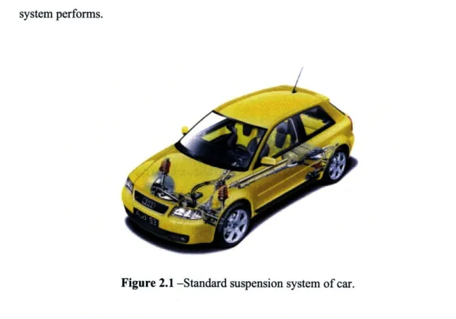
accomplish the this purpose, students analyze a real-world problem and test their analysis using an experiment in the lab. A new experiment has been proposed to model a variable shock system for a car using a small-scale suspension system. A variable shock system is similar to a standard suspension system, like the one shown in Figure 2.1, in that it damps small perturbations incurred by the car tires. However, a variable shock system allows for a "stiffening" of the shocks, which provides more precise control of how the entire system performs.

/

Figure 2.1 -Standard suspension system of car.

Magneto-rheological (MR) fluid will be used to provide the variable damping. My thesis develops an experiment that allows students to characterize the MR fluid that will be used

(6)

for the small-scale suspension system. Given the nature of this thesis that not only characterizes MR fluid, but also designs and builds the apparatus to do so, this report focuses first on the experiment to characterize MR fluid and then on design of the experiment.

2. Introduction

MR fluid technology was first patented by Jacob Rabinow during the middle of the twentieth century, however in its infancy, it was considered more of a laboratory oddity than a technology with practical use. Towards the end of the twentieth century, though, advances in complimentary technology allowed researchers to more seriously consider the commercial viability of MR fluid technology. Since then, MR fluids have been used in a wide variety of applications, such as in prosthetics, seismic protection devices, aerobic machines, precision finished lenses, and in advanced controls, including variable shock systems.

MR fluids are suspensions of micron-sized magnetic particles in a low volatility carrier fluid, typically some kind of hydrocarbon, and undergo changes in their

rheological behavior in the presence of a magnetic field. In this experiment, Lord's MRF-336AG is characterized using a vibrating beam damped by the fluid, which is exposed to a ceramic bar magnetic, whose strength is measured using a gaussmeter. The system's response to vibration is measured by an inductive position transducer. Because MR fluid is often modeled as a Bingham Plastic, the field-dependent yield stress provides the desired variability for a shock system. Thus, to characterize the fluid, the fluid's yield stress as a function of magnetic field intensity is determined.

(7)

3. Theory

3.1 Magneto Rheological (MR) Fluid

With no magnetic field present, MR fluids are modeled reasonably well as Newtonian Fluids. Recall that for Newtonian Fluids, shear stress, 7 , is a function of viscosity, y , and the velocity gradient perpendicular to the direction of shear, or shear rate, y.

= -uy (1)

By definition, the viscosity of a Newtonian Fluid depends only on pressure and temperature, which is approximately true for MR fluids when no magnetic field is present.

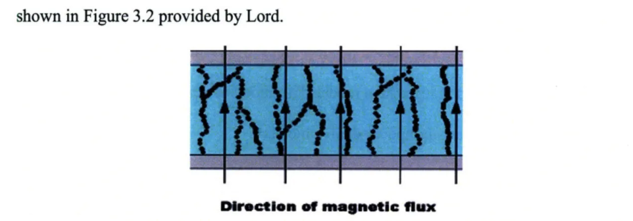
In the presence of a magnetic field, the magnetic particles in MR fluids align, as shown in Figure 3.2 provided by Lord.

I I I I I

Dkrectlem et magnetic flux

Figure 3.1 - Aligning of magnetic particles in MR fluid in presence of magnetic field.

What results is commonly modeled as a Bingham plastic for most engineering purposes. As such, for stresses greater than the yield stress, the shear stress, -r , is a function of the

(8)

shear rate, y, the no-field viscosity, p., and the field-dependent yield stress ,Y (H), where H is the strength of the magnetic field.

r = r,(H) + for r > ,r (H) (2)

For stresses less than the yield stress, the fluid is semi-solid and behaves viscoelastically. Thus, the shear stress is a function of the shear strain y and the complex material modulus G

S-= Gy for r < r, (3)

3.2 System Modeling

3.2.1 System Model

In order to usefully model variable shocks with a small-scale suspension system, one needs to know how the damping fluid in the small-scale damper, MR fluid, varies. The property of interest is the field-dependent yield stress, which is expected to vary with the magnetic field strength. The field-dependent yield stress will be measured using a lumped parameter second order system model. This model is derived from the equation

of motion for a spring-mass-dashpot system, which is

Mx +Cx+Kx=F, (4)

where x is the position of the point mass M at the end of the beam, C is the damping constant, K is the spring constant, and F is the applied force. This model is only valid for a point mass system in which the mass displacement is measured where the force is applied. Due to the complication of a beam with distributed mass, attached plunger for a position transducer, and weight of the damper, this ideal lumped parameter model will be

(9)

adjusted for our use. The following system modeling is heavily taken from ElectroMechanical Experiment Background by Ian Hunter and Barbara Hughey.

3.2.2 Length Factor

To account for the distributed mass, we will assume a linear system and thus can sum the effects of each differential mass element to find the entire system response. To do this, we must know the displacement of each mass element and how it relates to the displacement at the free-end of the beam. The equation below describes the desired displacement, which is that of a cantilevered beam with a load applied at the free end,

x

z

=

z

2

(3L

-

z),

(5)

6E1

Where xz is the beam deflection a distance z from the clamped end, F is the force applied

at the free end, E is the beam modulus of elasticity, I is the beam moment of inertia, and L is the length of the beam. Solving for the free-end displacement, which is the point where z=L, yields

FL3

xL =

FL

₍₆₎

3EI

These two equations, (5) and (6), can be combined to give a lengthfactor lengthfactor = - (3L - z)(7)

XL 2L₃

which provides a way to relate the displacement of an elemental mass element to the free-end deflection.

(10)

3.2.3 System Parameters

Two transfer functions are commonly used to describe a second-order system. The first will be defined using engineering parameters K, M, and C, as mentioned before. They are combined to yield

lengthfactor (8)

n(s) = Ms2 + Cs + K'

where Y(s) is the beam displacement at the position transducer, F(s) is the force applied at the free-end of the beam, and the lengthfactor, as defined in Eq. (7), accounts for the position transducer's not being at the free-end of the beam.

The other transfer function we will use is comprised of what we will call "physics parameters" and is shown here

(9) Gain 0 n 2

Hphs(S)= +2c S + o 2'

where o_n represents the natural frequency, 5 represents the damping ratio, a

the static gain of the system. Combining the two transfer functions yields lengthfactor lengthfactor Gain o 2 M Ms2 + C_S+ K _s2 + 2cOs + o 2 _{2 +} _C + M M md Gain is (10)

By inspection of Eq. (10), it can be found that

2 K " M' 2 _lengthfactor Gain" w M C 2(, n =•-M (11)

Rearranging these equations, we can solve for the physics parameters in terms of the engineering parameters,

(11)

Gain = lengthfactor (12)

K C

Further rearrangement yields the engineering parameters in terms of the physics parameters, K- lengthfactor Gain lengthfactor M2 , (13) Gain.* ,2 C 2. lengthfactor Gain - o,

3.2.4 Experimentally Determining Damping Constant, C

A second-order system is considered underdamped when the damping ratio, ý, is

< 1, which will be the case for the majority of this experiment. Using Eq. (4) with F set to

zero, thus the system is freely vibrating, it can be found that the position, x, of the free end of the beam for an underdamped system is

x = A * e-f "t sin(wodt + #), (14)

where A is a coefficient of fit, od is the damped natural frequency, and 0 is the offset

phase angle. The damped natural frequency is written in terms of C and co, as follows

od = 2.O--. (15)

Inserting Eq. (15) into Eq. (14) yields

(12)

which will be fit to the system response to measure both ý and w,. Once these parameters have been found, they can easily be inserted into Eq. (13) to yield C.

3.3 Fluid Characterization

3.3.1 Newtonian Couette Flow

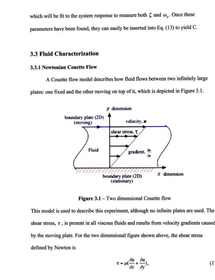
A Couette flow model describes how fluid flows between two infinitely large

plates: one fixed and the other moving on top of it, which is depicted in Figure 3.1.

y dimension boundary plate (2D) (moving) Fluid velocity, R shear stress, T gradient,

-boundary plate (2D) x dimension (stationary)

Figure 3.1 - Two dimensional Couette flow

This model is used to describe this experiment, although no infinite plates are used. The shear stress, r , is present in all viscous fluids and results from velocity gradients caused

by the moving plate. For the two dimensional figure shown above, the shear stress

defined by Newton is

du du

S (-- + -), (17)

(13)

where i is the dynamic fluid viscosity and u(y) is the fluid velocity in the gap. Given our experimental setup, there is no motion in the y-direction, so -=0, thus Eq. (17) becomes

du u(y) (18)

dx

6

where 6 is the gap between the two plates. For a plate of length I and width w, the total shear force, FPN, exerted on the plate by the Newtonian fluid is thus

FpN, = -y( * lw. (19)

Furthermore, by definition of a damping constant,

FpN - C,P, Xpi, (20)

where xp is the plate velocity. With a no-slip boundary condition, the fluid velocity at the plate, u(6), must equal xp, thus Eq (19) becomes

FpN - P * lw. (21)

Equating Eqs. (20) and (21), the damping constant for the plate is found to be

p

- lw

C,1 = (22)

Because the plate is located at the free end of the beam, 20K

C, = C , (23)

(On

where C is the system damping constant defined in Eq. (4). All parameters on the right side of the equation will be experimentally measured, thus giving us an experimentally determined damping constant for a Newtonian Fluid. Once C is obtained from the experiment, M can be found by rearranging Eq. (23) to yield

(14)

C.6

6=

(24)

lw

3.3.2 Impulse Diffusion Time

If the excitation force of the beam is applied as an impulse, it takes some finite

time to propagate through the fluid. By applying momentum conservation and continuity to a flat plate covered with a fluid, Kundu derives the following relationship for the thickness of the diffusive layer at which the fluid velocity falls within 5% of the plate

velocity u

6df,

4-~

- i

.

(25)

In this relationship, tdi is the time it takes for the diffusive effects to propagate a distance 6di, while v is the kinematic viscosity. Given a fixed gap size 6, the time for 95% of the diffusive effects to propagate throughout 6 is thus

(6/4)2

tdif = (26)

V

3.3.3 Experimentally Determining Yield Stress

Substituting the shear stress for a Bingham plastic, Eq. (2), into Eq. (19) in place of the Newtonian definition of shear stress yields the shear force exerted on the plate by a Bingham plastic, FPB,

Fp = -[, (H) +

P

y)]. lw.

(27)

Equating Eq. (27) to the definition of the damping constant, Eq. (20), and solving for

rz(H) yields,

C__6 C-6

T,(H)=(' 6 - y=( - y. (28)

(15)

The no-field viscosity, N, is determined using the Newtonian approach mentioned in

3.3.1, as MR fluids are modeled as Newtonian in the absence of a magnetic field. The

shear rate, y, which has already been mentioned, is defined as

du x_d

S- = - ₍₂₉₎

dy 6

Where xd is the velocity of the damper. Thus, substituting Eq. (29) into Eq. (28),

(H) =C"6 -N)'-Xd (30)

1w 6

Because the damper velocity is not constant, the initial velocity is chosen as a representative value. The initial damper velocity is found by differentiating Eq. (16), which yields

Xd = Aocos(Cw, On-V " t') n 1-t 2 = Ao ' C -• 2 _, ₍₃₁₎

where Ao is the initial peak displacement. Combining Eqs. (31) and (30) gives zry(H) in

terms of all experimentally determined parameters

C-6 A#-o)" "3

S(H) ( -)- A= / (32)

(16)

4. Experimental Setup

4.1 Apparatus

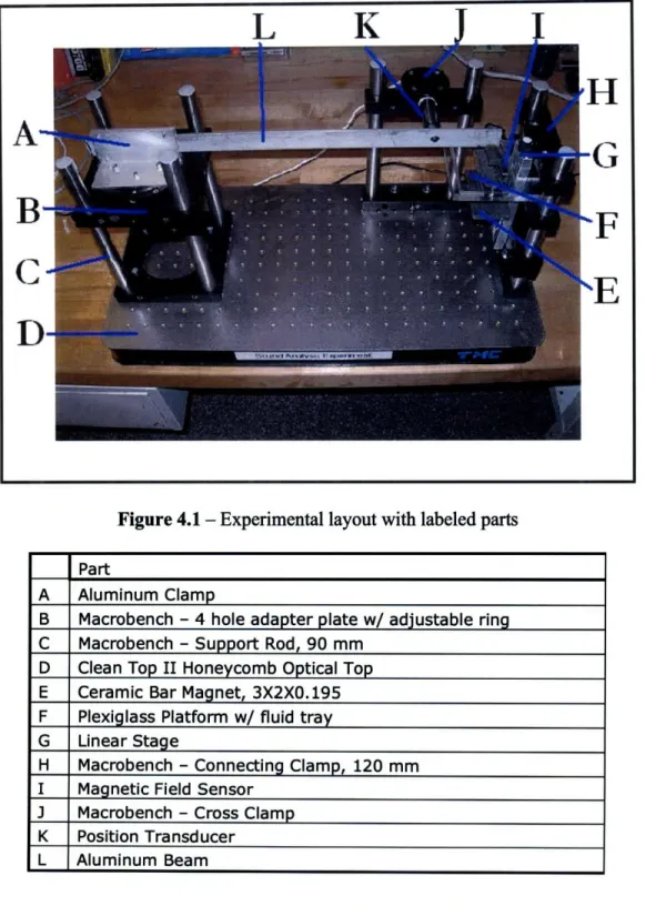
Figure 4.1 shows the overall layout of the experiment and labels key components.

Figure 4.1 - Experimental layout with labeled parts

Part

A Aluminum Clamp

B Macrobench - 4 hole adapter plate w/ adjustable ring

C Macrobench - Support Rod, 90 mm

D Clean Top II Honeycomb Optical Top

E Ceramic Bar Magnet, 3X2X0.195 F Plexiglass Platform w/ fluid tray

G Linear Stage

H Macrobench - Connecting Clamp, 120 mm

I Magnetic Field Sensor

3 Macrobench - Cross Clamp K Position Transducer L Aluminum Beam

LK

II

H

MG

F

"E

A-

B-

(17)

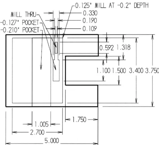
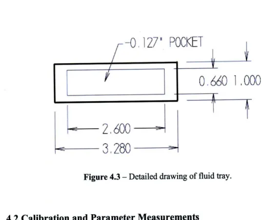
C-Both the plexiglass platform and fluid tray were designed and manufactured at MIT. See Figures 4.2 and 4.3 below for detailed part drawings of the platform and tray

respectively.

MILL T•R-U

-0,127'

POCKET

-0.210'

POCKET--T~1 .'UUb

o-c=

2,700

=

5.000 _:

0,125'

MILL AT -0.2'

DEPTH

0 .330

0.190

0. 109 I .I. S I T'I

0,592 1,318

I -"1- d T

:TL

S1

750 -1j0'

1,1001 .500

Figure 4.2 - Part drawing of the fluid platform, made from 0.465" stock plexiglass.

I;

3,400

3.750

I

t

I

x '

_ r ,,--4 I -,,I I I---,'---- --I 1 I_

I

g

(18)

-0, 127'

2,600

>

3,280

POCKET

0660 1 ,000

...

Figure 4.3 - Detailed drawing of fluid tray.

4.2 Calibration and Parameter Measurements

4.2.1 Calibration of Position Transducer

Using a pair of calipers, the distance from the beam to a fixed location was measured while corresponding voltages were recorded. See Figure 4.4 below for the

calibration setup.

Figure 4.4 - Transducer calibration setup.

(19)

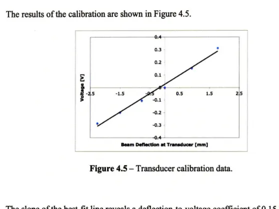
ation are shown in Figure 4.5.

0.4

Bem Deflection at Trunducer [mm]

Figure 4.5 - Transducer calibration data.

The slope of the best-fit line reveals a deflection-to-voltage coefficient of 0.15 V/mm. The inverse of the slope thus provides our desired voltage-to-deflection coefficient of 6.8

mm/V.

4.2.2 Measurement of Beam Stiffness

The beam stiffness, K, is defined as

Km- force displacement'

where, in the case of a cantilevered beam, both the applied force and measured displacement are at the free end. Because the position transducer does not measure displacement at the free end of the beam, the lengthfactor, see Eq. (7), will be used to compensate for the offset transducer position, resulting in the following equation for the experimentally determined value of K

K = deflection - to - force(z,) * lengthfactor(z,), (34

3)

I)

0.4

N. _:l9 I

F

The results of the calibr

2 5

(20)

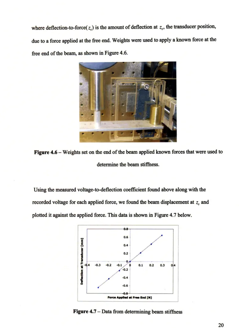
where deflection-to-force(z,) is the amount of deflection at z,, the transducer position, due to a force applied at the free end. Weights were used to apply a known force at the free end of the beam, as shown in Figure 4.6.

Figure 4.6 - Weights set on the end of the beam applied known forces that were used to determine the beam stiffness.

Using the measured voltage-to-deflection coefficient found above along with the recorded voltage for each applied force, we found the beam displacement at z, and plotted it against the applied force. This data is shown in Figure 4.7 below.

Force Appied at Free End [N]

Figure 4.7 - Data from determining beam stiffness

.4 -O

I

.4

(21)

The slope of the best-fit line thus gives the force-to-deflection(z,) value of 2.2 mm/N. Taking the inverse of this value and converting millimeters to meters yields our desired deflection-to-force(z,) value of 450 N/m. To now solve for K, we simply evaluate the lengthfactor(z,) to find that it equals 0.70, which, when inserted into Eq. (34) yields a beam stiffness of 320 N/m.

4.2.3 Measurement of Natural Frequency

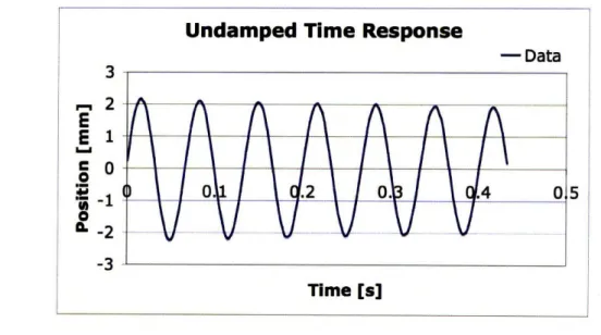
To obtain the natural frequency, co,, an impulse was given to the beam, which was allowed to vibrate freely with no damping. See Figure 4.8 below for the data.

Undamped

Time Response

3 2-- 2 El

o

0 .2 _0. _.4 ₀₅ I -2 Time [s]

Figure 4.8 - Undamped system response used to determine the natural frequency

Although a very small amount of damping results in a slight decay in successive peak amplitudes, it is small enough to disregard. Eq (16) was fit to this data, giving a natural frequency of 92.0 +/- 0.044 rad/sec with a 95% confidence interval.

(22)

4.2.4 Measurement of Magnetic Field

A bar magnet produces the magnetic field through the damping fluid and is mounted below the damper on a vertical linear stage. By turning the knob on the top of

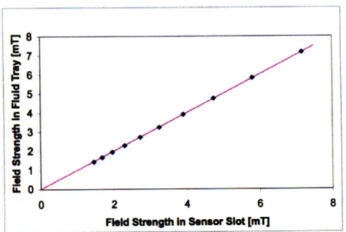
the stage, the magnetic field through the MR fluid is varied as the magnets are brought closer or further away from the fluid. The strength of the field is measured using a Vernier Gaussmeter that is inlaid in the plastic fluid tray the same depth as the fluid,

which allows it to measure the magnetic field through the same medium (distance of air and plastic) as the field that affects the fluid. Below, in Figure 4.9, is data showing the measured field in the fluid gap versus the measured field in the sensor slot for numerous magnet positions with a line of slope 1 drawn through them.

. . . .. . . . E. Y7-c 4 2 FUl tngth in S or Slot [m

Field Strength In Sensor Slot [ml)

Figure 4.9 - Plot comparing the measured magnetic field in two locations

Both sensor slot and fluid tray are located at equal distances from the edge of the magnet, so the edge effects detected at the sensor slot are approximately equal to the edge effects in the fluid tray. Based on the data in Figure 4.9, it will be assumed that the measured field in the sensor slot equals the field in the fluid tray.

I

_I

i

a a 6 il teghi esrSo [m8

(23)

4.2.5 Measurement of Damper and Gap Dimensions

The gap thickness, 6, was determined by placing a shim of a known thickness in the fluid trough and lowering the damper until it comes in contact with the shim, thus producing a 6 of the same thickness as the shim. The dimensions of the damper were also measured using calipers and mean values with 95% confidence intervals are shown for all three measurements in Figure 4.10.

95% confidence interval Mean [mm] [mm] Gap thickness 1.61 0.0080 Damper width 14.7 0.033 Damper length 47.2 0.021

Figure 4.10 - Gap thickness, damper length and width measurements.

4.2.6 Determination of Diffusion Time

Given a gap thickness of 1.61 +/- 0.008 mm, Eq. (26) can be used to find the diffusion time of the impact through the fluid, assuming the kinematic viscosity is known. However, the effective viscosity varies throughout the experiment as the

magnetic field through the fluid changes. To ensure the diffusive effects have propagated throughout the entire amount of fluid, the longest possible diffusion time is calculated for the given gap thickness. Recalling Eq. (26), the smallest value of v will result in the longest possible diffusion time, thus the minimum viscosity, No , is divided by the fluid density 3320 kg/mA2, which results in a diffusion time of 2.90 x 10^-4 s. When this time is compared to the period of oscillation, 1.1 x 10^-2 s, it can be assumed that all of the diffusive effects of the impulsive start have been diffused throughout the fluid for

(24)

essentially the entire period of oscillation. Thus, the impulsive start does not frustrate the above analysis.

4.3 Procedure

Recall the purpose of this experiment: to characterize MR fluid that will be used to model a variable shock system. One of the principal fluid properties that will be used in modeling a variable shock system is the fluid's yield stress, which greatly affects how it behaves as a shock absorber. Students will need to know how the yield stress varies with magnetic field. This relationship can be found by fitting Eq. (16) to the time response of an impulsively started vibrating beam at numerous magnet positions. The varying magnet positions result in a varying magnetic field through the MR fluid, which will be recorded by the magnetic field sensor. Because the natural frequency for the system has already been determined, extracting C from the fit equation becomes a matter of algebra. Once the damping ratio is obtained, Eq. (16) is used to determine the constant

C, which is then inserted into Eq. (32), along with physical parameters, to find the yield

stress of the fluid for a particular magnetic field strengths.

5. Results and Discussion

Below, in Figure 5.1, is a plot of the fluid yield stress versus magnetic field intensity. Magnetic field intensity is commonly used in the literature and thus the

measured magnetic field density, B, had to be converted to H. The max value of B in this experiment is less than 10 mT, which means a linear relationship between B and H can be used. See Figure 5.1 below for the B-H curve of MRF-336AG.

(25)

-81

H (hA/m)

Figure 5.1 - Plot of yield stress versus magnetic field intensity.

The experimentally determined yield stress versus magnetic field intensity is shown below in Figure 5.2, _{followed by the supplier provided information in Figure}_5.3.

(26)

10 CR °fý Uk 0 4h 5

H (kAmp/m)

Figure 5.2 - Plot of experimentally determined yield stress versus magnetic field intensity.

0 H (kA/m)

Figure 5.3 - _{Plot of supplier-provided yield stress versus magnetic field intensity.}

--·---

··-- ·---

···--·--r----~*- r

_i i 1 VI Q) k QS · rl

(27)

The most glaring difference between the data is that the scale ofH in the provided data is two orders of magnitude greater than the scale of the experimental data. However, given the precision of the magnetic field sensor and the provided relationship between B and H, the experimentally determined field intensity should not have such great error. The disparity of the data likely comes from the calculation of xd, in which initial damper

velocity was used to calculate the shear rate. The initial velocity is the greatest, because no damping has occurred yet. Thus, because the greatest possible shear rate was used, the

calculated yield stress should be higher than it actually is, which the data seems to suggest given the certainty of H.

Both data show relationships that are concave up in the corresponding ranges of H, though the experimental data has a steeper increase in yield strength as Hincreases. This artifact can be explained by using the initial damper velocity as a representative value. Figure 5.4 below shows the system response at both low and high magnetic field strengths.

* low field i high field

4 N -5 --- --- --- --- --- -- -- -- ----E3 9 - --L *a ;io 0-10. -2 -3 - _ _

-41-LTime

[s] _ Time [s]

Figure 5.4 - System response at 0.0654 kAmp/m (left) and 4.02 kAmp/m (right). Notice the increased amount of damping on the right.

E 2 E 9 ICo o ILI -3 . -4 1 '

(28)

Because of the rapid damping of the system at high magnetic field strengths, the initial velocity is less representative of the data than it is at low field strengths; specifically, it is a greater overestimation. Referring to Eq. (30), one can see that a higher damper velocity

results in a higher yield stress.

Although MR fluids are most often modeled as Bingham plastics when in the presence of a magnetic field, they are quite reasonably modeled as Newtonian fluids with no field. Because a relatively small magnetic field was used in this experiment, a

Newtonian model was also used to characterize the fluid to investigate how accurately it can characterize MR fluid at low field intensities. Figure 5.5 shows viscosity, as

determined using the Newtonian model discussed in section 3.3.1, plotted against magnetic field intensity.

4

3

0 1 2 3 4

H (kAmp/m)

Figure 5.5 - Using a Newtonian model, the viscosity is plotted against magnetic field strength. ++ ···9----+-·--··· ·-·-···-;··- ···- · + + + +i~ 1C - +i f+ + ... _...~..._~~i..+. ..._ ~1 _ ++

(29)

Close inspection of Figures 5.2 and 5.5 suggest that at such low field strengths, a Newtonian model describes the fluid behavior just as well as a Bingham plastic model.

This finding suggests that at low field strengths, students can model the MR fluid in the 2.672 variable shock experiment as a Newtonian fluid with a field-dependent viscosity.

6. Considerations for 2.672

6.1 Design Rationale

Because this experiment is designed for use in 2.672, special considerations were made in its design to allow for easy student interaction.

6.1.1 Open Access

The layout of the experiment, shown in Figure 6.1 below, was designed to allow students easy access to the interactive parts while hindering access to fixed components.

(30)

All of the interactive parts are on the right side of the setup, making them easily

accessible and their position more intuitive for the right-handed students, which are the majority. All other parts, which should not be adjusted by students, were positioned such

that students would have to go out of their way to loosen or adjust them. For example, the bolts on the beam clamp are facing away from students, the entire transducer support is in the back of the experiment, and all the bolts on the interactive right side that should not be adjusted are facing into the experiment and difficult to access.

6.1.2 Interchanging Fluid Tray

In 2.672, students are expected to test their models by varying numerous parameters. One parameter they can vary in this experiment is the fluid itself by

interchanging fluid trays. See Figure 6.2 for a picture of the tray platform and fluid tray.

(31)

To gain access to the trays, they simply loosen two bolts behind the linear stage. Which two bolts need to be loosened is intuitive because they are the only two that are readily accessible. See Figure 6.3.

Figure 6.3 - (left) Fluid platform in raised position with damper resting in fluid. (right) Platform lowered by loosening two bolts, allowing access to fluid trays

Once the platform is lowered, students unscrew the plastic wing-nuts and remove the plastic bolts, both shown in Figure 6.4, to interchange the fluid trays.

(32)

Figure 6.4 - Plastic wing nuts secure the fluid tray to the platform.

Plastic bolts and wing-nuts are used to not only hold the trays in place, but also tighten them to the platform to ensure a constant gap thickness for any of the trays. Plastic bolts

and wing-nuts were used to prevent students from over tightening a metal bolt which could lead to cracking in the plexiglass platform or tray. Furthermore, the plastic does not interfere with the magnetic field, which allows for a constant field through the fluid.

6.1.3 Fluid Tray Cover

Due to the schedule of 2.672, this experiment will often go days without being used. To prevent the MR fluid from drying out and free from dust or other floating

particles, a plastic cover has been incorporated into the design of the fluid platform. A plastic lid was obtained from the VWR stockroom and then a channel, into which the lid fits, was milled into the platform. See Figure 6.5 below to see the cover.

(33)

Figure 6.5 - Plastic cover to prevent drying out and contamination of fluid.

Students will simply lower the entire platform and place the cover in the channel when they are finished with the experiment to protect the MR fluid.

6.1.4 Transducer Alignment

The alignment of the transducer is crucial to obtaining good data, as the aluminum plunger should not touch the inside walls of the transducer while it vibrates. To allow for easy alignment of the transducer, all three dimensions of its position are adjustable, as shown in Figure 6.6.

(34)

The lateral motion of the transducer clamp is possible because of a channel that has been milled into the clamp support, as shown in Figure 6.7 below.

Figure 6.7 - Milled channels allow for lateral motion of the transducer clamp.

6.2 Maintaining Fluid Gap

When the damper is first lowered into the fluid tray containing the MR fluid, it will force out some fluid onto the sides of the damper. This excess fluid increases the contact area of the fluid and needs to be removed from the sides of the damper. See Figure 6.8 below to see the excess fluid.

(35)

The increased fluid contact area results in a higher than expected viscosity because the additional area is not accounted for. To remove the excess, simply excite the beam a few times until the sides of the damper no longer have fluid on them, as shown in Figure 6.9. The fluid will typically seep onto the edge of the tray as shown.

Figure 6.9 - _{Excess fluid has been removed from damper.}

If the excess is not removed from the damper before gathering data, the increased contact area will result in higher than expected viscosity, because the additional contact area is difficult to measure and incorporate into calculations. Assuming a constant contact area of the bottom of the damper, the measured viscosity versus the number of times the beam was excited are plotted below in Figure 6.10.

(36)

3.2 .?ý 3.1 W 0 rn U PI 0 2 4 6 8 Number of Excitations

Figure 6.10 - Data showing effect of excess fluid on damper.

Notice how the viscosity begins near 3.2 Pa*s, but settles around 3 Pa*s after a few excitations, from which the excess fluid on the damper is removed. Furthermore, the last data point shows how the fluid begins to thin out under the damper after 5-10 excitations. Such spreading also results in a different damping area than expected and produces bad data. See Figure 6.11 below to see what the thinly spread fluid looks like.

Figure 6.11 - Fluid spread too thinly after 5-10 excitations of beam.

9

9 0

9

(37)

Note how only a fraction of the left side of the damper is actually in contact with the fluid. Once the fluid is no longer in contact with the entire area of the damper, the platform must be lowered so the fluid can be re-spread before taking more data.

7. Future Work

Some future areas of work on this experiment include:

*: Designing a new damper that maintains a constant gap thickness for longer periods of

time. The current design requires the MR fluid to be reapplied after approximately 10 tests.

i If current design of damper is used, bolt it on to the beam instead of gluing it. Be sure

to design an adjustable tilt into how you fix the damper to the beam to ensure parallel plate flow between the damper and fluid tray.

+

Using the setup to investigate the rate dependence of viscosity. Explore how this dependence varies with magnetic field.

*.# Make fluid trays of varying pocket depth, which would allow students to vary the gap thickness.

• Obtain a better magnetic field sensor. The Vernier model used is intended for

educational purposes.

(38)

8. Nomenclature

A Coefficient of fit for free-vibration equation Ao Initial peak displacement of damper

C Damping constant in spring-mass-dashpot system Cp, Damping constant at plate

6 Gap thickness of fluid

6di Impulse diffusive layer thickness E Beam modulus of elasticity

F Force applied to point mass in spring-mass-dashpot system

FpB Shear force exerted on plate by Newtonian Fluid

FpN Shear force exerted on plate by Newtonian Fluid G Complex material modulus

y Shear rate

y Shear strain

Gain Static gain of system H Magnetic field strength

Hen (s) "Engineering" transfer function of system Hphys(s) "Physical" transfer function of system

I Beam moment of inertia

K Spring constant

1 Length of damper

L Beam length

M Point mass in spring-mass-dashpot system

# Viscosity

Po Viscosity of MR fluid in absence of magnetic field v Kinematic viscosity

Con Natural frequency of system

Phase angle s

tdif Impulse diffusion time

' Shear stress

v,, (H) Field-dependent yield stress u(y) Fluid velocity in damper

w Width of damper

x Position of point mass (plate)

XL Beam free-end deflection

xz Beam deflection at position z along beam

xpI Plate velocity

z Position along beam

z, Position of transducer along beam 5" Damping ratio

(39)

9. References

"Audi: Adui S3." Automotive Intelligence, 2004. Accessed on 03/13/08.

http://www.autointell.com/european companies/volkswagen/audi-ag/audi-cars/audi-s3/S3-suspension-system- 120mm.JPG

Bender, Jonathan W. , Carlson, J. D., and Jolly, Mark R., "Properties and Applications of Commercial Magnetorheological Fluids," SPIE 5th Annual Int Symposium on Smart Structures and Materials, San Diego, CA, March 15, 1998.

Carlson, J. D., Catanzarite, D. N., and St. Clair, K. A., "Commercial Magneto-Rheological Fluid Devices," Proceedings 5th Int. Conf on ER Fluids, MR Suspensions and Associated Technology, W. Bullough, Ed., World Scientific, Singapore (1996), 20-28.

Carlson, J. D. "What Makes a Good MR Fluid?," 8th International Conference on ER Fluids and MR Fluids Suspensions, Nice, July 9-13, 2001.

Cravalho, E., Smith, J., Brisson II, J., McKinley, G., 2.005 Thermal-Fluids Engineering Course Notes. Fall 2006.

Dimock, Glen A., Wereley, Norman M., Yoo, Jin-Hyeong. "Quasi-Steady Bingham Biplastic Analysis of Electrorheological and Magnetorheological Dampers" Journal ofIntelligent Material Systems and Structures 2002; 13; 549.

Hirani, H and Sukhwani, V K. Design, development, and performance evaluation of high-speed magnetorheological brakes. Department of Mechanical Engineering, Indian Institute of Technology. August 2007. DOI: 10. 1243/14644207JMDA120 Hughey, Barbara J. and Hunter, Ian W., "Electro-Mechanical System Experiment:

Background", 2.671 Laboratory Instructions, MIT, Fall, 2006 (unpublished). Kundu, Pijush, Fluid Mechanics. Academic Press, 1990

LORD MR Solutions, "Designing with MR Fluids," Engineering Note, December 1999. LORD MR Solutions, "What is the Difference between MR and ER Fluid?"

Presentation, May 2002.

LORD MR Solutions, "Permanent -Electromagnet System," Engineering Note, March 2002.

Lord, 2008, Lord Corporation MRF-36AG Product Information Sheet, (Lord Corp. OD DS7011 (Rev. 05/06)).

(40)

Appendix A

-

Detailed Part List

Part Supplier Supplier's Contact Info Part #

A Aluminum Clamp n/a n/a n/a

Macrobench - 4 hole adapter plate w/

B adjustable ring Linos www.linos.com G070001000

Macrobench - Support

C Rod, 90 mm Linos www.linos.com G070025000

Technical Clean Top II Honeycomb Manufacturing

D Optical Top Corporation www.techmfg.com 77-107-12R

Ceramic Bar Magnet, Master

E 3X2X0.195 Magnetics http://www.maqnetsource.com/ CB1952

Plexiglass Platform w/

F fluid tray n/a n/a n/a

G Linear Stage McMaster-Carr www.mcmaster.com 5236A16 Macrobench

-Connecting Clamp, 120

H mm Linos www.linos.com G070016000

I Magnetic Field Sensor Vernier www.vernier.com MG-BTA Macrobench - Cross

3 Clamp Linos www.linos.com

K Position Transducer Sentech Inc. www.sentechlvdt.com DCFS2 L Aluminum Beam McMaster-Carr www.mcmaster.com 89215K418

Development of laboratory class experiment to characterize magneto-rheological fluid