Determining Signal-to-Noise Ratio in a Burst Coherent
Demodulator
by
Janet Liu
Submitted to the Department of Electrical Engineering and Computer Science
in Partial Fulfillment of the Requirements for the Degrees of
Bachelor of Science in Electrical Engineering and Computer Science
and Master of Engineering in Electrical Engineering and Computer Science
at the Massachusetts Institute of Technology
May 1999
@1999
Janet Liu. All rights reserved.
The author hereby grants to M.I.T. permission to reproduce and
distribute publicly paper and electronic copies of this thesis
and to grant others the right to do so.
Author...
Department of Electrical Engineering and Computer Science
May 28, 1999
C ertified by ... . ... . . , .. ... . ... . s.... ...G. David Forney
Thesis SupervisorAccepted by...
-
... ...
. . .
Arthur C. Smith
Chairman, Department Committee on Graduate Theses
Determining Signal-to-Noise Ratio in a Burst Coherent Demodulator
by
Janet Liu
Submitted to the
Department of Electrical Engineering and Computer Science May 28, 1999
In Partial Fulfillment of the Requirements for the Degrees of Bachelor of Science in Electrical Engineering and Computer Science and Master of Engineering in Electrical Engineering and Computer Science
Abstract
Effective methods of performing diversity selection in wireless systems has been demon-strated to significantly reduce bit error rate. Information about the noise on a channel can allow accurate selection of the best diversity branch. This thesis, based on research conducted at Telcordia Technologies (formerly Bell Communications Research) describes a study of the PACS demodulator. The study was aimed at investigating possible meth-ods of estimating the signal-to-noise (SNR) ratio on a wireless channel. In the interest of maintaining the current system and of taking advantage of the primary features of the
PACS system, two quality metrics, based on the phase disturbance of the received signal,
were studied to determine their correlation to noise. A description of these metrics and their proposed relationship to noise is provided. Methods to analyze the performance and reliability of the metrics are described, along with a simulation environment for evaluating their performance. Finally, initial results of the analysis is presented, accompanied by a brief evaluation of these results.
Thesis Supervisor: G. David Forney
Acknowledgments
I wish to express my thanks to Rob Ziegler, my supervisor at Telcordia Technologies. Much of the work described in this thesis is due to the simulation efforts of the PACS system that he initiated. He offered me technical guidance and support and often went beyond the call of duty to assist me and to give me a positive experience during my time away from campus.
I would also like to thank Telcordia Technologies and the MIT VI-A Program for spon-soring this thesis and for providing me with an opportunity to do research in a corporate environment. I will always consider it a valuable part of my MIT education. Thank you to all the faculty who have taught me many new and exciting things in my five years here. They have also provided me with an irreplaceable education. Final thanks to my on-campus supervisor, Dr. G. David Forney, particularly for his editorial contributions to Section 2.2 of my thesis document.
I would like to thank my family for all they have done for me these years. My journey through MIT is as much their accomplishment as it is mine. Thank you for loving me and supporting me through the entire experience. I could not have done anything without them.
I would like to thank my friends, my church, and my fellowship who have been incredibly supportive and encouraging throughout this whole process. They have been my family here, and I appreciate the loving kindness they have never failed to show me. Special thanks for their many prayers and encouragements. It made all the difference.
To my family and friends: Your unconditional love has humbled and reminded me to focus on what is important. If I were to choose the one thing I learned the most from this experience, it would be how precious God's people are and how much I need everyone God has put into my life.
Lastly, and most importantly, I would like to thank my Father in heaven, and my Lord and Savior, Jesus Christ for His abundant grace and love. You give me life in full, and all blessings in abundance. I owe all of who I am and what I have to You. I pray this experience has been to Your glory.
Contents
1 Introduction 8
1.1 Personal Access Communications System (PACS) . . . . 9
1.2 Diversity Selection . . . . 9
2 Background: System Overview 11 2.1 M odulation . . . . 12
2.2 Square-Root-of-Raised-Cosine Nyquist Filtering . . . . 13
2.3 Bandpass-to-Phase . . . . 15
2.4 Symbol Timing . . . . 16
3 Objective: Estimating SNR on a Wireless Channel 18 3.1 O bjective . . . . 18
3.2 Experimental Models . . . . 19
3.2.1 Quality Metrics . . . . 21
3.3 Phase Jitter . . . . 25
3.3.1 Approximations to the Probability Distribution of the Phase Distur-bance ... .. ... 25
3.3.2 Expected Results . . . . 27
4 Experiments 30 4.1 Design of The Experiment . . . . 30
4.2 Hardware Simulations . . . . 31
4.2.1 Issues and Modifications to the Model . . . . 32
4.3 Establishing a Data Set . . . . 32
4.4.1 Deriving Distributions and Goodness-of-fit Testing . . . . 4.4.2 Discriminating Between SNR Levels . . . .
5 Results
5.1 QI ...
5.1.1 Goodness-of-Fit Testing . . . . 5.1.2 Ability to Discriminate Between SNR Levels . . . .
5.2 D P .. . . .
5.2.1 Goodness-of-fit Testing . . . . 5.2.2 Ability to Discriminate Between SNR Levels . . . .
5.3 SNR Discrimination . . . .
6 Conclusion
6.1 Summary ...
6.2 Future Work . . . . 6.2.1 Possible Numerical Methods. 6.2.2 Possible Analytical Methods 6.3 Concluding Remarks . . . . A Simulation Code References 33 35 36 36 38 39 40 41 42 42 49 49 50 50 51 52 53 59
List of Figures
2-1 Block Diagram of PACS Demodulator . . . . 11
2-2 Phase Constellation for i-shifted QPSK . . . . 12 2-3 Block Diagram of Bandpass-to-Phase portion of the Circuit . . . . 15 2-4 An eye-diagram: the sampling point that produces the largest eye-opening
is the one closest to the correct sampling phase. . . . . 17
3-1 (a) Ideal Phases: Vectors line up perfectly. (b) When the individual phases vary, the resultant vector has a phase that is the "average" of the composite phases. . . . . 23 3-2 Differential Phase - measure the deviation from the ideal AO = 0 . . . . 24
3-3 Probability density of p(O) for y = 1, 5, 15, 20 dB . . . . 26
3-4 Probability density of p(O) of phase error 0 due to additive noise and its approximation function (0,'-) . . . . 27
4-1 Plot of Mean QI and Mean DP Values over SNR levels from OdB to 30dB 33
4-2 Sample Histograms of QI (a) and DP (b) samples at SNR = 15 dB . . . . . 34
5-1 Plot of Mean QI Values and its Standard Deviation over SNR levels from
OdB to 30dB ... .. ... 37
5-2 (a) Mean QI vs. E[QI] (b) Calculated vs. Derived Variance of QI The solid
line represents the measured means and variances of QI's for 1000 different simulations at SNR levels 10dB and higher. The dotted lines are the curves given by Equation 3.7 and Equation 3.8. . . . . 38 5-3 Mean QI values with Error Bars to indicate plus or minus one Standard
D eviation . . . . 39 5-4 Sample Distances Between Distinguishable SNR levels for QI metric . . . . 44
5-5 Plot of Mean DP Values and its Variance over SNR levels from OdB to 30dB 45 5-6 The solid line represents the calculated means and variances of DP's for 1000
different simulations at SNR levels 10dB and higher. The dotted lines are the curves given by Equation 3.9 and Equation 3.10. (a) Mean DP vs. E[DP] (b) Calculated vs. Derived Variance of DP . . . . 45 5-7 Second-order statistics of QI versus DP. . . . . 46
5-8 Sample Distribution of 1000 DP data points at 15dB SNR. . . . . 47
5-9 Mean QI values with Error Bars to indicate plus or minus one Standard D eviation . . . . 47 5-10 Sample Distances Between Distinguishable SNR levels for QI metric . . . . 48
Chapter 1
Introduction
In the past decade, the demand for commercial mobile communications has risen dramati-cally. Implicit in the demand for wireless communication is the need for highly reliable and affordable service, equally accessible from a variety of environments: urban, suburban, and rural; indoor and outdoor. In response to these demands, the telecommunications industry has developed several standards designed to specify delivery of these services to the various types of regions.
Two types of cellular service have been developed to meet the needs of an increasingly mobile society: high-tier and low-tier cellular service. High-tier cellular is characterized by high-power transmitters and macro-cell coverage and is designed for subscribers moving at vehicular speeds. Low-tier systems feature low-power transmitters and micro-cell coverage and provide the complementary service to subscribers moving at pedestrian speeds.
There are several high-tier and low-tier standards in place globally. GSM, TDMA, and CDMA are the common high-tier standards in Europe and North America. They have met with considerable success in their respective regions of operation. Low-tier standards have been less widely deployed in the U.S., although the Personal Handyphone System (PHS) has been well accepted in Japan. Two other low-tier standards, Digital European Cordless Telecommunications (DECT) and Cordless Telephone second generation (CT2), have formed the basis for private branch exchange (PBX) products [1].
One final standard, developed in the U.S., is Personal Access Communications Sys-tem (PACS). A significant portion of the PACS development work was done at Telcordia Technologies (formerly Bell Communications Research), and some unique technology has
emerged relating to this standard. Currently, there is extensive work being done to develop a PACS handset, which boasts a low-overhead burst coherent demodulator and a design that takes advantage of many of the features of the PACS standard. Development work in this area is continuing to expand to include not only the hand-held device, but also a full-service wireless local loop and a third-generation wireless system with wireless LANs.
1.1
Personal Access Communications System (PACS)
PACS is an ANSI standard for 1900 MHz low-tier Personal Communications Systems (PCS) service. It is characterized by micro-cell coverage, low transmit power, and low complexity, and is ideal for neighborhood applications, such as indoor wireless, wireless local loop, and pedestrian venues. It offers several advantages over macro-cell systems. For instance, PACS equipment is simpler and less costly and operates with a lower delay, and yet is more robust than indoor systems. Moreover, PACS has demonstrated satisfactory operability under high-speed vehicular mobility conditions and is well-suited to deliver high capacity, superior voice quality and ISDN data services. Therefore, PACS is a viable solution to providing high user density in both indoor and outdoor environments [2].
PACS technology is being developed because it can be combined ideally with the tra-ditional high-tier services, already in widespread use, for complete wireless service. PACS is able to provide virtually land-line quality service using radio ports that are simple and low-cost. With such an affordable and reliable low-tier standard, wireless technology could easily become a viable alternative to traditional land-line phones. In particular, countries with under-developed telephone switching systems could avoid costly installations of miles of wires and switching centers.
Given this motivation for developing PACS technology, providing the best quality at the fastest rate is a major goal.
1.2
Diversity Selection
In wireless environments, diversity selection becomes an important issue. The ability to increase the quality of a received signal is essential. There are many techniques that can be used to achieve this goal. Increasing the power of the transmitted signal, and thereby increasing the signal-to-noise ratio (SNR), is one approach. In a typical additive white
Gaussian noise channel, this method is quite effective in its ability to decrease the bit error rate of the signal. However, practical constraints prevent wireless hand-held systems from transmitting signals with unlimited power. Therefore, additional methods effective in reducing error rate must be employed in combination with higher transmit power. For instance, in a typical multipath fading channel environment, diversity selection has been shown to improve SNR more efficiently than higher transmit power or additional bandwidth
[1].
In particular, branch diversity selection is often employed to mitigate the effects of Rayleigh fading. This type of branch selection can be made on the basis of the best signal-to-noise ratio. Therefore, being able to accurately estimate the SNR on a given channel is central to this selection method and to the quality of the received signal [3]. Devel-oping effective methods of diversity selection is crucial to the performance of a wireless communications system.
We are therefore motivated to study methods that can improve diversity selection. We describe an efficient method that is easily incorporated into the overall system. Minimizing additional hardware and computational complexity are major constraints on the overall goal of improving diversity selection. However, the PACS demodulation algorithm offers several key features which can be exploited and used to estimate the SNR on a given channel and ultimately to aid in diversity selection. This thesis studies the demodulation algorithm, its unique features, and the design of the hardware system and presents results that may offer insight into developing future methods of diversity selection based on symbol timing.
The following chapters will discuss various aspects of the project and the methods investigated. Chapter 2 describes the PACS system and establishes the background for the research described in the following chapters. Chapter 3 states the objective of the thesis and provides a theoretical discussion of the principles underlying our study. Chapter 4 is an overview of the design of the models used in the simulations and experiments. Chapter
5 describes the simulation and analysis systems applied to the data in order to provide
a measure of the metrics' ability to accurately estimate SNR and states the results from these simulations. Finally, Chapter 6 summarizes the overall conclusions from this study, including recommendations for future work, and gives the author's perspective on further research and development in this area.
Chapter 2
Background: System Overview
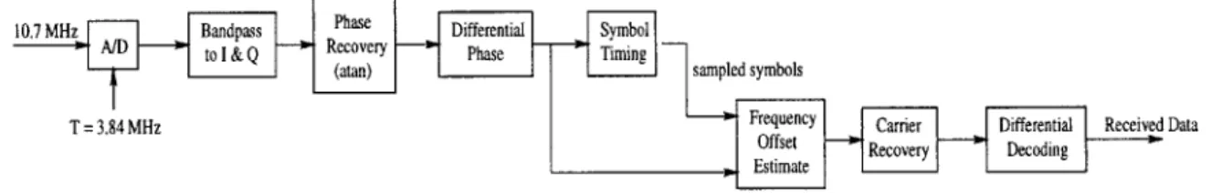
This chapter presents an overview of the pertinent elements of the PACS system design. A block diagram of the stages of the demodulation process is shown in Figure 2-1. The 10.7 MHz Bandpass Pae Differential _ Smo
i22 AID to I & Q ' Rcvry Phase Tmn
(atan) sampled symbols
T=3.84MHz Frequency Carrier Differential Received Data
Estmte -fRecovery Decoding
Figure 2-1: Block Diagram of PACS Demodulator
initial portion of the demodulation, in which the baseband signal is converted into phase information, also plays a crucial role and will be discussed in detail. Following this bandpass-to-phase portion, the demodulator circuit is then divided into several stages: symbol timing and frequency estimation, coherent carrier recovery, and differential decoding.
One of the primary motivations for this study is to improve the performance of current diversity selection techniques. It is desirable to be able to choose a diversity branch early in the demodulation process, and consequently, the majority of the research will focus on the bandpass-to-phase portion of the circuit, which precedes the decoding of the signal. Specifically, the symbol timing and frequency estimation portion of the demodulation circuit will be the primary focus of this study because many of the intermediate values computed to perform symbol timing contain information that is correlated with the noise and interference in the signal and will therefore consider many of the same noise issues relevant to diversity selection.
2.1
Modulation
There are a number of issues involved in choosing a modulation technique for wireless communication. For instance, some of the considerations include intersymbol interference, spectral efficiency, power spectral efficiency, and out of band power. Quadrature phase shift keying (QPSK) modulation is often preferred for its greater spectral efficiency. Furthermore, phase modulation, in general, provides an advantage since amplitude information is more vulnerable to the fading environments typical of wireless communication systems. The PACS system uses
}-shifted
QPSK.QPSK is a form of quadrature amplitude modulation (QAM), where the transmitted symbol at time i is zi = e6i', where the phase variable O takes on one of four equally-spaced phase values. In 7r/4-shifted QPSK, the set of possible phase values shifts by r/4 at every time i. In this manner, there is a guaranteed phase change between adjacent symbols, and the differential phase
Aoi = 62 - Oi-1
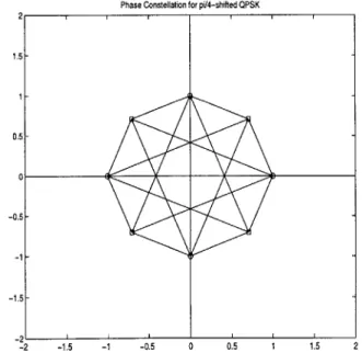
is always equal to an odd multiple of 7r/4. In fact, this characteristic will be a significant feature in the symbol timing circuit design and also in the method being described in this thesis. Figure 2-2 illustrates the phase constellations of this particular modulation scheme and the possible phase transitions between two adjacent symbols.
Phase Constellation for pil4-shifted QPSK
z~~ II I .5 -1 - - ).5--1 -1.5 -Fiu -1e 5 h05 -1 -0P5 1 1.5
Furthermore, a i-shifted QPSK modulation scheme offers several other design advan-tages for wireless systems. For instance, it provides the spectral efficiency of QPSK systems but with reduced amplitude fluctuations. Furthermore, not only does this method guarantee phase changes with every symbol, it also avoids phase changes through the complex origin. Zero-crossings require power amplifiers to maintain linearity across a wide-amplitude range
[5].
2.2
Square-Root-of-Raised- Cosine Nyquist Filtering
The data stream generated by the modulation must then be conveyed as the amplitude values of a signaling pulse shape, g(t). The design of the pulse shaping signal is determined by several constraints placed on its performance. The pulse shape should both minimize intersymbol interference (ISI) and also make the most efficient use of the spectrum of a band-limited channel. The PACS systems uses a square-root-of-raised-cosine transmit and receive filters, or pulse shaping signals. It has been shown in [6] that a square-root of raised-cosine pulse-shaping filter is the optimal choice for both the transmit and receive filters for minimal ISI and maximum SNR.
Using this method, the symbol sequence {zi} is modulated by quadrature amplitude modulation (QAM) using a squaroot-of-raised-cosine transmit filter with impulse re-sponse g(t). The transmit signal is
s(t) = R{x(t)ejwt} = Xr(t) cos(wt) - xi(t) sin(wt),
where Xr(t) and xi(t) are the real and imaginary parts of the complex signal
x(t) =zig(t - iT),
{zi} is the complex ir/4-shifted QPSK symbol sequence, g(t) is a real
square-root-of-raised-cosine impulse response, T is the symbol interval in sec, and w is the carrier frequency in radians/sec.
model. The received signal is simply
r(t) = s(t) + n(t),
where n(t) is AWGN with one-sided power spectral density No.
The receiver is a QAM demodulator using a matched square-root-of-raised-cosine receive filter g(t). After demodulation to baseband, the received signal is the complex signal
r'(t) = ejoax(t) + n'(t),
where n'(t) is still AWGN with one-sided power spectral density No, and 60 is a phase offset due to incorrect phase and/or frequency of the demodulating carrier. (It turns out that in a differential-phase-modulated system the phase offset may be ignored.) The baseband signal is then filtered in the receive filter and sampled every T sec.
The sample sequence ri is given by
ri = Jr'(t)g(iT - t) dt.
Because g(t) is real and even, this is equivalent to
ri =
J
r'(t)g(t - iT) dt;Note that because a square-root-of-raised-cosine filter is square-root-of-Nyquist, the T-shifted filter responses {g(t - iT)} are orthonormal; therefore
ri = ejo
zi +
ni,where x is the transmitted symbol and {ni} is an i.i.d. Gaussian sequence with variance U2 = No/2 per dimension.
In other words, there is no intersymbol interference and the phase offset 60 comes through coherently.
2.3
Bandpass-to-Phase
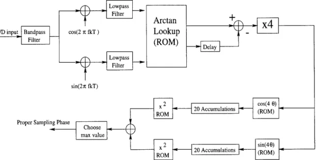
The bandpass-to-phase portion of the circuit will be emphasized because the majority of the methods developed in this study will take place in this particular sub-system. From Figure 2-1, this is the portion that receives the transmitted signal as its input and precedes the decoding of the signal. A more detailed block diagram of the bandpass-to-phase portion of the circuit is provided in Figure 2-3.
Lowpass] Filter
Arctan
+
A/D input Bandpass cos(2 n fkT )Lookup -
4
3WFilter
(ROM)
Dea Lowpass] Filter sin(21c fkT) x +- 20 Accumulations c(OM) ROM R4M)Proper Sampling Phase
mahovalue
x 2 -- 20 Accumulations i(OM) ROM(RM
Figure 2-3: Block Diagram of Bandpass-to-Phase portion of the Circuit
The PACS demodulation algorithm begins with the received continuous signal at an intermediate frequency of 10.7 MHz. An A/D converter digitizes this signal with a sampling rate of 3.84 MHz. Because the signal contains frequency components greater than the Nyquist rate, the sampling causes aliasing in the signal. The resulting sampled signal appears to be at 820 kHz. Sampling at this smaller frequency can be thought of as down-conversion using the third harmonic of the sampling frequency, which in effect is a high-side injection with an associated phase inversion.
At this point, although the signal is at 820 kHz, the remainder of the circuit is clocked at 960 kHz, resulting in a bulk frequency offset of 140 kHz. This offset is a compromise resulting from a series of filter design decisions that sought to optimize the filter coefficients to eliminate the need for multipliers in the digital circuit.1 The performance degradation
this offset causes is negligible and has been confirmed by experiment to be acceptable, and as shown in Section 2.2, this constant phase offset has no effect on the remaining analysis. The digitized signal is then passed through a bandpass filter to suppress DC compo-nents and quantization noise outside the desired passband [2]. The filtered signal is digitally mixed with sine and cosine carriers at 960 kHz, and two low-pass filters eliminate the double-frequency components of the in-phase and quadrature (I and
Q)
components of the received signal. Using an arctangent function, the I andQ
components are translated into phase information. The difference of the phases of consecutive symbols is taken to obtain the differential phase. Recall that the !-shifted QPSK modulation scheme employed by the transmitter ensures that the difference between the phase of two consecutive received sym-bols is one of four differential phases, t} or ± . The differential phase is then quadrupled to remove modulation [2]. This quadrupled differential phase is passed to the remainder of the demodulating circuit.2.4
Symbol Timing
The symbol timing stage of the circuit plays a critical role in this study. The need for symbol timing is a result of the fact that the incoming signal is 20x over-sampled and may experience an unknown delay in transmission. It becomes necessary to choose the correct sampling phase in order to demodulate the signal reliably. Once the symbol timing portion of the system has established the proper sampling phase, every twentieth sample is sent to the remainder of the system to be demodulated.
Symbol timing is achieved by comparing a quality metric that indicates the maximum average opening of the eye-pattern of the signal at each sample phase; the phase with the "best" metric is chosen as the proper sampling phase. Figure 2-4 demonstrates what is meant by average eye opening. When the signal is sampled at the incorrect phase, the eye diagram will reveal an increasingly smaller opening, corresponding to signal distortion due to ISI. However, at the correct sampling phase, the eye diagram should reflect the clear separation of the I and the
Q
rails. This corresponds to the ideal sampling phase.This method of selecting the proper sampling phase has demonstrated high performance.
that clock from standard crystal oscillators. 960 kHz is precisely one fourth of the sampling frequency. This makes it easy to divide the sampling clock to use for the remainder of the circuit.
2-
0-
-2-0 2 4 6 8 10 12 14 16 18 20
Figure 2-4: An eye-diagram: the sampling point that produces the largest eye-opening is the one closest to the correct sampling phase.
This suggests that this quality metric, or a similar one, may be used to indicate the quality of the overall signal as well. While the eye separation is an indication of the amount of ISI (minimal ISI indicates proper sampling phase) distorting the signal, any type of noise can also distort this eye opening and degrade the system's ability to achieve accurate symbol timing. Therefore, the quality metric used for symbol timing also inherently includes the effects of other types of noise. This suggests that this metric may be useful in performing diversity selection in addition to symbol timing. The desire to increase the efficiency of the circuit by extracting additional performance from the current hardware and design provides sufficient motivation to pursue this possibility.
Chapter 3
Objective: Estimating SNR on a
Wireless Channel
We want to develop effective methods to compare the different noise levels of two wireless channels. There are two types of comparisons that will be useful. One is a relative compari-son of the noise levels of the two channels for purposes of diversity selection. It is important to the quality of the signal to receive it over the channel with the least amount of noise and interference. However, it is also useful to estimate the absolute level of the noise of a given channel. The PACS standard specifically states that the phone demodulator must be able to estimate within t3 dB the actual SNR level in the channel over which it is receiving the signal. It is certainly desirable to be able to guarantee a certain level of quality of service. For instance if a call cannot be received over a channel with a minimum SNR level, it should be dropped in order to maximize the system's resources.
3.1
Objective
One of the primary components of the PACS system is the demodulating algorithm. Data is modulated onto a carrier using '-shifted QPSK modulation with Nyquist square-root of raised-cosine spectral shaping. The data is then recovered using a low-overhead burst-coherent demodulation technique. The demodulator has several functions that contribute to the demodulation. A full description of the system can be found in Chapter 2. Once again, a key advantage of this implementation is the joint estimation of the symbol timing phase and the carrier frequency offset, described in Section 2.4. The demodulator also
employs a diversity selection technique that is based on a quality measure derived as part of the symbol timing/frequency offset estimation process.
Performing diversity selection as a "consequence" of the symbol timing/frequency off-set estimation process provides an efficient manner of increasing the performance of the algorithm; furthermore, simulations have shown that this technique presents performance advantages over the traditional method of diversity selection based on power and is almost as effective as diversity selection after channel decoding [1]. The method is founded on the premise that a channel quality metric derived as part of the algorithm can indicate the
"noisiness" of the channel.
The effectiveness of this method has been verified in both simulations and laboratory hardware experiments. However, while the utility of this method has been confirmed, its accuracy has not been adequately determined. Also, only its effectiveness as an indicator of relative SNR levels between diversity branches or different symbol timing candidates has been demonstrated; it has not been shown to explicitly convey information about the absolute level of SNR. Establishing a method of quantitatively estimating SNR in the chan-nel can provide improvements in both physical-layer signal processing and higher-layer link management protocols that rely on physical-layer measurements.
The aim of this thesis is to establish the reliability of the quality metric as an indicator of SNR in a channel and to determine its ability to convey specific information about SNR levels. Clearly, part of the objective includes selecting the least noisy channel without incurring heavy costs in terms of additional hardware or computational complexity. In order to optimize efficiency, emphasis has been placed on seeking methods that might be able to incorporate the channel selection method into the demodulation by establishing a clear relationship between SNR and a quantity derived from the demodulation process.
3.2
Experimental Models
All simulations and conclusions in this thesis will assume an additive white Gaussian noise channel model. This is simulated by adding complex Gaussian noise the input signal. That is, we let the noise, n = x + iy, where x and y are independent, identically distributed
Gaussian random variables. The variance, o = , of x and y is determined by the
SNR
Gaussian noise is added to the transmitted signal and undergoes the same treatment at the receiver end as the actual signal. The goal of this study is to characterize the effects of this
additive noise on the signal.
Once the channel is characterized and the behavior of the hardware can be simulated effectively, then it remains to establish several metrics which will indicate the "quality" of the signal. Our hope is that the signal quality will be directly related to the channel noise. This is a reasonable expectation, since noise clearly degrades the signal. However, it is important to note that noise may not be the only factor that affects signal quality. In this study, it will be assumed that these other effects are either negligible or independent of the channel noise.
If the noise level can be correlated to the value of a metric, a form of statistical estimation based on the metric can be established and become the basis of symbol timing selection, diversity selection, and frequency channel selection and link maintenance. This study will focus on determining if a metric can be developed that is useful for diversity selection. If its utility in this respect can be shown, it will be assumed, but not explicitly shown, that it can also be adopted to perform these other functions.
As described in Section 2.4, the current quality metric is derived from the in-phase and quadrature components of the transmitted differential phase. This is a likely candidate because it represents the phase information that is central to the demodulation algorithm and can be integrated easily into the demodulation process. It also effectively indicates the average eye opening of the eye-pattern of a burst. Furthermore, if the effectiveness of this metric can be determined, it may be possible to derive alternative metrics which may offer greater precision or accuracy.
The following subsections will offer a discussion on the derivation of the metric based on the in-phase and quadrature components and will provide an explanation as to why this metric presents itself as a reasonable indicator of noise. The introduction of an alternative metric will also be made with a brief comparison of the two. A more vigorous comparison will be given during the analysis and results sections.
3.2.1
Quality Metrics
Ideally, with no noise present and zero frequency offset from any source, the received dif-ferential phase multiplied by four yields t7r or ±37r, all of which collapse to ir. That is,
A6O = 4(6i - Oi-1) = (3.1)
Therefore, the quadrupled differential phase provides an absolute ideal phase value, 7r. Furthermore, the in-phase component is at its maximum magnitude of 1, and there is no
quadrature component.
Noise and residual and bulk frequency offsets cause the actual value to deviate from the ideal. Recall, the system undergoes a bulk frequency offset of 140 kHz, causing the ideal phase to actually be: AO = 7r - 4 - 2r -foff - T, where ff f represents the bulk frequency offset of 140 kHz and T = 3.84 MHz, the sampling period.
Any additional deviation can be thought of as representing the various forms of impair-ments experienced by the system, such as noise and intersymbol interference. The greater the noise level, the larger the deviation from the ideal. Assuming an ideal sampling phase and minimal ISI, the deviations represent only noise and interference other than ISI. How-ever, the deviation of a single symbol does not provide a precise measure of the noise level because noise and interference may introduce random errors at any sampling phase. Rather, it is more accurate to use a block of symbols and to average the error over this block in order to average out these random errors. Assuming that the channel conditions do not vary widely over the length of one burst (60 symbols), a burst can be used as a block of symbols. By accumulating over the center N symbols of a burst, we avoid symbols from the beginning and the end of each burst which may be affected by the signal ramping up or ramping down due to the filtering. With a sufficiently large N, where we take N to be the 47 center symbols in a burst, the "signal-to-impairment" ratio is maximized at the ideal sampling phase [3].
Note that although this discussion has included the effects of the bulk frequency offset, in reality the analysis that follows is unaffected by this additional bias. Compensating for this bulk offset so that we still deal with an ideal differential phase of 7r simplifies the analysis and has no bearing on the noise since the effects of the random noise and this bulk offset are separable. Similarly, we can also subtract this bias of -x, so that what remains
is a zero-mean variable. For this reason, the remainder of the discussions will refer to an ideal quadrupled differential phase A#, whose ideal value is zero, referring to an unbiased version of the differential phase, where
Aoi = 4(O6 - i - 1) - 7r. (3.2)
Each A/i is a zero-mean Gaussian with variance 16on where non-adjacent A#'s are in-dependent. However, adjacent phases are in-dependent. For example, Ai is correlated with both Aoi_1 and Aqi+1 but independent of any Aq# for any
j
5 i - 1, i, ori + 1.QI
The actual metric, called "Q", is derived from the in-phase and the quadrature components (the I and the
Q)
of the phase. Specifically, it is the sum of the in-phase components squared, added to the sum of the quadrature components squared,N N
QI
=
(E
sin(Ai
))2 +(E
cos(Aoj)) 2
(3.3)
i=1 i=1
which is effectively the squared magnitude of the sum of the N symbols. The QI essentially represents the cumulative magnitude of the phase deviation and can indicate the "signal-to-impairment" ratio. The phase of this resultant vector should approximate the average of the N individual differential phases.
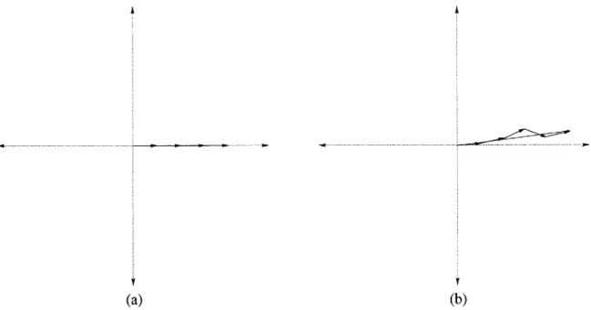
Summing a block of unit length vectors with an ideal phase, AO = 0 would yield a larger vector pointing in the same direction. This is illustrated in Figure 3-1 (a). However, noise and residual frequency offset due to differences in the carrier frequency references between the transmitter and the receiver cause the phases to fluctuate around the "ideal" phase so that AO' = 0
noise + Ooff, where 0
noise and 9
off represent random errors. Now,
instead of N angles all equal to A#, there is a set of angles {AO1,
#'2,
--- , AOM}, where the elements are uncorrelated random variables. However, the resultant vector sum over a block of N symbols could be viewed as approximating the "average" of these vectors, asshown in Figure 3-1 (b).
The sampling phase with the largest magnitude would signal the most accurate phase. Indeed, it has been observed and demonstrated in simulations, that there is an increasing
I
(a) (b)
Figure 3-1: (a) Ideal Phases: Vectors line up perfectly. (b) When the individual phases vary, the resultant vector has a phase that is the "average" of the composite phases.
monotonic relationship between SNR and the magnitude of QI. This result suggests that some significant relationship may exist between the two factors, and that the QI may be used as an estimator of SNR level. However, as the SNR becomes large, this best QI will approach a fixed value of N, so QI may not be a very sensitive indicator of SNR when the SNR is large. We will therefore investigate another quality metric which may be a more sensitive indicator of SNR.
Differential Phase
It may also be possible to reveal a useful correlation between SNR and the differential phase error itself. Ideally, the quadrupled phases will always wrap around to ir . Any deviation from 7r will be due to channel noise, ISI, or quantization noise. ISI and quantization noise are negligible at the correct sampling phase and can be ignored for the present time, although it is important to note that their contribution may still be non-trivial. A second metric, the differential phase error (DP), can be defined as variance of the deviation of the quadrupled differential phase from 7r.
N
The smallest error indicates the phase closest to the correct sampling phase. An illustration of the differential phase variance is given in Figure 3.2.1.
Figure 3-2: Differential Phase - measure the deviation from the ideal A#= 0
QI and DP are similar since the QI represents the two rectangular coordinates of the differential phase. The relationship between differential phase and SNR resembles the one described above for QI; in fact, it is the inverse. Therefore, it appears reasonable to compare the performance of these two metrics. They have a similar relationship to SNR and represent similar information in two different forms. QI is already in place as a quality metric in the current design of the demodulator; however, if DP is shown to offer performance advantages, the additional computation will be minimal, particularly since the calculation of QI and the calculation of DP have significant overlap.
In fact, there is reason to believe that DP may be a better measure of the noise. As SNR levels get larger, the ability of the QI metric to distinguish between levels weakens. The averaging effects of the vector summation will cause some loss of sensitivity. At close SNR levels, a direct representation of the differential phase itself may be able to yield finer distinctions.
3.3
Phase Jitter
Both QI and DP are dependent on the amount the differential phase of two adjacent symbols deviates from some "ideal" phase. This deviation of the quadrupled differential phase from ir is called the "phase jitter" and can be considered to be due to perturbations in the system. Specifically, DP measures the variance of that "jitter". The mean of DP is expected to be zero, that is zero "jitter" from the ideal phase. The smaller the variance, the less disturbance the signal is assumed to undergo. Similarly, QI measures the projection of the phase angle onto the real axis. Therefore, larger values of QI indicate a phase closer to the ideal phase, or small "jitter", and corresponds to lower noise levels.
Given these relationships, it is clearly advantageous to be able to approximate what the expected variations will be. These calculations will confirm the real data collected through the modeled channel. If the two sets of data do match, that will verify the model and also provide a means on which to base an estimation technique to determine the noise levels.
3.3.1 Approximations to the Probability Distribution of the Phase Dis-turbance
The detection method being developed in this study is based purely on signal phase informa-tion and employs maximum likelihood detecinforma-tion based on the signal phase in the presence of noise. The model approximates the combined effects of ISI, noise, and interference as a Gaussian process and aims to measure the phase disturbance of the signal due to different levels of interference. It is known that such a phase disturbance of a received waveform in complex Gaussian noise has a probability density function (pdf) given by:
1- 1O -0os 22
p(0) = re (1 + 1ry cose cos20 1)Je 2 dx) (3.5)
SNR
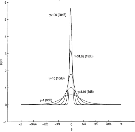
where -y is the SNR per symbol ( = = 10 10 ) [7]. Figure 3-3 displays p(O) for several values of -y. Clearly, as -y increases, corresponding to increasing SNR, p(O) becomes narrower and more peaked about 0 = 0. This represents a phase "jitter" that approaches zero as SNR increases. This also corresponds to the discussion above, where the variance of DP,
around its mean of zero, decreases as SNR increases.
Probability Distribution of Phase Jitter 6 7100 (20dB) 5- 4- 3-y=31.62 (15dB) 0. 2-r=10 (10dB) 1 y=3.16 (5dB) y=1 (OdB) 0 -1 -11 -37r/4 -ir/2 -7r/4 0 i/4 7/2 3/4 7 0
Figure 3-3: Probability density of p(9) for -y = 1, 5, 15, 20 dB
difficult to manipulate in calculations. However, we can see that when SNR is large and 0 is small, 9 is approximately just the quadrature noise component, which is a Gaussian variable
of mean zero and variance 1. Figure 3-4 illustrates that p(6) is well approximated by a
zero-mean Gaussian with variance 2n for SNR values of 10 dB and higher. The analysis in the following section will evaluate how QI and DP are expected to be affected by noise given by this approximation in the specified range of SNR levels.
2.5 2 15dB 1.5 10dB 5 dB 0.5-1 dB 0
-pi -3pi/4 -pi/2 -pi/4 0 pi/4 pi2 3pi/4 pi
Figure 3-4: Probability density of p(O) of phase error 0 due to additive noise and its ap-proximation function K(0,')
3.3.2 Expected Results
Based on the Gaussian noise-ISI-interference approximation model, it is possible to derive a set of expected results for both QI and DP. Recall that QI is defined as
N N
QI
=(Z sin(Aoi))
2+
(1cos(A0,))
2i=1 i=1
where each Aoi = 4(6i - Oi-1) - 7r and Oji and 0
i2 each has a probability distribution as
given in Equation 3.5. For higher SNR levels, it has been shown that 0, the deviation of the phase from the ideal is small and has a distribution that approximates a zero-mean Gaussian with variance Z. Consequently, Ai, being the scaled sum of two Gaussian ran-dom variables, is also another Gaussian ranran-dom variable with mean zero and variance 16o0.
Furthermore, because A# is expected to be small for higher levels of SNR, sin(Aosmaui) can be approximated as /\smau and cos(Aqsmaui) can be approximated as (1 - A"). This yields the following approximation for QI, given and SNR level greater than 10dB:
N N A0 2
Q
A)
2+ (Z
(1 - i ))2. (3.6)i=1 i=1
QI can be viewed as a random variable, and the calculations of both its mean and its variance can be greatly simplified using the approximations derived above.
From Equation 3.6, the expected value of QI (E[QI]) is
N N Ao2
E[QI] = E[(Z Aq,) 2 + (1(1 - %)2]
i=1 i=1
= N2
- (N2 - 1)(16U) + 1(N2 + 3N - 1)(16U) 2 (3.7)
and the variance of QI is given by
var(QI) = E[(QI)2] - E2[QI]
= (3N3 + N+ N - 4)(16un)2+ (-5N3 - 23N2 + 11N + 20)(1622)3 1 + -(9N 3 + 82N2 + 99N - 208)(16 n)4 16 (3.8)
The second-order statistics for DP follow a similar derivation. Recall,
N
DP =
Z(A~i
-Once again, A# is zero-mean Gaussian; therefore, DP =
Z'
1 Ao? and E[DP] can be given asN
E[DP] = E[Z Ao?]
and the variance of DP is given by
var(DP) = E[(DP)2] - E2[DP]
N
=
E[(Z A02)2] - (16No-2) 2 i=1= (3N - 1)(16o-2)2 (3.10)
These are the expected results for QI and DP. It will be demonstrated in Chapter 5 that these match closely with the actual results, within this range of interference, confirming the Gaussian approximation to Equation 3.5. Using these values, it is possible to detect maximum likelihood SNR level present in the channel, for SNR levels of 10 dB and higher. Unfortunately, similar results for smaller SNR levels is not available.
Chapter 4
Experiments
Quantitative data can confirm the theoretical results developed in Chapter 3. For the purposes of analysis, it is preferable to avoid complications that may occur from generating and using a data set taken from an actual handset. Rather, data generated from simulations in a controlled environment can be analyzed and used to develop a reasonable model which can be extrapolated to approximate real behavior. Therefore, it is important to develop experiments that accurately reflect the behavior of a real-time system and that consider the major issues that will impact the real data. The following chapter will describe the development of such an experiment and will also discuss some of the simplifications and modifications made in order to aid analysis of the data.
4.1
Design of The Experiment
The design of the approach used to study the observed behavior of the metrics in the demodulating algorithm was based on the assumptions and analytical results detailed in Chapter 3 and can be divided into two levels. The first level is the simulation of the hardware and the modeling of the Gaussian channel to generate data. The second level is an analysis system to characterize the data using many probabilistic concepts and taking advantage of the forms of many random variables which can be reasonably presumed from the discussions in previous chapters.
Simulations of the system behavior at the hardware level were designed in Matlab. In this way, a random sequence can be generated to create a signal similar to one that would be transmitted under ideal conditions; complex additive white Gaussian noise is added to
simulate how the signal would be distorted under an actual channel, according to our model. The signal then undergoes demodulation according to the PACS algorithm. The I and the
Q
information is extracted at the end of the bandpass-to-phase portion of the circuit, and QI and DP are calculated. If a large set of QI and DP samples are collected for various channel conditions, then statistical analysis can be performed on the data characterize the expected behavior of the metrics.4.2
Hardware Simulations
The first level of the experiments involves simulating the hardware implementation of the PACS system to generate a data set to use for further analysis. Essentially, this behavior follows that described by Figure 2-3 and in Section 2.3. A copy of the Matlab file that implements this procedure can be found in Appendix A.
The demodulator expects to receive an input signal that has been encoded by the trans-mitter with a !-shifted QPSK modulation scheme and that has experienced a random amount of interference in the channel. To simulate the transmitter, a random differential phase sequence is generated and used to derive the actual phases for a random encoded signal. This sequence is altered to resemble a 20x oversampled signal, as specified by the PACS transmitter design. Typically, the transmitter will filter the signal with a square-root of raised-cosine shaping filter to help reduce ISI. Once the signal has been transmitted, additive white Gaussian noise is added to simulate signal distortion under an actual chan-nel. A square-root of raised-cosine receive filter identical to the transmit filter shapes the incoming signal in an attempt to remove some of the noise and to reduce ISI. The signal is then down-sampled to 820kHz and mixed with sine and cosine functions to generate the I and the
Q
rails. These are then translated into phase information via inverse tangent func-tions and differenced to retrieve the differential phase information. The differential phase is quadrupled to remove modulation, and at that point, the simulations will diverge from demodulation and begin to generate the metrics of interest.Equation 3.6 describes how the QI metric will be constructed. Recall that the signal is 20x oversampled. Therefore, a QI value must be calculated for each of the 20 different sampling phases. Once all twenty QI values have been calculated, the phase with the highest QI value is chosen, and that index represents the proper sampling phase. The same will be
done for the DP metric at each of the twenty sampling phases. However, in the DP case, the smallest of the twenty values is chosen to represent the metric.
4.2.1 Issues and Modifications to the Model
It is important to note that while these simulations attempt to accurately reflect what hap-pens in the hardware, simplifications to the actual logic design included several quantization steps. For instance, lower order bits were often truncated, and transcendental and algebraic functions were performed using look-up tables with fixed-length outputs. Extensive testing
has been performed to determine what level of quantization yields acceptable results with minimum degradation in probability of symbol error as a function of SNR. However, the non-linear nature of such simplifications complicates analysis of the underlying algorithms. Therefore, for the purposes of this study, "unquantized" simulations have been used. That is, all look-up tables are eliminated and replaced with full machine-floating point accuracy for all variables. Although the data will not reflect the actual values produced by the hardware, the analysis presented here will nonetheless provide important insight into how the signals are affected by channel noise. These results can be adopted to account for the quantization effects ignored here.
4.3
Establishing a Data Set
Following the method described Section 4.2, it is possible to derive a QI and a DP value for a particular signal. However, data from a large number of trials is needed to be able to develop a statistical characterization of the metrics. Therefore, random data will be gathered through Monte Carlo simulations under various channel conditions. Specifically, SNR levels of 0 dB to 30 dB will be simulated with 0.5 dB increments; 1000 bursts, each 60 symbols in length, will be run through the simulated demodulator at each SNR level. Given a large enough set of simulations, the data collected will represent a random set whose average behavior should approximate the metric's distribution.
4.4
Statistical Analysis of Data
The second level of the experiments is to devise a method to analyze the results drawn from the experiments described above. One of the first things to investigate is the general
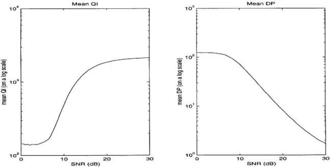
rela-tionship between the metrics and SNR. The most immediate observation is the monotonic relationship between the QI and the SNR levels. This relationship is illustrated in Figure 4-1. QI increases with increasing SNR; this suggests that a low QI implies a low SNR. DP exhibits similar behavior, with an inverse relationship to SNR, as expected. It is clear that the effects of noise do, indeed, reduce the demodulator's ability to extract the correct symbol timing phase and will directly impact the value of the metrics' as measures of the channel noise. The important question, however, is how high is the correlation between
channel noise and the metrics and which of the two metrics is more closely correlated to SNR. Once that is determined, it will remain to evaluate how that metric can be used to convey additional information about the channel noise.
Mean QI Mean DP 104 10, 10 -10 co-SNR(dB) SNR(dB)
Figure 4-1: Plot of Mean
QI
and Mean DP Values over SNR levels from OdB to 30dB Furthermore, it is pertinent to use the simulated data to verify the models developed in previous chapters. As detailed in Chapter 3, the expected phasejitter
can be modeled as having a Gaussian distribution for SNR levels greater than 10 dB. Section 3.3.2 derives the expected results for both theQI
and the DP using this approximation. Verifying that the simulated and the expected results match will confirm the model and the results.4.4.1 Deriving Distributions and Goodness-of-fit Testing
Once a relationship between the metrics and SNR has been established and their expected behavior has been verified, further characterization of the metrics is possible. The
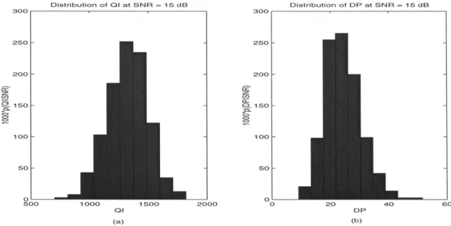
second-order statistics discussed in Section probability densities of the metrics function in Matlab, it is possible to to plot a bar graph representing the this binning is shown in Figure 4-2.
Distribution of 01 at SNR = 15 dB 300 1 20:0 5 s -00 1 1 so P 0 L 500 0
3.3.2 and Section 4.4 help to derive and verify the onditioned on a given SNR level. Using the hist bin the values of a vector of experimental data and distribution of the random variable. An example of Using this data, it is possible to test for particular
Distribution of DP at SNR = 15 dB 300! 250 200 1 so 100 so 2000 (a) 0 1 0 60 DP (b)
Figure 4-2: Sample Histograms of QI (a) and DP (b) samples at SNR = 15 dB
distributions.
Goodness-of-fit testing methods have been developed to provide a means to confirm the suspected distribution of a particular random variable. Both QI and DP can be treated as random variables with some unknown distribution. The Monte Carlo simulations provide us with observations of the the metrics at particular SNR levels. The means and the variances can be calculated empirically, and goodness-of-fit testing can be used to confirm
a distribution using these second-order statistics. [9] documents the method of testing followed in this study. Using the binning information derived from the hist function, it is possible use these methods to test for particular distributions.
Accurately characterizing the distributions of the metrics is crucial to continuing statisti-cal analysis on the data. Knowing the distribution of the metric, there are many well-defined methods of estimating SNR from a given QI or DP value that can be applied. For instance, if the distribution is unimodal, then we can use maximum likelihood estimation techniques to formulate a mapping between SNR levels and particular metric values.
4.4.2
Discriminating Between SNR Levels
Finally, a measure of a metrics' ability to successfully discriminate between two different SNR levels is difficult to capture. From the sections above, we know that we can calculate the mean and standard deviation of each metric as a function of SNR. For a given SNR level, we can define the expected range of that metric to be its mean plus or minus one standard deviation. This should represent the range in which the majority of the probability density falls; that is, it represents the most likely values the metric will take on given that the channel conditions are as defined by the particular SNR level.
In this way, two SNR levels are "distinguishable" if their expected ranges do not over-lap. The distance between distinguishable SNR levels will vary for each metric. Clearly, one metric is better than the other if it distinguishes between two SNR levels that are indistinguishable by the other.
Evaluating the metrics in this manner makes some statement on its ability to perform diversity selection. If the expected ranges are too large, the ability to discriminate between nearby SNR levels is hampered. Likewise, if the means at different SNR levels are too similar, this may also inhibit the metrics' ability to distinguish between levels. Therefore, a metric with distinct means for each SNR level and small variances will exhibit a greater ability to perform diversity selection.
Chapter 5
Results
Following the methods described in Chapter 4, a set of random QI and DP data was estab-lished at 61 different SNR levels (for SNR=0 dB to SNR=30 dB with 0.5 dB increments). Statistical analysis was performed on the data, and the results are presented in this chapter. This presentation will include a characterization of the data, where the possible probability distribution of the metrics are discussed. If a suitable distribution can be verified, the met-ric will undergo further analysis according to the experiments detailed in Section 4.4. For instance, it will be shown how the data can be used to derive information about the SNR level given certain assumptions. Finally, a treatment of the expected performance of these metrics will be offered. The following chapter will discuss some conclusions based on these results and propose several suggestions and possibilities for further or future work in this area.
5.1
Q1
The simplest way to begin a classification of the distribution of QI is to calculate the em-pirical means and standard deviations of the metric at particular SNR levels. This is easily done in Matlab using the test vectors generated by the Monte Carlo hardware simulations described in Chapter 4. Plots of the calculated means and the calculated variances of QI against a log scale of the dB levels at which they were measured is shown in Figure 5-1. Several things are observable from these plots. One is the monotonic relationship between the expected QI and the SNR level in the channel. It is clear that the effects of noise do, in-deed, affect QI values in a distinct relationship, and does thereby, reduce the demodulator's
Mean Q1 10" 10, Variance of 01 33 1o S d CN C) CO toS 3d 110 0102300 10 20 30 SNR (dB) SNR (dB)
Figure 5-1: Plot of Mean Q1 Values and its Standard Deviation over SNR levels from 0dB to 30dB
ability to extract the correct symbol timing phase. It is also notable that the QI begins to saturate after a certain SNR level, leading to the belief that a certain amount of degradation
occurs from ISI, and not inherently from other sources of noise. These are not effects that were considered as significant in the channel model, and therefore are not included in the analysis. However, they clearly have a role in affecting QI. These effects may reduce the power of the proposed methods in this study, and that degradation in performance will be
addressed in the conclusion.
From these plots, it is hoped that QI can be shown to have a direct relationship to SNR, whereby a QI value can give reliable information on the SNR level present on the channel. Note that what is shown in the plots in Figure 5-1 are QI values given a particular SNR level. These correspond to the distribution calculated in Chapter 3. Figure 5-2 demonstrates that the compiled data matches the expected results calculated in Section 3.3.2. Although the curves are not exact matches, they do, indeed, approximate each other. From this, the results derived in Chapter 3 can be considered valid approximations for the range of SNR levels specified.