Transport of aerosol to the Arctic: analysis of CALIOP and French aircraft data during the spring 2008 POLARCAT campaign

(1)

HAL Id: hal-01119972

https://hal.uca.fr/hal-01119972

Submitted on 24 Feb 2015

HAL is a multi-disciplinary open access

archive for the deposit and dissemination of

sci-entific research documents, whether they are

pub-lished or not. The documents may come from

teaching and research institutions in France or

abroad, or from public or private research centers.

L’archive ouverte pluridisciplinaire HAL, est

destinée au dépôt et à la diffusion de documents

scientifiques de niveau recherche, publiés ou non,

émanant des établissements d’enseignement et de

recherche français ou étrangers, des laboratoires

publics ou privés.

and French aircraft data during the spring 2008

POLARCAT campaign

Gérard Ancellet, Jacques Pelon, Yann Blanchard, Boris Quennehen, Ariane

Bazureau, Kathy S. Law, Alfons Schwarzenboeck

To cite this version:

Gérard Ancellet, Jacques Pelon, Yann Blanchard, Boris Quennehen, Ariane Bazureau, et al..

Trans-port of aerosol to the Arctic: analysis of CALIOP and French aircraft data during the spring 2008

POLARCAT campaign. Atmospheric Chemistry and Physics, European Geosciences Union, 2014, 14,

pp.8235-8254. �10.5194/acp-14-8235-2014�. �hal-01119972�

(2)

Atmos. Chem. Phys., 14, 8235–8254, 2014 www.atmos-chem-phys.net/14/8235/2014/ doi:10.5194/acp-14-8235-2014

Transport of aerosol to the Arctic: analysis of CALIOP and French

aircraft data during the spring 2008 POLARCAT campaign

G. Ancellet1, J. Pelon1, Y. Blanchard1, B. Quennehen2,1, A. Bazureau1, K. S. Law1, and A. Schwarzenboeck2 1_{Sorbonne Université, UPMC, Paris 06, Université Versailles St-Quentin, CNRS/INSU, LATMOS, Paris, France} 2_{Université B. Pascal, INSU/CNRS, Laboratoire de Météorologie Physique, Aubière, France}

Correspondence to: G. Ancellet (gerard.ancellet@upmc.fr)

Received: 13 December 2013 – Published in Atmos. Chem. Phys. Discuss.: 4 March 2014 Revised: 13 June 2014 – Accepted: 4 July 2014 – Published: 18 August 2014

Abstract. Lidar and in situ observations performed during the Polar Study using Aircraft, Remote Sensing, Surface Measurements and Models, Climate, Chemistry, Aerosols and Transport (POLARCAT) campaign are reported here in terms of statistics to characterize aerosol properties over northern Europe using daily airborne measurements con-ducted between Svalbard and Scandinavia from 30 March to 11 April 2008. It is shown that during this period a rather large number of aerosol layers was observed in the tropo-sphere, with a backscatter ratio at 532 nm of 1.2 (1.5 below 2 km, 1.2 between 5 and 7 km and a minimum in between). Their sources were identified using multispectral backscatter and depolarization airborne lidar measurements after care-ful calibration analysis. Transport analysis and comparisons between in situ and airborne lidar observations are also provided to assess the quality of this identification. Com-parison with level 1 backscatter observations of the space-borne Cloud-Aerosol Lidar with Orthogonal Polarization (CALIOP) were carried out to adjust CALIOP multispectral observations to airborne observations on a statistical basis. Recalibration for CALIOP daytime 1064 nm signals leads to a decrease of their values by about 30 %, possibly related to the use of the version 3.0 calibration procedure. No recalibra-tion is made at 532 nm even though 532 nm scattering ratios appear to be biased low (−8 %) because there are also signif-icant differences in air mass sampling between airborne and CALIOP observations. Recalibration of the 1064 nm signal or correction of −5 % negative bias in the 532 nm signal both could improve the CALIOP aerosol colour ratio expected for this campaign. The first hypothesis was retained in this work. Regional analyses in the European Arctic performed as a test emphasize the potential of the CALIOP spaceborne lidar for

further monitoring in-depth properties of the aerosol layers over Arctic using infrared and depolarization observations. The CALIOP April 2008 global distribution of the aerosol backscatter reveal two regions with large backscatter below 2 km: the northern Atlantic between Greenland and Norway, and northern Siberia. The aerosol colour ratio increases be-tween the source regions and the observations at latitudes above 70◦N are consistent with a growth of the aerosol size once transported to the Arctic. The distribution of the aerosol optical properties in the mid-troposphere supports the known main transport pathways between the mid-latitudes and the Arctic.

1 Introduction

It is recognized that long-range transport of anthropogenic and biomass burning emissions from lower latitudes is the primary source of aerosol in the Arctic (Quinn et al., 2008; Warneke et al., 2010). Frequent haze and cloud layers in the winter–spring period contribute to surface heating by their infrared emission (Garrett and Zhao, 2006). The relative influence of the different mid-latitude aerosol sources was initially discussed by Rahn (1981) who concluded that the Eurasian transport pathway is important using meteorolog-ical considerations and observations. Law and Stohl (2007) also stressed the seasonal change of air pollution transport into the Arctic with a faster winter circulation, implying a stronger influence of the southerly sources in the mid- and upper troposphere.

During the International Polar Year in 2008, these ques-tions were addressed in the frame of the Polar Study using

(3)

Aircraft, Remote Sensing, Surface Measurements and Mod-els, Climate, Chemistry, Aerosols and Transport (POLAR-CAT) and the Arctic Research of the Composition of the Tro-posphere from Aircraft and Satellites (ARCTAS) field exper-iments. Aircraft observations were conducted in spring 2008 over the European Arctic as part of POLARCAT-France (de Villiers et al., 2010; Quennehen et al., 2012) and over the North American Arctic, also called western Arctic in this paper, as part of ARCTAS (Jacob et al., 2010). Several pa-pers have already been published on the characterization of aerosols over the western Arctic (Brock et al., 2011; Rogers et al., 2011; Shinozuka et al., 2011). Overall, they provide a very useful data base to discuss the aerosol transport path-ways and the main processes driving their evolution when transported to the Arctic. Besides field experiments involving aircraft measurements, no systematic information was pro-vided until recently on regional Arctic aerosols by space ob-servations. The Cloud-Aerosol Lidar and Infrared Pathfinder Satellite Observation (CALIPSO) mission (Winker et al., 2009) has proven to be very useful for addressing these questions as illustrated by the recent work of Winker et al. (2013) although all its potential has not been explored yet. Recent studies using the Cloud-Aerosol Lidar with Orthogo-nal Polarization (CALIOP) level 2 products, namely the 5 km aerosol layer products (AL2) at 532 nm gridded for the Arctic domain, allowed aerosol extinction and aerosol optical depth (AOD) to be derived (Di Pierro et al., 2013). The main fea-tures of transport in the Arctic were inferred from the sea-sonal variability of the vertical distribution of aerosol, de-rived from AL2 version 3.0 products by Devasthale et al. (2011). Observations by the CALIOP lidar provide the op-tical properties of aerosol layers at two different wavelengths (532 nm, 1064 nm), but the infrared (IR) data have not been widely used due in large part to difficulties in the calibration of the level 1 (L1) products (Wu et al., 2011; Vaughan et al., 2012). In our study we thus address this topic looking for the usefulness of the additional information provided by the 1064 nm channel and depolarization measurements.

In this work, we focus on the European Arctic sector in spring 2008 using the data of the POLARCAT-France ex-periment. The purpose of this paper is thus to discuss how CALIOP spaceborne lidar data can be compared to and com-bined with aircraft data for the western Arctic area to pro-vide (i) a comparison of CALIOP observations with those from airborne lidar at similar wavelengths in a region where CALIOP data are very useful but not very well characterized, (ii) tracks for bias correction and use of L1 CALIOP observa-tions at 1064 nm and in the depolarization channel to analyse behaviour of colour and depolarization ratios, respectively, and (iii) an improved description of the spatial variability of aerosol sources and transport to the Arctic, and implications for a regional and monthly mean characterization.

We begin Sect. 2 with a description of the aircraft cam-paign lidar data and the meteorological context which also includes a characterization of the particles from in situ

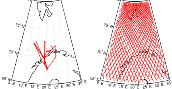
mea-Figure 1. Aircraft trajectories for the measurement days listed in

Table 1 (left) and positions of the CALIOP tracks from 27 March to 11 April (right).

surements and air mass transport using FLEXPART (FLEX-ible PARTicle dispersion model). The POLARCAT-France campaign was only described for some specific flights in previous papers (de Villiers et al., 2010; Quennehen et al., 2012). In Sect. 3, comparison between airborne and space-borne data are addressed, looking to the statistical distribu-tion and the spatial variability derived from all the aircraft flights available during POLARCAT-France, and coordinated CALIOP observations. In section 4, results obtained with monthly averaged L1 CALIOP data in April 2008 are used to analyse (i) the link between the meridional variability of the aerosol properties in relation to the air mass origin and (ii) the large scale horizontal variability in these aerosol properties for the whole Arctic domain. The latter is finally discussed with respect to the results obtained by previous analysis in-volving CALIOP AL2 products.

2 The POLARCAT spring campaign 2.1 Campaign context and description

The French ATR-42 was equipped with remote sensing in-struments (lidar, radar), in situ measuring probes of gases (O3, CO), and aerosols (concentration, size distribution). The ATR-42 deployment was often designed to collect data near CALIOP satellite observations during daytime overpasses. The positions of the 12 scientific flights performed from 30 March to 11 April 2008 (Fig. 1) show that they are well suited for an analysis of the meridional distribution near 20◦_{E. The}

meteorological context in the Arctic in April 2008 is dis-cussed in Fuelberg et al. (2010). The maps of the 700 hPa equivalent potential temperature (θe) and winds are, how-ever, shown in Figs. S1 and S2 of the Supplement to iden-tify the variability of the position of the Arctic front. This front was near 71◦N until 2 April and moved to lower lat-itudes near 68◦N after 2 April. It was observed that flights were frequently performed in the air masses strongly influ-enced by the southerly flow from Europe at the beginning of

(4)

G. Ancellet et al.: Transport of aerosol to the Arctic: analysis of CALIOP and aircraft data 8237 the campaign, while large section of the flights were

repre-sentative of the Arctic pristine air at the end of the campaign. After 9 April, the European Arctic at latitude above 70◦_N

became strongly influenced by advection of biomass burning plumes advected from Asia (Quennehen et al., 2012).

The vertical structure of the aircraft flight plans were al-ways chosen to have several in situ and airborne lidar mea-surements in similar air masses in order to study the represen-tativeness of lidar products such as the attenuated backscat-ter, the colour ratio and the depolarization ratio.

During the aircraft campaign, the CALIOP spaceborne in-strument provided 80 satellite overpasses for the period 27 March to 11 April in the area: 65–80◦N, 5–35◦E (Fig. 1). For the area south of 72.5◦N which corresponds to the aircraft deployment, there are 45 CALIOP tracks leading to 433 ver-tical profiles with 80 km horizontal resolution. In this work different temporal or spatial averaging will be used to analyse the CALIOP data either in the aircraft domain for compari-son with the airborne data (Sect. 3) or for the whole European Arctic area for all days in April 2008 (Sect. 4).

2.2 Aircraft data

2.2.1 Airborne lidar measurements

During the POLARCAT campaign, the airborne lidar Le-andre Nouvelle Generation, provided measurements in its backscatter configuration (hereafter simplified as B-LNG) of total attenuated backscatter vertical profiles at three wavelengths: 355, 532 and 1064 nm. An additional chan-nel recorded the perpendicular attenuated backscatter vertical profile at 355 nm. The B-LNG lidar is already described in de Villiers et al. (2010) (ADV2010) where a single flight on 11 April 2008 was analysed. The methodology to calibrate the attenuated backscatter is also fully described in ADV2010 so it is only briefly described here.

In this paper, aerosol layers are identified for the 12 flights using 20 s averages of lidar profiles (i.e. a 1.5 to 2 km hor-izontal resolution). Only downward-pointing lidar observa-tions have been included in this work. The B-LNG data are first corrected for energy variations. Calibration factors are then determined for each wavelength and for each flight by searching for areas with very low aerosol content and by as-suming that the Rayleigh contribution controls the lidar sig-nal. These areas are chosen, as far as possible, in the up-per altitude range close to the aircraft where bias due to the aerosol transmission does not play a significant role. The consistency of the calibration factor is checked using differ-ent aerosol free areas and several flights, whenever possible. This is the major source of error in the calculation of R(z), and the uncertainty (error and bias, but mostly due to bias) was found to be less than 15 % at 532 nm and less than 30 % at 1064 nm. These numbers were derived from a sensitivity study using different possible calibration factors and differ-ent flights. The two 355 nm channels are calibrated

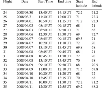
indepen-Table 1. Time and positions of the B-LNG lidar vertical cross

sec-tions during the POLARCAT spring campaign.

Flight Date Start Time End time Start End latitude latitude 24 2008/03/30 13:40 UT 14:15 UT 72.2 71.2 25 2008/03/31 11:30 UT 12:00 UT 71 72.3 26 2008/04/01 10:50 UT 11:15 UT 71.2 72.3 27 2008/04/03 08:15 UT 09:15 UT 68 71 27 2008/04/03 08:50 UT 09:50 UT 71 68 28 2008/04/06 12:30 UT 13:30 UT 69 72.7 29 2008/04/07 08:45 UT 09:15 UT 69.5 71 29 2008/04/07 10:20 UT 11:10 UT 72 70 30 2008/04/07 13:10 UT 13:45 UT 69.8 68 31 2008/04/08 08:45 UT 09:45 UT 68 71 31 2008/04/08 10:45 UT 11:30 UT 72 70 32 2008/04/08 13:10 UT 13:45 UT 70 68 33 2008/04/09 09:10 UT 09:50 UT 68 70.5 33 2008/04/09 11:00 UT 12:10 UT 71.5 67.8 34 2008/04/10 10:20 UT 11:20 UT 68 72 34 2008/04/10 12:45 UT 13:15 UT 70 68 35 2008/04/11 10:00 UT 11:30 UT 72.2 71.2 35 2008/04/11 12:30 UT 12:55 UT 69.2 68.2

dently using molecular reference and the ratio of the total perpendicular- to the total parallel-polarized signals. How-ever, due to a reduced field of view at 355 nm, the overlap of the emitted beam with the receiver field of view limits our ability to calibrate independently the total 355 nm lidar sig-nal in the areas near the aircraft selected at the other wave-lengths. Therefore, and as CALIOP is operating at 532 nm, the measurements at 355 nm are only used for the depolar-ization ratio analysis, which is less dependent on the geo-metrical factor. The B-LNG 355 nm ratio is only a proxy for the CALIOP one, as some differences are expected to occur due to wavelength difference (Freudenthaler et al., 2009).

The aerosol parameters discussed in this paper and the way to calculate them are fully described in ADV2010. They are the same for airborne and spaceborne observa-tions (although depending on the wavelength for depolar-ization). They are namely (i) the attenuated backscatter ra-tios R(z) at 532 nm and 1064 nm using the CALIOP atmo-spheric density model to calculate the Rayleigh backscat-ter vertical profiles, (ii) the ratio of the total perpendicular to the total parallel plus perpendicular polarized backscat-ter coefficient (or pseudo-depolarization ratio (PDR) δ355) at the measurement wavelength, 355 or 532 nm, respectively, (iii) the pseudo-colour ratio defined as the ratio of the to-tal backscatter coefficients at 1064 and 532 nm (PCR(z) =

R1064(z)/[16R532(z)] and (iv) the colour ratio defined as the ratio of the aerosol backscatter coefficients at 1064 and 532 nm (CRa(z) = (R1064(z) −1)/[16(R532(z) −1)]). The aerosol colour ratio can be also written as CRa(z) =2−k, where k is an exponent depending on the aerosol microphys-ical properties (Cattrall et al., 2005).

(5)

Figure 2. Distribution and cumulative probability (blue) of the 532 nm (top left) and 1064 nm (top right) backscatter ratios measured by the

B-LNG lidar from 30 March to 11 April. Mean, standard deviation, median and 90th percentile are given for each distribution. The distribution of the aerosol colour ratio CRa×16 (bottom) is compared to the lines for CRa=0.125 (k = 3), CRa=0.25 (k = 2) and CRa=0.5 (k = 1).

The vertical and latitudinal aircraft cross sections are listed in Table 1 and the corresponding R532 sections are shown in Fig. S3 of the Supplement. Clouds are removed from the lidar signals using a threshold both in scattering ratio and depolarization.

This data set composed of 18 lidar meridional cross sec-tions is a representative sample of the European Arctic spring aerosol distribution, as it includes different kinds of aerosol load in the lower troposphere and several cases of aerosol layers detected in the troposphere above 2 km. The probabil-ity densprobabil-ity function (PDF) of the retrieved R(z) are shown in Fig. 2 to check that the lidar data processing does not produce outliers for some flights. The homogeneity of the results be-tween the different flights has also been verified by dividing the lidar data into three subsets: one corresponding to the be-ginning of the campaign (before 7 April), the second one to the end (after 7 April) and the third to the overall campaign (see Table 1). The differences between the three subsets are small when looking at the means and standard deviations of the distributions meaning that the error related to the cali-bration procedure is independent of the selected flight (not shown). In Fig. 2, the R532(z)values do not exceed 2 (90th percentile = 1.45) with a mean value of 1.2, as expected for the Arctic troposphere where there are a lot of air masses with low aerosol load (Rodríguez et al., 2012). Both the IR and the green distribution show a high left tail in the his-togram. Although most of the aerosol scattering ratios are found near the median values (R532=1.15 and R1064=1.9),

the high left tail shows that air masses with R532>1.4 and

R1064>2.8 are also frequently found (probability > 75 %). The uncertainty of the mean values R532 and R1064 can be evaluated assuming 100 independent samples for the 18 cross sections shown in Fig. S3 of the Supplement, (i.e. three vertical layers and two horizontal layers) and errors of 0.1 and 0.5 for R532 and R1064, respectively, in a single layer. The distribution of the aerosol colour ratio shows a mean CRanear 0.31 ± 0.12, corresponding to a rather large wave-length dependence and thus to small particle size (k = 2). A small mode is seen to occur near 0.5 corresponding to much smaller wavelength dependence (k = 1) and thus to larger particles. We also obtain a value of 0.33 ± 0.04 for the colour ratio CR∗

a=

R1064−1

16(R532−1) calculated using the mean values of

R(z)(Fig. 2). Larger values near 0.5 are explained by the fact that at least 20 % of the 532 nm observations with moderate

R532values near 1.2 contribute to the tail of the R1064 distri-bution with values more than 2.4. The CRa values from the B-LNG are smaller than the range 0.4–1 (dust excepted) de-rived from the Aerosol Robotic Network (AERONET) using sun photometers at 26 sites across the globe (Cattrall et al., 2005). However, similar values have been reported for polar air masses using lidar measurements in Alaska and Canada (Burton et al., 2012) and for a smoke layer over Ny-Alesund (Stock et al., 2011).

Since the backscatter ratio distributions points toward a significant contribution of aerosol particles with small sizes

(6)

G. Ancellet et al.: Transport of aerosol to the Arctic: analysis of CALIOP and aircraft data 8239

Figure 3. Left – comparison of B-LNG lidar attenuated backscatter averaged 120 to 200 m below the aircraft in 2.5 × 10−5km−1sr−1with in situ measurements of CO (red) in ppbv and condensation particle counter (CPC) aerosol concentration (black) in cm−3for the flight 35. The green curve is the aircraft altitude in 5 m unit. Right – B-LNG lidar colour ratios (PCR and CRa) in % for 10 aerosol layers where in situ

and lidar data can be compared (see Table 2) versus the scanning mobility particle sizer (SMPS) aerosol mean diameter.

Table 2. Comparison of mean aerosol layer pseudo-(PCR) and aerosol (CRa) colour ratio measured by the B-LNG lidar and in situ

measure-ments: CO mixing ratio, GRIMM integral and CPC concentrations and the mean aerosol diameter Dmeanfrom the SMPS+GRIMM spectrum.

Layers data in italic or bold are respectively for low or high value colour ratios.

Date Time (UT) lat., dg alt. CO PCR B-LNG CRaB-LNG CPC GRIMM Dmean

km ppbv cm−3 cm−3 µm 30/03/08 13:45 72.0◦N 2.2 166 17.5 ± 1.5 % 38 ± 6 % 500 300 0.22 07/04/08 09:05 70.3◦N 4.5 153 8.7 ± 2 % 39 ± 64 % 450 50 0.07 08/04/08 11:20 70.7◦N 5.0 140 14.5 ± 2.3 % 62 ± 44 % 330 25 0.13 08/04/08 13:12 69.9◦N 1.0 153 10.0 ± 1.5 % 19 ± 6 % 800 25 0.07 08/04/08 13:17 69.7◦N 4.5 200 14.7 ± 1.6 % 27 ± 6 % 800 70 0.16 08/04/08 13:50 68.4◦N 4.0 220 17.0 ± 1.5 % 28 ± 4 % 1000 150 0.18 09/04/08 11:30 69.9◦N 4.5 210 10.0 ± 1.8 % 26 ± 16 % 2500 74 0.07 07/04/08 10:15 69.0◦N 4.0 210 11.0 ± 1.4 % 19 ± 5 % 1000 50 0.12 07/04/08 10:35 69.6◦N 3.5 230 18.7 ± 1.5 % 31 ± 4 % 900 300 0.22 07/04/08 11:05 71.6◦N 3.5 200 17.0 ± 1.6 % 42 ± 6 % 700 250 0.18

(Fig. 2), we thus looked at in situ measurements where com-parisons are possible.

2.2.2 Comparison of airborne lidar with in situ measurements

Aerosol and carbon monoxide (CO) in situ measurements available on the ATR-42 aircraft are described in Quennehen et al. (2012) and ADV2010. For the aerosols, a condensation particle counter (CPC-3010) measured the number of submi-cronic particles, while the aerosol concentrations in different size bins were measured by a Passive Cavity Aerosol Spec-trometer Probe (PCASP SPP-200), a GRIMM (model 1.108), and a scanning mobility particle sizer (SMPS) with a lower time resolution (150 s). In this paper we have used the SMPS

and the GRIMM data to compute the aerosol mean geomet-rical diameter with the 150 s time resolution. Comparisons of the CPC concentrations with the integrated concentrations of the eight size bins of the GRIMM between 0.3 and 3 µm, provide estimates of the relative fractions of coarse aerosol.

For flights with frequent vertical motion of the aircraft, it is easy to verify the comparability of lidar and in situ data. Such a comparison involves looking at in situ measurements only during aircraft ascents or descents crossing aerosol layers that the lidar detects later or earlier, respectively. An exam-ple of a comparison of the lidar attenuated backscatter mea-sured 150 m below the aircraft with CO and the CPC con-centrations is shown in Fig. 3 for the last flight on 11 April 2008, where rather large aerosol scattering ratios were mea-sured (see Fig. S3 of the Supplement). No delay correction

(7)

is performed for this figure to compensate for aircraft speed and lidar measurement distance (this is not detectable at this scale), but a high correlation (0.55 with significance better than 99 %) is nevertheless observed between lidar backscat-ter ratio and aerosol particle concentration.

Ten independent aerosol layers seen at nearly the same time by the lidar and the other instruments on board can be used for a meaningful comparison of the lidar parameters (colour and depolarization ratios) with the aerosol concen-tration and size spectrum (Table 2). The CO mixing ratios are well correlated with the CPC data implying that combus-tion aerosols were often encountered with the largest concen-trations at the end of the campaign. Changes in the pseudo-colour ratio PCR measured by the airborne lidar correspond quite well to the variations in the aerosol mean diameter be-cause R532 variations are small enough for these 10 layers to ensure a weak dependency with the aerosol concentration (Fig. 3). The increase of CRafrom 0.2 to 0.35 is also in good agreement with the variation in the aerosol mean geometri-cal diameter if we exclude the cases with the largest error on CRa. The uncertainty in the colour ratios are calculated assuming a 30 and 15 % relative uncertainty for the IR and green scattering ratio, respectively. According to Table 2, the largest colour ratios also correspond to the largest integrated GRIMM concentrations which are high for layers with coarse aerosol. The PCR and CRavalues calculated by the airborne lidar can be then considered as valuable proxies for evaluat-ing the contribution of the coarse aerosol fraction, and to first order (not considering speciation and size) the lidar backscat-ter ratio is a good indicator of aerosol content.

2.3 Characterization of air mass transport

The origin of the air masses sampled during the aircraft campaign by the B-LNG lidar and by CALIOP was stud-ied using the FLEXPART model version 8.23 (Stohl et al., 2002) driven by 6-hourly European Centre for Medium-Range Weather Forecasts (ECMWF) analyses (T213L91) in-terleaved with operational forecasts every 3 h. At a given lo-cation, the model was run to perform domain filling calcu-lations in 13 boxes from 1 to 7.5 km altitude with a hori-zontal dimension of 1◦×1◦. The transport from the different regions are considered for two altitude ranges: < 3 km and between 3 and 7 km in order to distinguish the two major transport pathways to the Arctic: low-level flow over cold surfaces and upper level advection by an uplifting along the tilted isentropes (Fuelberg et al., 2010; Stohl et al., 2006). This was done along the 18 aircraft cross sections and the 80 CALIPSO tracks in the European Arctic domain shown in Fig. 1. For each box, 2000 particles were released over 60 min and the dispersion computed for 6 days backward in time. Longer simulations lead to larger uncertainties in the source attribution and are not considered in this work. We have introduced in the FLEXPART model the calculation of the fraction of particles originating below the 3 km

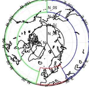
alti-Figure 4. Map of the regions selected to study the origin of the air

masses in the FLEXPART analysis. The red, green and blue boxes correspond to our definition of the European, North American and Eurasian regions. The two black boxes are called western and east-ern Arctic regions.

tude level for three areas with continental emissions shown in Fig. 4 (Europe, Eurasia, North America). We have also calcu-lated the fraction of particles present at latitudes above 70◦N in the troposphere above the eastern Arctic and western Arc-tic (black boxes in Fig. 4). The use of the eastern ArcArc-tic frac-tion is necessary to identify the role of the Eurasian sources because with our limited simulation time (6 days), we un-derestimate the role of aged air masses related to Eurasian emissions (ADV2010).

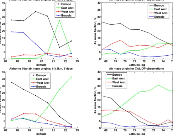
The results first show negligible influence of the transport from the lower troposphere above North America and are not considered further here. The fraction of air mass origins for the other regions is shown for different latitude bins in Fig. 5. The meridional distribution and the relative influence of the different regions are rather similar for the CALIPSO tracks and the airborne lidar flights in the lower atmosphere. However, in the mid-troposphere, the increase of the rela-tive influence of the eastern Arctic air versus European air masses is clearly shifted towards higher latitudes (74◦N) for CALIOP (no contribution in the 71–72◦N latitude band as seen for the airborne data). For both data sets, the transport of air masses from the eastern Arctic show a clear latitudi-nal increase in the lower altitude range just north of the po-lar front. For latitudes above 73◦N, seen only by CALIOP, the overall influence of all the selected source regions on a time scale shorter than 6 days remains, however, smaller than 40 %, implying that a large fraction of air masses had stayed for more than 6 days in the European Arctic sector located between −15◦W and 30◦E. Dilution, mixing and decay of the aged mid-latitude sources are to be expected

(8)

Figure 5. Latitudinal distribution of the fraction of observations corresponding to different air mass origins calculated with FLEXPART for

the airborne lidar (left column) and CALIOP observations (right column) at altitudes < 3 km (bottom row) and between 3 and 7 km (top row).

at these latitudes. The main differences between CALIOP and the airborne lidar sampling are (i) a significant contri-bution from Eurasian sources at low latitudes for the aircraft data and (ii) a weaker contribution of the eastern Arctic sec-tor in the mid-troposphere for CALIOP, especially around 70–72◦N. For the airborne lidar, the Eurasian sources were not only transported into the Arctic above the Pacific western coast but also by a low-level southerly flow over eastern Eu-rope from 6 to 9 April 2008. These differences are most prob-ably due to the much larger longitude band selected for the analysis of the CALIOP data set (5 to 35◦W) Despite these differences, the overall similarity of the transport regime for both data sets is a good indication that the small number of aircraft flights is fairly representative of the influence of the different source regions, and the data gathered may be used to compare retrieved aerosol properties in the campaign area.

3 Analysis of CALIOP data during the aircraft campaign

3.1 Methodology of the CALIOP data processing A detailed description of the CALIOP operational processing can be found in a series of papers (Vaughan et al., 2009; Liu et al., 2009; Omar et al., 2009; Powell et al., 2009).

Uncer-tainties in the AL2 colour ratio and the depolarization ratio are often very large and they are mainly used for a qualitative analysis of the aerosol composition and evolution (see Omar et al. (2009) for interpretation of the colour ratio and the de-polarization ratio for aerosol classification). Most of the er-ror in the colour ratio finds its origin in the signal calibration. More recently, analyses have been conducted to improve the calibration in version 4.0 (Vaughan et al., 2012), which con-firmed a bias in the 1064 nm channel and to a small extent the one in the 532 nm daytime channel. We thus considered a comparison between airborne and spaceborne CALIOP L1 observations as a first step.

In ADV2010, the AL2 CALIOP products were analysed for one particular flight of the POLARCAT campaign us-ing layers detected at 80 km horizontal resolution and with a 3 % threshold value for the layer optical depth at 532 nm. Comparisons between the CALIOP AL2 and airborne lidar PCR then showed larger values for CALIOP in the aerosol layers of the 11 April flight. Considering the large uncer-tainty in the weak aerosol layers detected in the AL2 product over the Arctic, averaging of the L1 version 3.01 CALIOP data is used in this paper to analyse the 45 CALIPSO tracks available in the aircraft campaign domain. The comparison of the aerosol parameter PDF obtained for the campaign pe-riod and the campaign area is considered as more appropriate

(9)

to validate the satellite aerosol data than relying on optimized collocations of aircraft and satellite data, which would give a very small number of cases. Gridded latitudinal distribu-tions with a 1.25◦resolution in the campaign area are used to check the coherency of the two data sets.

The CALIOP L1 attenuated backscatter coefficients β1064 and β532are available with 333 m horizontal resolution up to the 8.2 km vertical level and with 1 km resolution at higher altitude. Before making any horizontal or vertical averaging of these data, it is necessary to apply a cloud mask on the L1 data set. This cloud mask is based on the cloud mask features available in the level 2 version 3.01 CALIOP cloud (CL2) data products for the 5 km horizontal resolution. Additional checks have, however, been added to verify that cloud lay-ers are not misclassified. First, ice cloud laylay-ers, detected in the 80 km horizontal resolution profile, must have a pseudo-colour ratio > 0.6 and a layer depolarization ratio > 0.3. If this is not the case, the three brightness temperatures, T12 µm,

T10 µm and T8 µm, measured by the IR imaging radiometer (IIR) installed on the same platform (Garnier et al., 2012) are used as an additional test to classify the layer as a cloud layer or as an aerosol layer. Based on simulations, the crite-rion to keep a layer as a cloud layer is that the differences

T8 µm–T12 µm and T10 µm–T12 µmmust be positive (Dubuisson et al., 2008). Second, if the cloud layer is also detected in the 333 m resolution CL2 data products, it is always kept as a cloud as explained in Liu et al. (2009). Only very dense aerosol layers (scattering ratio > 3) are misclassified when adding these two conditions.

The β1064and β532data are then removed below the high-est cloud top altitude for each vertical profile, when the op-tical depth (OD) of the cloud is larger than 1. For semi-transparent clouds with smaller ODs (< 0.9), a transmission correction is performed. The data are also excluded in the 100 m layer just above the cloud top to avoid any error in the cloud top estimate. The cloud filtering is then very con-servative in order to exclude a possible bias in the aerosol parameters measured below clouds when the spectral varia-tion of the overlaying cloud attenuavaria-tion has to be taken into account.

The cloud-filtered 333 m attenuated backscatter vertical profiles are then over 80 km and vertically over 150 m with a low pass second-order polynomial filter second-order poly-nomial filter to improve the signal-to-noise ratio. The 80 km mean attenuated backscatter ratio R532(z)and R1064(z), the mean aerosol colour ratio and the mean 532 nm volume de-polarization ratio are finally calculated using the molecular density and ozone vertical profiles available at 33 standard altitudes in the CALIOP data products.

As explained before, two different methods are used for comparison with airborne lidar observations:

– PDF of aerosol parameters using all the 80 km, 150 m averaged profiles available in the aircraft campaign area, i.e. with 0 < z < 7 km, latitude between 65 and 72.5◦N,

longitude between 5 and 35◦_{E, from 27 March to 11}

April 2008

– a latitudinal cross section in the same campaign area where 80 km, 150 m averaged profiles are gridded into 5 × 14 boxes with a 1.25◦ latitude and 500 m vertical resolution.

3.2 Impact of the 1064 nm CALIOP calibration on the aerosol colour ratio

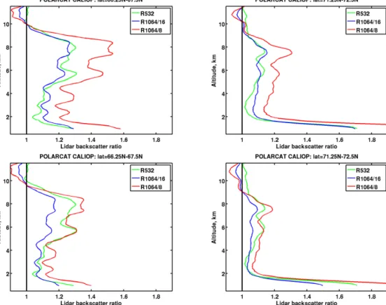
Two R532(z)mean profiles out of the 1.25◦gridded data set are compared with the corresponding R1064(z)mean profiles in Fig. 6. The R1064(z)is scaled to R532(z)to facilitate the comparison, assuming two extreme values of the expected aerosol colour ratio CRa(0.5 and 1), the range of values pro-posed by Cattrall et al. (2005). This corresponds to factors of 8 and 16, respectively, in the scaling of R1064(z) −1. For both latitude bins, a good consistency is obtained between the aerosol vertical structures at both wavelengths showing that the proposed averaging reduces the noise sufficiently to detect the mean aerosol layering at 1064 nm. The layer at 8 km can be used to identify the appropriate aerosol colour ratio because the spectral variation of the aerosol attenua-tion of the signal above the layer is not very important. With the lidar 1064 nm calibration factor used in the version 3.0 CALIOP L1 data products (see top figures in Fig. 6), the ra-tio between R532(z) −1 and R1064(z) −1 in this upper layer leads to CRanear 1 for both examples. This would mean that large dust-like aerosols contribute in both cases to the tro-pospheric aerosol in the European Arctic sector no matter which latitude band is chosen, which does not seem to be credible. Furthermore, depolarization remains low (< 5 %).

The 1064 calibration in the version 3.0 CALIOP data set is based on the assumption that for a specific set of cir-rus clouds, the cloud colour ratio is equal to 1 allowing the 532 nm calibration to be transferred to the 1064 channel. This is detailed in a large number of publications (Vaughan et al., 2010, 2012; Reagan et al., 2002; Winker et al., 2013). The cirrus cloud selection in version 3.0 implies an altitude range between 8 and 17 km and a minimum scattering ratio (> 50). The number of cirrus clouds with these characteristics is too small (< 11) for the campaign domain and period and no ad-ditional check was performed to verify the cirrus colour ratio. To reconcile the aerosol colour ratio with the expected value, three options are available: to decrease the 1064 to-tal backscatter, to increase the 532 nm toto-tal backscatter or to change both parameters. Considering the uncertainty of the 1064 nm channel (Vaughan et al., 2012) and the diffi-culty of estimating the respective impact of sampling dif-ferences and calibration error of the 532 nm CALIOP data (see Sect. 3.3), the 532 nm total backscatter values were not adjusted to the airborne data. The choice was to apply in-stead an a priori fixed multiplicative factor on the 1064 nm total backscatter, assuming a 40 and 30 % overestimate for

(10)

Figure 6. Mean attenuated backscatter ratio for the 532 nm (green) and 1064 nm filtered level 1 CALIOP (blue and red). The 1064 nm values

are scaled to the 532 nm values using expected lowest CRa=0.5 (red) and largest CRa=1 (blue). The top and bottom row respectively are

for uncorrected and calibration corrected IR data.

daytime and night-time conditions, respectively. For daytime this is estimated from the B-LNG mean scattering ratios (see Fig. 2). A reduced value was considered for night-time, as linked to the ratio in the daytime and night-time scale fac-tors in version 3.0 CALIOP data as mentioned in previous analyses (Wu et al., 2011; Vaughan et al., 2012). The ratio between R532(z)−1 and R1064(z)−1 then becomes more re-alistic since it leads to CRaintermediate between 0.5 and 1 for the upper layer near 8 km, and also for the layers in the lower troposphere.

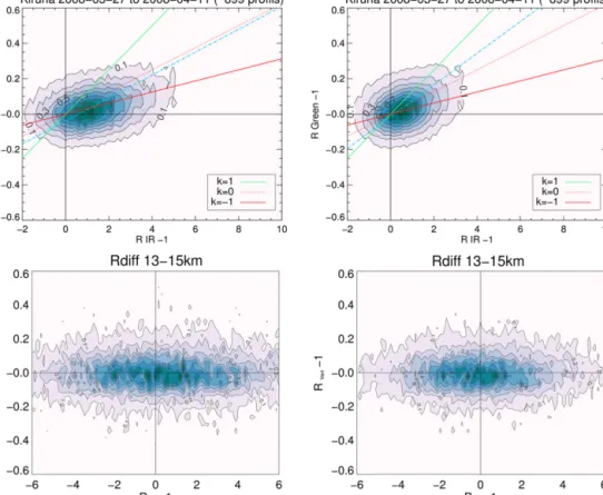
To verify that large CRafor uncorrected IR data is not re-lated to a bias introduced by the averaging of many profiles before the calculation of the colour ratio, we have looked at the R532(z)versus R1064(z)scatter plot using all the 80 km resolution CALIOP-filtered data for the altitude ranges, 0– 7 and 13–15 km. The scatter plots are presented in Fig. 7 for the uncorrected and corrected IR data using a frequency contour plot. Since we expect a very weak aerosol con-tribution in the 13–15 km altitude range, no specific cor-relation are found between R532(z) versus R1064(z). The noise of the 532 nm attenuated backscatter is of the order of 0.15 × molecular backscatter while the noise of the 1064 nm attenuated backscatter is 3 and 4 × molecular backscatter with and without the correction of IR data, respectively. Ac-counting for the factor of 16 between the two molecular

con-tributions, the noise in the IR channel is only 1.2 times larger than the 532 nm noise value when correcting the IR data. Such a ratio is comparable to the analysis of Wu et al. (2011) at 16 km for all the daytime CALIOP data. No correction of the IR would mean a ratio of 1.7 between the 532 and 1064 nm signal noise level. The overestimate of the 1064 nm backscatter is even more likely when looking at the scatter plot for the altitude range 0–7 km. The slope of the regression line is indeed too small for the uncorrected IR data since it corresponds to many CRavalues larger than 1. The frequency of clean air masses (R = 1) is also more consistent between the 532 nm and the 1064 nm observations after the correction of the IR overestimation provided that the 532 nm scattering ratio is correct.

The impact on the cirrus colour ratio was not evaluated for the small number of occurrences in our domain but it would imply a positive bias of 40 % when using the version 3.0 cal-ibration. Such a bias is larger that the uncertainty of ±20– 30 % proposed for the 1064 nm calibration procedure (Wu et al., 2011; Vaughan et al., 2012). We must recall, however, that a 40 % bias can be also accounted for if we assume a negative bias of 5 % for the 532 nm scattering ratio. As ex-plained in Sect. 3.3, this hypothesis was not considered in this work and the recalibration of the 1064 nm signal was chosen. It will be interesting to test this hypothesis using the

(11)

Figure 7. Correlation between the 532 and 1064 nm filtered level 1 CALIOP backscatter ratio from 27 March to 11 April 2008, at altitudes

from 0 to 7 km (top row) and 13 to 15 km (bottom row) using either uncorrected (left) or corrected (right) IR backscatter data. Regression line is the dashed-dotted blue line. The lines k = −1, 0, 1 are for tropospheric aerosol distributions with CRa=2, 1, 0.5m, respectively.

new version 4 level 1 CALIOP data which will be available. In the new version 4.0, the cirrus cloud selection for the 1064 calibration (i.e. with a cloud colour ratio of 1) has been up-dated (cloud temperature instead of altitude selection, use of the cloud depolarization ratio) providing more cirrus clouds and better altitude selection for the Arctic (Vaughan et al., 2012).

3.3 Comparison of airborne lidar and CALIOP 3.3.1 Analysis of the statistical distribution

Using the data set averaged over the campaign pe-riod/domain, the distributions of the CALIOP corrected

R1064and R532are shown in Fig. 8 for the range 0–7 km and 13–15 km. The latter corresponds to very low aerosol con-centrations. It has a mean and a median with a difference less than 0.02 at 532 nm and 0.3 at 1064 nm from the expected scattering ratio of 1. The large standard deviations of 0.3 at 532 nm and 4 at 1064 nm are expected at this altitude level where the molecular backscatter decreases significantly.

The R1064mean (2.3) is close to the airborne lidar value (2.1) considering an error of the mean of the order of 0.1 and even though the standard deviation of the noisy CALIOP

R1064distribution is 1.7 times larger than the airborne lidar corresponding value. The same ratio is observed between the airborne and CALIOP R532 standard deviation. Therefore, this confirms the validity of the estimated correction factor although with a large statistical error (about 30 % on the co-efficients) for the 1064 nm CALIOP profiles selected in our study of the Arctic region.

Contrary to the airborne lidar distribution, the CALIOP

R532 distribution in the troposphere below 7 km does not show many layers with elevated aerosol concentrations as shown by a lower value of the 90th percentile (1.34 for CALIOP instead of 1.45 for the airborne lidar). The larger standard deviation (0.34 instead of 0.2) is related to the poorer signal-to-noise ratio of the satellite data set. The lower value for the 532 nm mean (1.13 instead of 1.21) is larger than the expected uncertainty of the mean of the CALIOP distribution which is of the order of 0.01. This uncertainty of the mean is calculated assuming an error of 0.4 for a single CALIOP measurement (i.e. the width of the distribution for the negative values) and assuming 1700 independent layers out of 28 872 data points available in the 0 and 7 km altitude range above the campaign domain (i.e. considering a 1 km vertical sampling instead of the 60 m vertical resolution to ensure independence). Since we compare patchy data, it is

(12)

Figure 8. Distribution of the 532 nm (top left) and 1064 nm (top right) filtered level 1 CALIOP backscatter ratios at altitudes from 0 to 7 km

(green) and 13 to 15 km (red) from 27 March to 11 April in the aircraft flight area. Mean, standard deviation, median and 90th percentile are given for each distribution. The distribution of the aerosol colour ratio 16 × CRa(bottom) is compared to the lines for CRa=0.125 (k = 3),

CRa=0.25 (k = 2) and CRa=0.5 (k = 1).

also important to assess how the averaging of aerosol lay-ers with observed clear air scenes may explain this differ-ence. For example, the difference between the airborne and CALIOP R532 averages can be explained if there are twice as many layers with low aerosol load (R532<1.05) in the CALIOP data set. This may be related to the fact that in our CALIOP data processing we remove all the total backscatter values below clouds. It is also necessary to check whether this difference may also be due to (1) an overestimate of the 532 nm CALIOP calibration factor (2) an underestimate of the airborne lidar calibration factor. Positive differences due to 532 nm daytime calibration uncertainty were also obtained by Rogers et al. (2011) when comparing NASA High Spec-tral Resolution Lidar (HSRL) and CALIOP data for measure-ments at high latitudes in the Northern Hemisphere, but the mean difference is not higher than 3 %. The remaining 5 % uncertainty of the mean difference can be accounted for by a systematic error in the airborne lidar calibration when as-suming no aerosol in the altitude range which corresponds to the smallest attenuated backscatter coefficient. Comparisons with other observations confirmed that 532 nm CALIOP data could be underestimated by about 5 %, due to the occurrence of residual stratospheric aerosols at the normalization alti-tude (Vernier et al., 2009). This would be supported by the

fact that we obtain a very small value (< 2 %) of the 532 nm mean aerosol scattering ratio in the 13–15 km range when using the version 3.0 calibration.

The average CRa is 0.44 ± 0.8 for CALIOP which is not very far from the airborne lidar value (0.31 ± 0.12) consid-ering the factor of 6 between the two standard deviations of this parameter (Fig. 8). For the noisy satellite data, a better proxy is CRa

∗

=0.65 ± 0.1, i.e. the mean colour ratio calcu-lated with (R532−1) and (R1064−1), which is then 2 times larger than the similar ratio for the airborne lidar. This can be explained by the 10 % bias in R532 which is always less than 1.35. Therefore, this difference cannot be interpreted as a stronger contribution of the coarse aerosol fraction in the satellite observations. Despite this bias in the order of mag-nitude of CR∗

a, it is important to verify if the relative spatial or temporal variability is detected by the satellite data.

3.3.2 Analysis of the latitudinal distribution

The latitudinal variability of the aerosol properties is stud-ied using the CALIOP latitudinal grid data set described ear-lier, i.e. considering 5 successive 1.25◦latitude bins and 14 vertical layers of 500 m. The airborne lidar data are analysed only for layers where the aerosol content is high enough to be

(13)

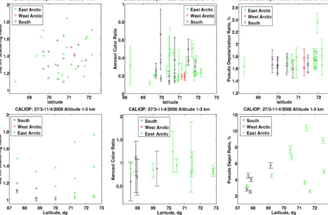
Figure 9. Latitudinal distribution of 532 nm backscatter ratio (left), aerosol colour ratio (middle) and pseudo-depolarization ratio (right) for

the airborne lidar observations (top) and filtered level 1 CALIOP (bottom) at altitudes < 3 km during the aircraft campaign. The colours are for different air mass origins estimated with FLEXPART (see text).

observed in the 1064 nm profiles. There are 90 well defined and independent aerosol layers identified in the 18 lidar cross sections at latitudes less than 72.5◦N. For the campaign pe-riod, we do not have many data below 1 km (see Fig. S3 in the Supplement), so the comparison of the latitudinal variations is made for the two following altitude ranges: 1–3 and 3– 7 km. The latitudinal distributions of R532, CRaand δ532(or

δ355) are shown for both data sets in Figs. 9 and 10. For each aerosol layer, the FLEXPART analysis was used to distin-guish between European or Eurasian air masses transported by the southerly flow on one hand, and the Eurasian or North American sources advected in our domain through the polar dome on the other hand. The green and red data points cor-respond to eastern and western Arctic origins, respectively, while the black points, labelled South in Figs. 9 and 10, in-dicate the influence of mid latitude sources directly advected by the southerly flow. Each point in the airborne lidar plots corresponds to a single layer observed by the aircraft, while for CALIOP it corresponds to an average of several layers at the same altitude in the selected latitude band.

Lower troposphere (< 3 km)

For the lower troposphere (Fig. 9), the airborne lidar does not show a clear latitudinal dependency of the aerosol scattering ratios for the eastern Arctic and European/Eurasian sources.

A decrease of the occurrence of elevated aerosol concentra-tions is, however, observed by CALIOP at the lowest lati-tudes. This is especially true for the eastern Arctic aerosol type. The increase of cloudiness at southern latitudes may ex-plain this evolution because of the lower probability of obser-vations in the lowermost troposphere. The significant number of CALIOP R532 values below 1.1 identified in the statisti-cal analysis discussed in the previous section is seen at all latitudes. Although the range of CRaare larger for CALIOP (0.6–1.1 instead of 0.2–0.5 for the airborne lidar), the relative latitudinal variations are somewhat similar with a maximum between 70 and 72◦N, especially when focusing on the east-ern Arctic air masses.

The δ355 values measured by the airborne lidar are less than 1.5 % for no depolarization and exceed 2 % when depo-larization is present, while the uncertainty is of the order of 0.2 %. Values of δ532measured by CALIOP are larger, rang-ing from 3 to 11 %, because of a spectral variation of the aerosol depolarization ratio. Assuming a backscatter ratio of the order of 1.1 at 355 nm and 1.3 at 532 nm, such a change of PDR corresponds to a change of the aerosol depolarization ratio from 5 % at 355 nm to 10 % at 532 nm. Such a spectral variation was observed by Gross et al. (2012) in a mixture of volcanic ash and marine aerosol when hygroscopic aerosol was present but at a size small enough to decrease only the 355 nm parallel backscatter. A similar kind of mixture could

(14)

the airborne lidar observations (top) and filtered level 1 CALIOP (bottom) at altitudes between 3 and 7 km during the aircraft campaign. The colours are for different air mass origins estimated with FLEXPART (see text).

exist in our European Arctic domain and was found in air-craft measurements over Alaska in April 2008 (Brock et al., 2011). Regarding the latitudinal increase of the depolariza-tion ratio, it was observed for both data sets.

Mid-troposphere (> 3 km)

For the mid-troposphere (Fig. 10), the latitudinal decrease of the backscatter ratio is observed in the airborne and the CALIOP lidar data, especially for the southerly flow. The CALIOP observations are never strongly related to the east-ern Arctic at latitudes less than 75◦N for altitudes above 3 km as discussed in Sect. 2.3. Thus, the comparison is only meaningful when considering the air masses advected by the southerly flow. For both data set, the latitudinal variations are consistent: a small increase of CRa, a decrease of the pseudo-depolarization ratio.

To conclude, there are significant differences in the mag-nitude of CRa (mainly related to differences in the magni-tude of R532) and in the magnitude of the depolarization ra-tio (related to the expected spectral variara-tion between 532 and 355 nm), but the spatial variations are rather similar for both data sets considering the limited coverage of the airborne data. The comparison of the R532 1.25◦ averaged vertical profiles is also useful to discuss the relative influ-ence of calibration error and sampling differinflu-ences between

CALIOP and the B-LNG airborne lidar (Fig. 11). For the al-titude ranges with the largest aerosol content (below 2 km and above 4 km), the order of magnitude of R532 is similar and varies in the same direction when increasing the latitude bin. The largest differences are in the 1.5 to 4 km altitude range corresponding to the lowest values of R532 where the CALIOP data are frequently below 1.1. Therefore, the bias in R532 is not only related to calibration issues, but also to the fact that the airborne lidar saw more air masses with sig-nificant aerosol content in the altitude range of 1.5 to 4 km. This may be related to the specific targeting of the aircraft flights to sample such layers and also to the fact that many of these layers are observed below 4 km in the frontal zone where overlying clouds (see Supplement) make the detection by the CALIOP overpasses more difficult. The wider longi-tude range chosen for the CALIOP data set do not compen-sate for this difference in the observed air masses. Since the difference in the magnitude of the 532 nm backscatter ratio is not only related to a calibration uncertainty in one instrument or both, but also to differences in the number of observations with low aerosol content in the altitude range 1.5 to 4 km, we choose not to apply any correction to the 532 nm CALIOP data set.

(15)

Figure 11. B-LNG lidar (left) and CALIOP (right) vertical profiles of the 532 nm backscatter averaged over a 1.25◦latitude band and for the aircraft period.

4 CALIOP characterization of the aerosol layer properties in April 2008

4.1 Latitudinal variability in the European Arctic In this section, the CALIOP data are now analysed for 30 days in April 2008 to improve further the signal-to-noise ra-tio. The latitudinal distribution of aerosol properties in the European Arctic is still derived using average CALIOP ver-tical profiles for 1.25◦latitude bins, but over a larger domain between 65 and 80◦N. Two specific altitude ranges (0–2 km and 5–7 km) have been selected because they correspond to the largest aerosol load identified in the mean vertical profile over the European Arctic (Fig. 11).

Lower troposphere (0–2 km)

In the lower troposphere, the meridional cross section of

R532 reveals that the largest aerosol scattering in the plan-etary boundary layer (PBL) is for air masses with an eastern Arctic origin and mainly in the Arctic frontal zone between 69 and 75◦N (Fig. 12). The large error bars correspond-ing to small aerosol loads encountered in the Arctic limit the quantitative analysis of the CRameridional distribution. The slight increase of CRawith latitude is mainly related to the variation of CRa with the air mass origin. The eastern Arctic aerosol layers show CRa>1 while air masses with a European origin correspond to CRa≈0.7. The δ532cross section shows significant depolarization (near 10 % for the monthly average) within the 70–73◦_{N latitude range.}

Con-sidering the high scattering ratios, the significant fraction of coarse aerosol (CRanear 1) and depolarization, a contribu-tion of ice crystal formacontribu-tion in the frontal zone is very likely in this latitude range. When excluding these specific cases, the European aerosol layers have larger depolarization than eastern Arctic air masses. Larger and more spherical aerosols for the eastern Arctic layers is not so surprising considering

aerosol ageing in air masses transported from Asia (Massling et al., 2007).

Mid-troposphere (5–7 km)

In the mid-troposphere (5–7 km), there is a general decrease in R532 with latitude for the European air masses, while it increases for air masses with an eastern Arctic origin. So in contrast to the PBL there is a minimum of aerosol contri-bution near 72◦N. This can be explained if one assumes a significant wet removal of particles during upward vertical transport within the Arctic front. As observed for the lower troposphere, CRavalues are lower for European air masses (near 0.5) than for Asian Arctic origin (near 0.8). We do not see the large depolarization values related to the possi-ble presence of ice crystals above 5 km, since they are not transported out of the PBL. However, the meridional distri-bution of the depolarization shows a clear decrease at the highest latitudes. The latitudinal increase of CRa associated with a decrease in depolarization could be explained by the increasing importance of aged anthropogenic aerosol and not to a strong influence of dust particles. The in situ analysis of the size distribution made in Quennehen et al. (2012) indeed showed that Asian anthropogenic aerosol contributed signif-icantly to the accumulation mode.

4.2 Large scale distribution in the Arctic domain April monthly averages for R532, CRa and δ532 have been calculated for the complete Arctic domain (latitude > 60◦_N)

in horizontal boxes of 300 km × 300 km. The CRavalues are only given when R532>1.25 to focus on the contribution of significant aerosol plumes, and to avoid large errors in CRa due to small scattering ratios. The fraction of CALIOP obser-vations available (i.e. not below a cloud) in the selected alti-tude range is also given to estimate the number of effective CALIOP tracks in every box. According to Fig. 1 a minimum

(16)

filtered level 1 CALIOP in April 2008 at altitudes < 2 km (bottom) and between 5 and 7 km (top). The origin of the layers are estimated with FLEXPART (see text).

number of 10 overpasses is needed for the data to be repre-sentative of a monthly mean. This corresponds to a fraction of 50 % at 65◦N and 20 % at 80◦N.

Lower troposphere (0–2 km)

In the lower troposphere (Fig. 13), the R532 map shows the extent of a northern Atlantic aerosol contribution with values remaining larger than 1.5 above 70◦N. Sea salt and sulfate aerosol are known to contribute to the increase of aerosol scattering over the North Atlantic in winter and early spring (Smirnov et al., 2000; Yoon et al., 2007). The CRamap indi-cates a gradual increase of CRawith latitude over the north-ern Atlantic: values < 0.7 occur near the mid-latitude sources located below 65◦N but CRa>0.9 are frequent above 70◦N. The latitudinal gradient of CRa over the northern Atlantic can be related to the growing influence of a different kind of aerosol, since the probability of aerosol particle trans-port from the eastern Arctic is increasing as discussed in the previous section. Aerosol composition analysis on board the NOAA ship during the International Chemistry Exper-iment in the Arctic Lower Troposphere (ICEALOT) cam-paign (Frossard et al., 2011) has shown that marine and sul-fate aerosol represent 70 % of the submicronic aerosol com-position in the northern Atlantic east of Iceland and they also

found that the sulfate contribution increases with latitude. This is broadly consistent with the CALIOP observations.

A local maximum in the R532map is also observed over Siberia between 90 and 110◦E with a latitudinal extent up to 70◦N in the Taymyr peninsula. In spring 2008, this area was known to have been influenced on one hand by local an-thropogenic emissions from gas flaring (Stohl et al., 2013), and on the other hand by early spring forest fires in Russia (Warneke et al., 2010). The maximum in northern Siberia is also seen for the same area in the AOD analysis made by Winker et al. (2013) using CALIOP data for the winter period before the fire period, implying a significant contribution of anthropogenic emissions. The CRavalues < 0.7 are similar to those observed below 65◦_{N over the Atlantic Ocean. No}

significant depolarization is observed in these two source re-gions implying very little impact from dust or volcano emis-sions in this altitude range. The difference of CRabetween the European Arctic and the source region in Russia implies a growing of the aerosol particles during transport and age-ing if one assumes that most of the aerosol layers observed in European Arctic originate from Eurasia (see previous sec-tion).

(17)

Figure 13. Map of the 532 nm backscatter ratio (top left), aerosol colour ratio (top right), pseudo-depolarization ratio (bottom left) and

fraction of cloudless observations (bottom right) using the April 2008 filtered level 1 CALIOP data in the 0–2 km altitude range. Colour scales are in relative units.

Mid-troposphere (5–7 km)

In the mid-troposphere (Fig. 14), the R532map gives a very different picture of the link between the Arctic aerosol dis-tribution and the mid-latitude sources. There is, first, a broad aerosol maximum from eastern Siberia to western Alaska at latitudes between 60 and 75◦_{N and, second, another}

maxi-mum over the Hudson bay. The eastern Arctic domain north of 70◦N is not as clean as in the lower troposphere, be-ing consistent with an efficient transport pathway from mid-latitudes along the tilted isentropic surfaces (Harrigan et al., 2011). The western Arctic and northern Atlantic are rela-tively free of aerosol particles in the mid-troposphere. This is somewhat contradictory with the known uplift of low-level North American air pollution over western Greenland (Har-rigan et al., 2011; Ravetta et al., 2007). The contrast between the large aerosol concentrations found in the northern At-lantic lower troposphere and the low values above is also consistent with the conclusions of several papers (Law and Stohl, 2007; Harrigan et al., 2011) about the transport path-way of European emission being most efficient in the lower troposphere.

The global cloud distribution can be obtained from the DARDAR (raDAR/liDAR) products, which are based on CloudSat and CALIOP data according to a variational scheme, on a 60 m vertical resolution and 1 km horizontal resolution grid (Delanoë and Hogan, 2008). The synergy be-tween lidar and radar is indeed needed to have a detailed pic-ture of the cloud vertical profile (Ceccaldi et al., 2013). It has

been used here to calculate the cloud fraction at different al-titudes during the month of April 2008 in 4 different latitude bands from 60 to 80◦_{N (Fig. 15). The latitudes with large}

cloudiness in both the mid and upper troposphere show up-ward frontal lifting by warm conveyor belts (WCB) near the Bering Strait and the western coast of Greenland. The lat-ter shows the largest cloudiness at 5 km. This may explain the low aerosol concentration downwind of Greenland due to efficient removal of aerosol. One can also notice the good correlation between the high values of the low-level cloud fraction and the large aerosol load observed above 70◦N in the European Arctic.

The aerosol depolarization and colour ratio distributions show little depolarization (except over the Hudson bay) in the large scale aerosol plumes seen in the mid-troposphere. However, as in the lower troposphere, the CRaincrease at lat-itudes > 70◦_{N is consistent with aerosol ageing when}

reach-ing the highest latitudes.

5 Conclusions

In this paper we have analysed aerosol airborne (B-LNG) and spaceborne (CALIOP) lidar data related to the transport of mid-latitude sources into the Arctic. The main results are the following:

– A campaign was held in April 2008 in the European Arctic with 18 aircraft cross sections and 80 CALIPSO tracks over 15 days improving our ability to identify the

(18)

Figure 14. Map of the 532 nm backscatter ratio (top left), aerosol colour ratio (top right), pseudo-depolarization ratio (bottom left) and

fraction of cloudless observations (bottom right) using the April 2008 filtered level 1 CALIOP data in the 5–7 km altitude range. Colour scales are in relative units.

Figure 15. Zonal vertical cross sections of the cloud fraction derived from the DARDAR products for April 2008 in 4 latitude bands from 60

to 80◦N. The longitudinal resolution is 5◦and the vertical resolution is 60 m.

transport of aerosol layers to the Arctic, especially from the analysis of the satellite data.

– Analysis of the B-LNG backscatter ratio R532and R1064 at two wavelengths for the calculation of the aerosol colour ratio (CRa) has been successfully compared with in situ aerosol measurements on board the aircraft. The CRa increase corresponds to a similar increase in

the mean aerosol diameter, showing the importance of multi-wavelength analysis. It also emphasizes the need for accurate lidar calibration.

– Simulations with the FLEXPART model show that the limited number of airborne lidar cross sections are rep-resentative of the main characteristics of the air mass transport in April 2008: increase with latitude of the

(19)

aged air masses from the eastern Arctic region at alti-tudes below 3 km, large influence of the mid-latialti-tudes sources directly transported by the southerly flow at al-titudes above 3 km.

– Comparisons are performed between B-LNG and CALIOP backscatter ratio R532and R1064at two wave-lengths, including the calculation of the aerosol colour ratio and of the depolarization ratio (PDR) at 532 and 355 nm. Comparisons are based on the analysis of 15-day averages and L1 CALIOP data processing instead of AL2 CALIOP operational products. Specific aver-aging methods can then be applied. The cloud screen-ing, needed when using L1 lidar data, is based on CL2 CALIOP data products and the IR CALIPSO ra-diometer data. A recalibration of the CALIOP R1064 in the Arctic was chosen to reduce the positive bias of the CALIOP data with respect to airborne observations of the colour ratio. A fixed factor was applied to the 1064 nm attenuated backscatter data, of 1.3 and 1.4, re-spectively, for night-time and daytime orbits. This value could be significantly smaller if a small negative bias of the 532 nm CALIOP lidar signal is also corrected, but this hypothesis was not applied in this work. The use of the new version 4.0 data which will be available very soon would certainly help to address this question.

– Comparisons of the statistical distributions in the alti-tude range 0–7 km show no significant bias for R1064 when correcting the CALIOP 1064 nm data but a −8 % difference between the CALIOP and B-LNG R532data. The latter might be related to a calibration problem of either the B-LNG or the CALIOP instrument. However, being largest in a specific altitude range between 1.5 and 4 km, the differences of the spatial averaging of airborne and satellite data are also to be considered. The differ-ence in the magnitude of CRais mainly related to this overestimation of R532 in the B-LNG data. The depo-larization ratio is not measured at the same wavelength and its spectral variation follows that of hygroscopic aerosol often at a size small enough to be detected only at 355 nm (Gross et al., 2012).

– The latitudinal distribution of the colour ratio and the depolarization ratio is similar for the B-LNG and the CALIOP data sets, especially considering the limited number of aircraft flights. It is a good indication that, despite possible bias in these two parameters when com-paring them, airborne and satellite data are still valuable for the analysis of the aerosol growth or the relative frac-tion of dust or volcanic ashes using CALIOP observa-tions.

– The monthly average analysis of the CALIOP colour and depolarization ratio in the European Arctic area shows that larger (higher CRa) and more spherical

aerosol (low PDR) are expected in the air masses trans-ported from the eastern Arctic both in the lower tropo-sphere (0–2 km) and in the mid-tropotropo-sphere (5–7 km). Less aerosol is present in the mid-troposphere near the arctic front (70–74◦N) while significant R532and depo-larization ratio are seen in the lower troposphere, possi-bly related to the presence of ice crystals.

– The global distribution of the CALIOP monthly anal-ysis reveal two regions with large backscatter below 2 km: the northern Atlantic between Greenland and Norway, and the Taymyr peninsula. The CRa increase between the source regions and the observations at lat-itudes above 70◦_{N implies a growth of the aerosol size}

once transported to the Arctic. The distribution of the aerosol optical properties in the mid-troposphere is con-sistent with the transport pathways proposed in Harri-gan et al. (2011): (i) low-level advection in northern Eu-rope, (ii) isentropic uplifting of pollution and biomass burning aerosol in northern Siberia and eastern Asia and (iii) aerosol washout by the North Atlantic warm con-veyor belts.

The Supplement related to this article is available online at doi:10.5194/acp-14-8235-2014-supplement.

Acknowledgements. The UMS SAFIRE is acknowledged for

supporting the ATR-42 aircraft deployment and for providing the aircraft meteorological data. The POLARCAT-France and CLIMSLIP projects were funded by ANR, CNES, CNRS/INSU and IPEV. The FLEXPART team (A. Stohl, P. Seibert, A. Frank, G. Wotawa, C. Forster, S. Eckhardt, J. Burkhart, H. Sodemann) is acknowledged for providing the FLEXPART code. NASA, CNES, the ICARE and the LARC data centre are gratefully acknowledge for supplying the CALIPSO data.

Edited by: G. Vaughan

References

Brock, C. A., Cozic, J., Bahreini, R., Froyd, K. D., Middlebrook, A. M., McComiskey, A., Brioude, J., Cooper, O. R., Stohl, A., Aikin, K. C., de Gouw, J. A., Fahey, D. W., Ferrare, R. A., Gao, R.-S., Gore, W., Holloway, J. S., Hübler, G., Jefferson, A., Lack, D. A., Lance, S., Moore, R. H., Murphy, D. M., Nenes, A., Novelli, P. C., Nowak, J. B., Ogren, J. A., Peischl, J., Pierce, R. B., Pilewskie, P., Quinn, P. K., Ryerson, T. B., Schmidt, K. S., Schwarz, J. P., Sodemann, H., Spackman, J. R., Stark, H., Thomson, D. S., Thornberry, T., Veres, P., Watts, L. A., Warneke, C., and Wollny, A. G.: Characteristics, sources, and transport of aerosols measured in spring 2008 during the aerosol, radiation, and cloud processes affecting Arctic Climate (ARCPAC) Project, Atmos. Chem. Phys., 11, 2423–2453, doi:10.5194/acp-11-2423-2011, 2011.