HAL Id: hal-03158975
https://hal.archives-ouvertes.fr/hal-03158975
Submitted on 4 Mar 2021
HAL is a multi-disciplinary open access
archive for the deposit and dissemination of
sci-entific research documents, whether they are
pub-lished or not. The documents may come from
teaching and research institutions in France or
abroad, or from public or private research centers.
L’archive ouverte pluridisciplinaire HAL, est
destinée au dépôt et à la diffusion de documents
scientifiques de niveau recherche, publiés ou non,
émanant des établissements d’enseignement et de
recherche français ou étrangers, des laboratoires
publics ou privés.
Spectroscopy and polarimetry of the gravitationally
lensed quasar SDSS J1004+4112 with the 6m SAO RAS
telescope
L. Č. Popović, V. Afanasiev, A. Moiseev, A. Smirnova, S. Simić, Dj. Savić, E.
Mediavilla, C. Fian
To cite this version:
L. Č. Popović, V. Afanasiev, A. Moiseev, A. Smirnova, S. Simić, et al.. Spectroscopy and polarimetry
of the gravitationally lensed quasar SDSS J1004+4112 with the 6m SAO RAS telescope. Astronomy
and Astrophysics - A&A, EDP Sciences, 2020, 634, pp.A27. �10.1051/0004-6361/201936088�.
�hal-03158975�
c
ESO 2020
Astrophysics
&
Spectroscopy and polarimetry of the gravitationally lensed quasar
SDSS J1004+4112 with the 6m SAO RAS telescope
?
L. ˇ
C. Popovi´c
1, V. L. Afanasiev
2, A. Moiseev
2,3, A. Smirnova
2, S. Simi´c
4, Dj. Savi´c
1,5,
E. G. Mediavilla
6,7, and C. Fian
61 Astronomical Observatory, Volgina 7, 11000 Belgrade, Serbia
e-mail: [email protected]
2 Special Astrophysical Observatory of the Russian AS, Nizhnij Arkhyz, Karachaevo-Cherkesia 369167, Russia 3 Space Research Institute, Russian Academy of Sciences, Profsoyuznaya ul. 84/32, Moscow 117997, Russia 4 Faculty of Sciences, University of Kragujevac, Radoja Domanovica 12, 34000 Kragujevac, Serbia
5 Université de Strasbourg, CNRS, Observatoire Astronomique de Strasbourg, UMR 7550, 11 rue de l’Université, 67000 Strasbourg,
France
6 Instituto de Astrofísica de Canarias, Viá Láctea s/n, La Laguna 38200, Tenerife, Spain 7 Departamento de Astrofísica, Universidad de la Laguna, La Laguna 38200, Tenerife, Spain
Received 13 June 2019/ Accepted 10 December 2019
ABSTRACT
Context.We present new spectroscopic and polarimetric observations of the gravitational lens SDSS J1004+4112 taken with the 6 m
telescope of the Special Astrophysical Observatory (Russia).
Aims.In order to explain the variability that is observed only in the blue wing of the C IV emission line, corresponding to image A, we analyze the spectroscopy and polarimetry of the four images of the lensed system.
Methods.Spectra of the four images were taken in 2007, 2008, and 2018, and polarization was measured in the period 2014–2017. Additionally, we modeled the microlensing effect in the polarized light, assuming that the source of polarization is the equatorial scattering in the inner part of the torus.
Results.We find that a blue enhancement in the C IV line wings affects component A in all three epochs. We also find that the UV
continuum of component D was amplified in the period 2007–2008, and that the red wings of CIII] and C IV appear brighter in D than in the other three components. We report significant changes in the polarization parameters of image D, which can be explained by microlensing. Our simulations of microlensing of an equatorial scattering region in the dusty torus can qualitatively explain the observed changes in the polarization degree and angle of image D. We do not detect significant variability in the polarization parameters of the other images (A, B, and C), although the averaged values of the polarization degree and angle are different for the different images.
Conclusions.Microlensing of a broad line region model including a compact outflowing component can qualitatively explain the C IV blue wing enhancement (and variation) in component A. However, to confirmed this hypothesis, we need additional spectroscopic observation in future.
Key words. gravitational lensing: strong – quasars: individual: SDSS J1004+4112 – line: profiles – polarization
1. Introduction
A lensed quasar is an active galactic nucleus (AGN) that is assumed to have a central supermassive black hole, surrounded by an accretion disk (which emits mostly in the X-ray from the inner part, but also in the UV/optical continuum in the outer disk part). The X/UV emitted radiation from the accretion disk pho-toionizes the surrounding matter, generating a region that is able to emit (in the process of recombination) broad emission lines, the so-called broad line region (BLR). Farther out, a torus-like dust region is thought to lie that mostly emits in the infrared (see, e.g.,Stalevski et al. 2012a;Netzer 2015).
The different regions of the AGN have emission peaks at different wavelengths, and they have different dimensions; microlensing magnification therefore affects them differently (see, e.g., Jovanovi´c et al. 2008). This can explain the varia-tions observed in the spectrum of a microlensed image (chro-matic microlensing, see, e.g.,Popovi´c & Chartas 2005).
? The reduced spectra are only available at the CDS via
anony-mous ftp to cdsarc.u-strasbg.fr(130.79.128.5) or viahttp: //cdsarc.u-strasbg.fr/viz-bin/cat/J/A+A/634/A27
Variations in the spectra of a lensed quasar image that are due to microlensing can be used to explore the innermost structure of lensed quasars (see, e.g.,Popovi´c et al. 2001a;Abajas et al. 2002;Popovi´c & Chartas 2005; Sluse et al. 2007;Blackburne et al. 2011;Fian et al. 2016,2018, etc.)
Spectroscopy has been used in several papers to constrain the sizes of different emission regions in lensed quasars, from γ-ray (see, e.g., Torres et al. 2003; Donnarumma et al. 2011;
Neronov et al. 2015; Vovk & Neronov 2016, etc.), X-ray (see e.g.Chartas et al. 2002;Popovi´c et al. 2001b,2003,2006;Dai et al. 2003,2004;Ota et al. 2006;Chartas et al. 2012,2017;Chen et al. 2013;Krawczynski & Chartas 2017, etc.), and UV/optical (see, e.g.,Popovi´c et al. 2001a;Abajas et al. 2002,2007;Popovi´c & Chartas 2005;Motta et al. 2012;Sluse et al. 2012;Braibant et al. 2017;Fian et al. 2018) to the infrared (see, e.g.,Stalevski et al. 2012b;MacLeod et al. 2013;Sluse et al. 2013;Vives-Arias et al. 2016).
One of the greatest interests is to constrain the inner-most structure of AGN (see, e.g.,Jiménez-Vicente et al. 2014;
Braibant et al. 2017;Hutsemékers et al. 2017) and especially the BLR (Popovi´c et al. 2001a;Abajas et al. 2002;Sluse et al. 2012;
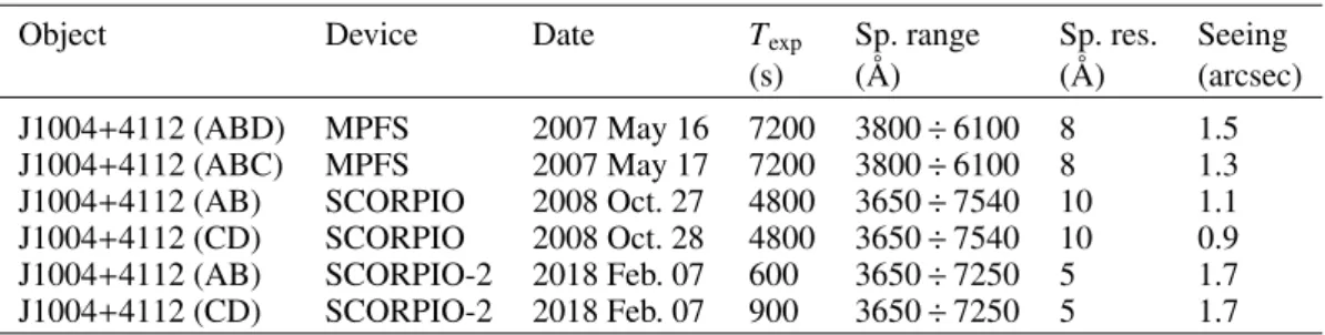
Table 1. Log of spectral observations of the lensed quasar J1004+4112 with the 6 m telescope.
Object Device Date Texp Sp. range Sp. res. Seeing
(s) (Å) (Å) (arcsec)
J1004+4112 (ABD) MPFS 2007 May 16 7200 3800 ÷ 6100 8 1.5
J1004+4112 (ABC) MPFS 2007 May 17 7200 3800 ÷ 6100 8 1.3
J1004+4112 (AB) SCORPIO 2008 Oct. 27 4800 3650 ÷ 7540 10 1.1
J1004+4112 (CD) SCORPIO 2008 Oct. 28 4800 3650 ÷ 7540 10 0.9
J1004+4112 (AB) SCORPIO-2 2018 Feb. 07 600 3650 ÷ 7250 5 1.7
J1004+4112 (CD) SCORPIO-2 2018 Feb. 07 900 3650 ÷ 7250 5 1.7
Guerras et al. 2013; Braibant et al. 2017; Hutsemékers et al. 2017), because this region is assumed to be relatively close to the central supermassive black hole, and consequently, the broad emission lines can be used to measure the masses of central black holes (seePeterson 2014;Mediavilla et al. 2018). However, to use the broad lines as a tool for black hole mass measurements, the kinematics and dimensions of the BLR have to be knonw. These can be studied from the impact of microlensing (see, e.g.,
Popovi´c et al. 2001a;Abajas et al. 2002;Braibant et al. 2017;
Hutsemékers et al. 2017;Fian et al. 2018, etc.).
Additionally, spectropolarimetric observations can give use-ful information about the quasar structure in general (see, e.g.,
Smith et al. 2004;Afanasiev et al. 2014,2019, etc.), especially in the case of lensed quasars (see, e.g.,Hutsemékers et al. 1998,
2015;Belle & Lewis 2000;Hales & Lewis 2007, etc.). The polar-ization in spectra of lensed quasars can give more information about the scattering region (assumed to be a torus) as well as about the kinematics of the BLR (see, e.g.,Hutsemékers et al. 2015). Unfortunately, the images of lensed quasars are faint sources, and in most cases, the images are very close such that they cannot be resolved and observed in spectropolarimetric mode. However, the broad band polarization of the total image is easier to carry out in order to study the changes in the polarization parameters (Stokes Q and U parameters) in a microlensing event.
Here we present new spectroscopic and polarimetric obser-vations of the lensed quasar SDSS J1004+4112, a four-image system with source redshift zs= 1.734 and lens redshift zl= 0.58
(Inada et al. 2003; Oguri et al. 2004). This system exhibits an unusually large separation between images of even 15.000 (for more details, seeInada et al. 2003;Oguri et al. 2004;Williams & Saha 2004). SDSS J1004+4112 is also interesting because of the
variability of the broad emission lines in component A. The vari-ability is observed in the blue wing of C IV and is not observed in the continuum or in the low-ionization lines (see, e.g.,Richards et al. 2004;Lamer et al. 2006;Green 2006;Gómez-Álvarez et al. 2006;Fian et al. 2018).
First,Richards et al.(2004) reported a 28-day-long ampli-fication event in the broad emission lines of component A that was observed in 2003. A second enhancement observed in 2004 was reported by Gómez-Álvarez et al. (2006) and confirmed byLamer et al. (2006). These events are difficult to explain in terms of gravitational microlensing because the expected follow-up amplification in another part of the line profiles has not been detected (as expected in the microlensing of a disk-line profile, e.g., see Popovi´c et al. 2001a). Additionally, there is no detec-tion of a continuum amplificadetec-tion that should be present dur-ing the BLR microlensdur-ing event because the BLR surrounds the compact continuum source. An alternative explanation of the J1004+4112 line variability was given by Green (2006), who assumed that the variability in the C IV blue wing of component A is caused by the absorption rate that is coming from matter
sur-rounding the QSO center. In this case, the difference between A and the other images could be due to the small viewing angle differences that result in slightly different light paths through the intervening matter. However, this explanation has been ruled out because the model predicts a significant X-ray absorption in components B, C, and D, which has not been observed (see
Lamer et al. 2006).
The question of the origin of the C IV A component variation in J1004+4112 remains unsolved, and it motivates us to con-tinue observing this lensed quasar. We obtained spectroscopic observations of J1004+4112 in three different epochs from 2007 to 2018 and polarimetric observations in the period 2014–2017 using the 6m telescope of the Special Astrophysical Observatory (SAO).
The paper is organized as follows: In Sect. 2 we describe our observations, and in Sect. 3 we explain the methodology. The results are shown in Sect.4, and the main conclusions are summarized in Sect.5.
2. Observations
2.1. MPFS observations and data reduction
J1004+4112 was observed with the integral-field MultiPupil Fiber Spectrograph (MPFS) located at the prime focus of the 6 m telescope of the SAO of the Russian Academy of Sciences (SAO RAS). MPFS takes simultaneous spectra from 256 spatial ele-ments (constructed in the shape of square lenses) that form an array of 16 × 16 elements on the sky with an angular size of 1 arcsec/element (seeAfanasiev et al. 2001). Behind each lens an optical fiber directs the light to the spectrograph slit. The sky back-ground spectrum was simultaneously taken with another fiber bundle placed at a distance of ∼4 arcmin from the lens array. The detector we used was an EEV42-40 (2K × 2K pixels) CCD. Addi-tional information about the observations is given in Table1.
The data reduction procedure has been described in sev-eral papers (see, e.g., Smirnova et al. 2007). Reduction yields a data cube with an individual spectrum in each pixel in the 16 × 16 arcsec field. Spectra from spectrophotometric standard stars were used to convert counts into absolute fluxes (Fλ). We observed the object twice because the angular distance between images C and D exceeds the MPFS field of view. During the first night, the MPFS array was centered to collect spectra of images A, B, and D, and during the second night, we observed images A, B, and C (see pointings of MPFS in Fig.1). After the primary data reduction, these two cubes were matched and combined into a mosaic cube with a resulting field of view of 18 × 24 arcsec2.
To reproduce spectra of each component, we collected the integrated spectra taking several bright pixels at the position of the image in apertures of 1.5–2 arcsec in radius. The Hubble Space Telescope (HST) image of this lensed system suggests a nearby object within 2 arcsec of component A (see Fig. 1 in
Fig. 1.Image from the 6 m telescope SCORPIO-2 (V-band, seeing ≈100
) of the field around J1004+4112: four components of the gravitational lens and three reference stars are labeled. Green lines represent the posi-tion of the spectrograph slits. Red and orange rectangles correspond to the two MPFS fields used during the observations.
Sharon et al. 2005). In our MPFS observations we were unable to correctly deblend this object. However, the possible contribu-tion of this galaxy in the integrated C IV emission line is lower than 5%, according the flux estimation in the MPFS data cube in the corresponding location.
2.2. Long-slit observations
The long-slit spectra of the four components of J1004+4112 were observed at the prime focus of the SAO RAS 6 m tele-scope in October 2008 and February 2018 with the multi-mode focal reducer SCORPIO (Afanasiev & Moiseev 2005) and its improved version SCORPIO-2 (Afanasiev & Moiseev 2011). A long-slit with a width of 1 arcsec was placed along A-B at posi-tion angle PA = 22◦ and along C-D at PA = 11◦; see Fig.1. Both devices provide the same scale of 0.36 arcsec per pixel with a similar spectral range (see Table 1). The spectral dispersion and resolution were twice better in the 2018 observations than in 2008 because gratings and detectors were of better quality.
In 2008 we used the CCD detector EEV42-40 (2K × 2K pixels), while in 2018 we used an E2V 42-90 detector with a larger number of pixels (4.6K × 2K pixels). The bias sub-traction, geometrical corrections, flat fielding, wavelength scale calibration, sky subtraction, and calibration to flux units were performed using the IDL-based software that is briefly described inAfanasiev & Moiseev(2005).
The atmospheric extinction correction for spectrophotomet-ric standards and source was performed in a standard way. The air mass was taken to be proportional to sec(z) (z is the zenith length of the object in the time of observations), and the Rayleigh scattering, as well as atmospheric absorption, was calculated tak-ing into account the measurements of the spectral atmospheric transparency at the place where the 6 m telescope is located (given byKartasheva & Chunakova 1978).
2.3. Polarization observations
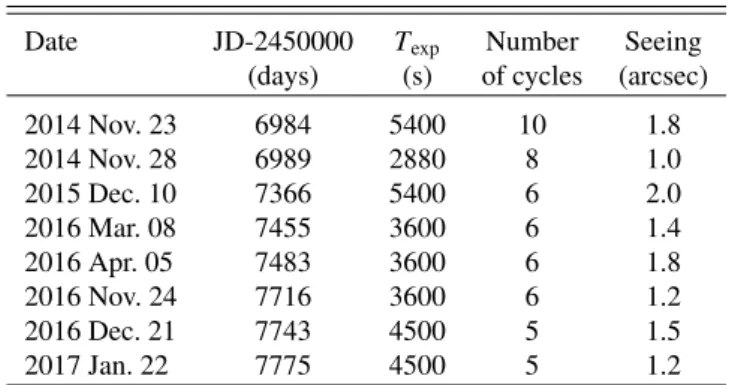
In the period from 2014 to 2017, we performed polarimetric observations of J1004+4112 at eight epochs. The log of obser-vations is given in Table2. The dichroic polarizer was used as
Table 2. Log of polarization observations of the lensed quasar J1004+4112 with the 6m telescope of SAO RAS.
Date JD-2450000 Texp Number Seeing
(days) (s) of cycles (arcsec)
2014 Nov. 23 6984 5400 10 1.8 2014 Nov. 28 6989 2880 8 1.0 2015 Dec. 10 7366 5400 6 2.0 2016 Mar. 08 7455 3600 6 1.4 2016 Apr. 05 7483 3600 6 1.8 2016 Nov. 24 7716 3600 6 1.2 2016 Dec. 21 7743 4500 5 1.5 2017 Jan. 22 7775 4500 5 1.2
a polarization analyzer. The polarization was measured with the method of Fesenkov. This method uses a series of observations at three fixed rotation angles of the analyzer: −60, 0, and+60◦.
The number of cycles, consisting of three consecutive frames at these angles, as well as the total exposure times are shown in Table2. Images were obtained in the photometric V band of the Johnson system. In Fig.1we mark three reference stars that we used for photometric calibration.
To find the zero-point of the polarization angle (PA), we observed the polarization standard HD 25443 (with p= 5.13% and PA= 134.2◦). The method of image-polarimetry, which accounts for the instrumental polarization, as well as atmospheric variability is describe inAfanasiev & Ipatov(2018), and here we do not repeat it in detail. We only briefly mention that we used a field of view 60× 60, covering around 50 stars, made histograms
of the Stokes parameters Q and U, and found their averaged val-ues as hQi= −0.15 ± 0.21 and hUi = 0.05 ± 0.17. The averaged Stokes parameters are the vector sum of the interstellar polar-ization in the direction of the Galactic longitude of b = 27.3◦.
To extract polarization of a lens component, we subtracted these averaged Stokes parameters from the observed U and Q of the lens component. The interstellar polarization in this direction is lower than p = 0.07% (seeHeiles 2000). This method yields results that show that the instrumental polarization is lower than p = 0.2% (seeAfanasiev & Ipatov 2018), which is taken into account in our measurements of the Q and U parameters.
Photometry of each lensed image was observed in the circle-like aperture with diameter of 400 centered at the image center with a spatial accuracy of about 0.1500. The flux measurements
were been on the local standard stars (denoted as stars 1–3 in Fig.1). The BVR fluxes of these stars were found using obser-vations of NGC 2420.
In the case of image polarimetry, which means differential measurements based on the photometric standards, the influ-ence of atmospheric extinction can be neglected. The atmo-spheric depolarization was taken into account using the method described inAfanasiev & Amirkhanyan(2012).
After measuring the intensities in the three angle-positions of the Polaroid – I(x, y)0, I(x, y)−60, and I(x, y)+60, we find the total
intensity I and normalized Stokes parameters Q and U at each point of the image with coordinates (x, y), using the following relationships:
I(x, y)= 2
3(I(x, y)0+ I(x, y)−60+ I(x, y)+60) Q(x, y)=2I(x, y)0− I(x, y)−60− I(x, y)+60
I(x, y)0+ I(x, y)−60+ I(x, y)+60
(1) U(x, y)= √ 3 2 I(x, y)+60− I(x, y)−60
I(x, y)0+ I(x, y)−60+ I(x, y)+60
The degree of polarization P and the polarization angle ϕ are calculated as P= pQ2+ U2, ϕ = ϕ slit− 1 2arctan U Q+ ϕ0. (2)
Here ϕslitis the angle of the vertical direction in the image and
ϕ0 is the zero-point, which was determined by observations of
polarization standards. The instrumental polarization and depo-larization of Earth’s atmosphere were taken into account using the method described inAfanasiev & Ipatov(2018).
3. Results
We took spectra of the four components in three epochs: 2007, 2008, and 2018. Additionally, we observed the polarization of the four images of J1004+4112 twice during 2014, four times in 2016, and one time in 2015 and 2017. We also compared our spectroscopic observations with those published earlier in 2003 (Inada et al. 2003).
3.1. Spectroscopic variability
When we compared the spectra obtained in the three epochs, we find a significant flux increase in the C IV blue line wing of com-ponent A (see Fig.2). This enhancement in the C IV blue wing was reported earlier by several authors (see, e.g.,Richards et al. 2004;Gómez-Álvarez et al. 2006;Green 2006;Motta et al. 2012;
Fian et al. 2018). The changes in the C IV line profile of the other three components were not significant. We only detect a change in the continuum level of component D, as shown in Fig.2. The continuum flux of component D was higher in 2007–2008 than in 2018. At these epochs, the conitnuum level of image D was similar to the continuum level observed in image B. However, in 2018 the continuum level was significantly lower in compo-nent D than in compocompo-nent C. This suggests that a significant microlensing event during 2007 and 2008 may have affected component D (see Fig. 2). Our error bars in the absolute flux measurements are estimated on the level 10–15%, therefore the observed changes in the D component continuum seem to be the real.
To explore changes in the line profiles, first we estimated the level of the continuum by fitting a cubic spline function through the windows that covered the following spectral ranges: around 3900 Å, 4600 Å, and 5400 Å. After this, the continuum was subtracted. The estimated error bars due to the continuum-subtraction procedure are at 3–4%. The C IV and CIII] lines were normalized to the line peaks and are presented in Fig.3.
A comparison of the normalized C IV line profiles of the four components observed in the three epochs (see the left panels in Fig.3) clearly shows a significant flux increase in the C IV blue wing only in component A. It is interesting to note that the red wing of the C IV line of component A is slightly smaller than in the other three components (see the first two left panels in Fig.3).
In the right panels of Fig.3we compare the CIII]λ1909 line profiles of the four components. They show that the CIII] line profiles of the different images are similar. Only in 2008 does the red wing of component D seem to be clearly higher (see the middle right panel in Fig.3), but an increase may also be present in 2018 (mostly in the lowest velocity fraction of the red wing). This enhancement may be caused by the microlensing event that is detected in the continuum (see Fig.2).
Inada et al.(2003) showed the first spectra with high signal-to-noise ratio (S/N) of SDSS J1004+4112 images that were observed with the Keck telescope. These spectra clearly show
Fig. 2.Spectra of the four components corresponding to three epochs: 2007 (bottom), 2008 (middle), and 2018 (top).
that the C IV line has an asymmetric profile with a different asymmetry in the different images (seeInada et al. 2003). This motivates us to measure the C IV asymmetry coefficient (γ) as (see, e.g.,Groeneveld & Meeden 1984)
γ = M3
M3/22 ,
where M2and M3are the second and third moments of the line
profiles. In Fig.4we show the measured asymmetries of the C IV lines for all four images.
To measure the C IV asymmetry, first we explored the influ-ence of different integration windows around the C IV line center. First we took a window of ±15.5 Å around the line center (which corresponds to a full width at half-maximum, FWHM, that is ∼31 Å or 6000 km s−1). This window includes about 80% of the total line flux, and we found that the asym-metry is −1.19 ± 0.08. Then we chose a larger window ±25.8 Å around the line center (in total 10 000 km s−1) that covered 95% of the total line flux, and found that in this case, the asymmetry is −1.01 ± 0.07. To avoid the influence of an absorption in the blue wing of C IV and a weak emission of He I (see Fig.3), we chose a wavelength interval ∼±25.8 Å around the line center to measure the asymmetry.
The second task was to determine the asymmetry and esti-mate the error bars of the C IV measured asymmetry. To do this, we performed the following procedure: (a) For each C IV line profile we estimated the error bars in the measured asymmetry using the bootstrap method (seeEfron 1979), that is, we first we
Fig. 3.C IV (left) and CIII] (right) emission line profiles of the four images in the three epochs: 2007 (bottom), 2008 (middle), and 2018 (top). produced a Monte Carlo random sample of asymmetry estimates
of the observed profiles by taking different (random) noises that contribute to the observed line profile errors; (b) After this, we constructed the histogram of the asymmetry where the averaged peak values were taken as the asymmetry and the histogram width as an estimated error of the asymmetry. Additionally, we estimated that the continuum subtraction contributes to the error bars by around 3–4%.
Figure3shows that the blue asymmetry of the A component can be clearly detected by comparing the line profiles. The red asymmetry in component D can also be detected, while compo-nents B and C seem to have a weaker and insignificant asymmetry. We tried to measure the CIII] asymmetry, but we found that the error bars are too high. We therefore cannot give any valid conclusion about CIII] asymmetry.
Figure4 shows that the A component has a blue asymme-try in all epochs. Additionally, we include the asymmeasymme-try coe ffi-cients corresponding to the observations in 2003 byInada et al.
(2003; first point in the plots of Fig. 4), and we found that in component A, the blue asymmetry of C IV in 2003 was weaker than in our observations. It is interesting to see that the C IV line in the component D has a red asymmetry that is more prominent in the 2018 observations (see also Fig.2).
To summarize, the main results of the spectroscopic obser-vations were the following:
– There is an enhancement of the blue wing of the C IV line of image A in all three epochs, with a maximum flux increase in the blue wing in 2008.
– The continuum flux of image D increased in the period of 2007–2008. In 2008, the CIII] red wing of image D also appears to be enhanced.
– The blue asymmetry of the C IV profile of the A component is present from 2003 to 2018, while component D seems to have a red asymmetry.
3.2. Polarization variability
The polarized light of J1004+4112 was observed in the period from 2014 to 2017 (see Table 2), covering eight epochs. In
Fig. 4.Asymmetry coefficients (see text) of the C IVλ1549 line profile,
obtained for each one of the four images at four epochs. The data cor-responding to 2003 are reproduced from the observations reported by
Inada et al.(2003).
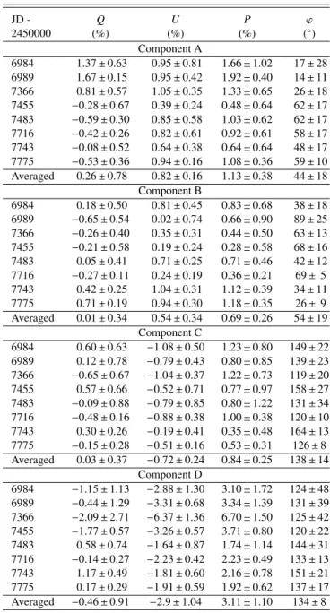
Figs.5and6we present the results. We also give our measure-ments of the polarization parameters (for all epochs and the aver-aged parameters) for the four components in Table3.
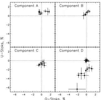
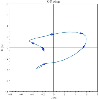
In Fig.5we present variations in the U and Q Stokes param-eters using the U Q-plane for all images. In the fourth plot (image D) we also show the observed U Q obtained for polarization zero standards (points with zero-zero position on the U Q-plane). The figure shows slight changes in the U Q plane for components A, B, and C, and strong changes can be seen in component D (off-centered points in the UQ plot of component D).
In Table3we list the observed polarization parameters (Q, U, p, and ϕ) for all epochs and their averaged values obtained in the period 2014–2017. The table shows (and also in Fig.5) that component A has an averaged location in the QU plane of hQi = 0.26 and hUi = 0.82 corresponding to an averaged
Fig. 5.U Q-plane plots for the four components of QSO J1004+4112.
Values of U Q for standard stars with zero polarization are plotted (points concentrated in the center, with zero-zero position) in the panel corresponding to image D, where off-centered points represent the change in U Q parameters of component D.
polarization angle of ϕ ∼ 40◦, which is slightly smaller than the
polarization angle in component B, and quite different than the angles in components C and D (hϕi ∼ 130◦).
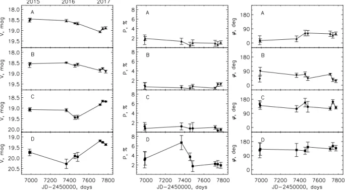
In Fig.6 we present the variability in the level of polariza-tion (p) and the polarizapolariza-tion angle (ϕ) during the period 2014– 2017: we plot changes in the V magnitude (first panel), the level of polarization in percent (second panel), and the polarization angle (third panel). Small changes in the magnitude of compo-nents A and B are evident, as are changes in the polarization parameters (p and ϕ). A strong change in the magnitude and in the polarization parameters is detected in component D. Com-ponents A, B, and C show polarization between 0.5% and 2%, as expected for type 1 AGNs. The expected level of polarization in type 1 AGNs is ≤1% (see, e.g.,Smith et al. 2004;Afanasiev et al. 2019). While component D shows a higher variability in the level of polarization in the first three epochs (between 3% and 7%). In this period, we also detect flux variability in image D (see the first panel in Fig.6).
As a summary of the polarization observations, we can out-line the following results:
– The averaged polarization parameters for the four images of J1004+4112 are different in each image.
– Changes in the polarization parameters of components A, B, and C are not significant, but component D shows a strong change in the polarization parameters during the 2014–2017 period. Image D shows a higher level of polarization and change in polarization, which is correlated with the change in brightness. – The averaged polarization angles (see Table3) are different for different components: components A and B seem to have polarization angles of ∼40–50◦, while components C and D have polarization angles of ∼130◦.
4. Discussion and interpretation of the observations
The nature of observed spectroscopic (and polarometric) vari-ability of an image in a lensed system can be due to intrinsic variability (which is often observed in non-lensed quasars) and
microlensing. Before we discuss and interpret the observed vari-ability in the J1004+4112 lens system, we therefore clarify the nature of the observed variability.
Time-delay measurements between the J1004+4112 images show a short time delay between components A and B (B leads A by ∼40 days, seeFohlmeister et al. 2007,2008), which is very close to the theoretical predictions (∼30 days, seeRichards et al. 2004). The time delay between image C and A is about 820 days (C leads A), and it is longer between image A and D (D lags A by >1250 days, seeFohlmeister et al. 2008). The similarity between the CIII] profiles for B and C suggests that a change in the line shape of image D (see Fig.3, larger red wing in 2008) caused by intrinsic variability is unlikely because the time delay between B and C is longer than two years. When we compare the contiuum variablilty in Fig. 2, significant variability is seen in compo-nent D (e.g., between May 2007 and October 2008, without any amplification in the C component). Moreover,Fian et al.(2018) showed that in the period 2007–2010, component D showed high variability that is caused by gravitational microlensing (see their Fig. 4 and the corresponding discussion in the paper). Especially in the period 2007–2008, the variability of component D was caused by microlensing, as was shown inFian et al.(2018).
On the other hand, the polarization variability in component D strongly changed by about 4–5% (see Fig. 6 and Table 3), which is too high to be expected from the intrinsic polarization variability of AGNs (which is around 1%; see, e.g., Afanasiev et al. 2014, 2015; Kokubo 2016; Koshida et al. 2017). The continuum intrinsic variability in polarization of type 1 AGNs is probably caused by the change in the accretion disk polar-ization (see Kokubo 2016), and it is not expected to change significantly (below 1–2%). The maximum contribution of the accretion disk polarization through rediative transfer is about 10% (Chandrasekhar 1950), but as a rule, this is lower in type 1 AGNs at about 0.5–1%. A strong change in polarization in com-ponent D alone (during the 2014–2017 period) is also unlikely due to intrinsic polarization variability.
We cannot absolutely rule out a contribution of the intrin-sic variability to the observed variability of component D, but it seems that in the observed period where variability in polar-ization is present, variability caused by microlensing is domi-nant. Therefore we consider microlensing in this section as the main cause of the observed variability in flux magnification (and polarization) of component D and of the blue line wing amplifi-cation in component A.
4.1. Spectroscopic variability
The detected change in the blue wing of C IV was also reported in previous papers (seeRichards et al. 2004;Green 2006;Lamer et al. 2006;Motta et al. 2012;Fian et al. 2018, etc.). To explain the exclusive amplification of the C IV blue wing in image A (without a similar amplification in the CIII] line of A), we point out two observational facts: (a) The amplification in the C IV blue wing of component A is not followed by the amplifica-tion of the center and/or red wing of the line (as expected in the case of a classical disk-like BLR; see, e.g.,Popovi´c et al. 2001a) or by a magnification of the A image continuum (nei-ther has it been detected in previous observations; seeRichards et al. 2004;Green 2006;Lamer et al. 2006;Motta et al. 2012). We only detect a significant continuum amplification in com-ponent D during the first two epochs (see Fig.2); (b) In Fig.3
the C IV red wing of component A appears smaller than the red wings of the other components (especially compared with the red wings of components D and C). This can be a consequence of the
Fig. 6.Variability in the magnitude (left), polarization (middle), and polarization angle (right) for all four components.
normalization to the line maximum if some additional emission contributes to the blue wing and core of the C IV line of image A but not to the red wing (see Fig.3).
To explain these facts, a physical scenario might be consid-ered in which microlensing can magnify only a part of the broad emission lines (see, e.g.,Popovi´c et al. 2001a;Abajas et al. 2002,
2007). The C IV BLR dimensions can be estimated using the luminosity of the C IV line and nearby continuum (at λ1350 Å; see, e.g.,Kong et al. 2006;Kaspi et al. 2007;Trevese et al. 2014;
Lira et al. 2018;Hoormann et al. 2019). To estimate a continuum at λ1350 Å that is not amplified, we first calculated the amplifi-cation (A) for each component using (seeWambsganss 1998)
A= 1
[(1 − κ)2−γ2], (3)
where κ and γ for each component were taken fromFian et al.
(2016). The obtained amplification is A = 18.36 (for A), 7.76 (for B), 3.62 (for C), and 1.6 (for D). We measured the fluxes of all four components from observations performed in 2018 because the S/N was best for observations in this epoch. The obtained unlensed luminosities (taking standard cosmological parameters) for the components at 1350 are ∼5.1 × 1044erg s−1 (for A), 7.3 × 1044erg s−1(for B), 7.9 × 1044erg s−1(for C), and
7.3 × 1044 (for D), which gives an averaged non-lensed quasar luminosity of λL(1350) = (6.9 ± 0.9) × 1044erg s−1. Using the
R–L relation fromKong et al.(2006), we obtained that the C IV BLR dimension is ∼42 light days, and using the R–L relations for luminous quasars given byKaspi et al.(2007) andLira et al.
(2018), we obtained a smaller C IV BLR dimension of ∼15– 20 light days. The estimated C IV BLR dimension from the C IV line luminosity using the relation given in Kong et al.(2006) (Eq. (2) given in the paper) is significantly larger than the one estimated from the continuum. The reverberation relations given in Kaspi et al.(2007) and Lira et al.(2018) were derived for high-luminosity quasars, therefore they give some minimum val-ues of the C IV BLR. The estimated accretion disk dimension in SDSS J1004+4112 is ∼9 light days (Fian et al. 2016), which
implies that the BLR is at least several times larger than accretion disk. Therefore, the C IV BLR dimension in SDSS J1004+4112 probably is more than some dozen light days.
The microlensing Einstein ring radius (ERR) for J1004+4112 can be calculated as (Fian et al. 2016)
ERR= 9 l. days · s
M 0.3 M
l. days,
which gives around 9 l. days for a 0.3 solar mass microlens that is assumed to be present in the SDSS J1004+4112 lens system. When we compare the ERR dimensions with the esti-mated dimensions of the BLR, we cannot expect a significant microlensing magnification of the broad emission lines in this system (see Abajas et al. 2002) because the ERR is at least twice smaller than the C IV BLR estimated dimension. More-over, the variation in the blue wing of component A seems to occur in a relative short time (seeRichards et al. 2004), there-fore microlensing of the whole BLR can be excluded.
As we noted above, the C IV line shapes of non-lensed quasars show a blue asymmetry and/or shift (see, e.g.,Richards et al. 2011; Marziani et al. 2019) that indicates an out-flow contribution to the C IV broad line fluxes. In principle, different C IV BLR geometries can be considered (spherical, disk-like, outflowing, etc.), but there may be a stratification in the BLR where one component is disk-like (follows the accretion disk kine-matics) and an additional component that originates in an outflow (see Fig.7).
To explain the amplification in the blue wing of component A, we considered a phenomenological model as shown in the left panel of Fig.7. The scale in the panel is given in arbitrary units. The map and scheme of the C IV-emitting region shown in Fig.7are only an illustration in order to qualitatively explain the C IV blue wing amplification. Because we found that the C IV BLR probably has larger dimensions (about 40 light days) than the projected microlens ERR (about 9 light days), the amplifica-tion is probably not due to microlensing of the whole disk-like BLR. The illustration of the disk is shown in the left panel, which
Table 3. Polarization parameters for the four components of the gravita-tional lens J1004+4112 observed in different epochs and their averaged values for the period 2014–2017.
JD - Q U P ϕ 2450000 (%) (%) (%) (◦) Component A 6984 1.37 ± 0.63 0.95 ± 0.81 1.66 ± 1.02 17 ± 28 6989 1.67 ± 0.15 0.95 ± 0.42 1.92 ± 0.40 14 ± 11 7366 0.81 ± 0.57 1.05 ± 0.35 1.33 ± 0.65 26 ± 18 7455 −0.28 ± 0.67 0.39 ± 0.24 0.48 ± 0.64 62 ± 17 7483 −0.59 ± 0.30 0.85 ± 0.58 1.03 ± 0.62 62 ± 17 7716 −0.42 ± 0.26 0.82 ± 0.61 0.92 ± 0.61 58 ± 17 7743 −0.08 ± 0.52 0.64 ± 0.38 0.64 ± 0.64 48 ± 17 7775 −0.53 ± 0.36 0.94 ± 0.16 1.08 ± 0.36 59 ± 10 Averaged 0.26 ± 0.78 0.82 ± 0.16 1.13 ± 0.38 44 ± 18 Component B 6984 0.18 ± 0.50 0.81 ± 0.45 0.83 ± 0.68 38 ± 18 6989 −0.65 ± 0.54 0.02 ± 0.74 0.66 ± 0.90 89 ± 25 7366 −0.26 ± 0.40 0.35 ± 0.31 0.44 ± 0.50 63 ± 13 7455 −0.21 ± 0.58 0.19 ± 0.24 0.28 ± 0.58 68 ± 16 7483 0.05 ± 0.41 0.71 ± 0.25 0.71 ± 0.46 42 ± 12 7716 −0.27 ± 0.11 0.24 ± 0.19 0.36 ± 0.21 69 ± 5 7743 0.42 ± 0.25 1.04 ± 0.31 1.12 ± 0.39 34 ± 11 7775 0.71 ± 0.19 0.94 ± 0.30 1.18 ± 0.35 26 ± 9 Averaged 0.01 ± 0.34 0.54 ± 0.34 0.69 ± 0.26 54 ± 19 Component C 6984 0.60 ± 0.63 −1.08 ± 0.50 1.23 ± 0.80 149 ± 22 6989 0.12 ± 0.78 −0.79 ± 0.43 0.80 ± 0.85 139 ± 23 7366 −0.65 ± 0.67 −1.04 ± 0.37 1.22 ± 0.73 119 ± 20 7455 0.57 ± 0.66 −0.52 ± 0.71 0.77 ± 0.97 158 ± 27 7483 −0.09 ± 0.88 −0.79 ± 0.85 0.80 ± 1.22 131 ± 34 7716 −0.48 ± 0.16 −0.88 ± 0.38 1.00 ± 0.38 120 ± 10 7743 0.30 ± 0.26 −0.19 ± 0.41 0.35 ± 0.48 164 ± 13 7775 −0.15 ± 0.28 −0.51 ± 0.16 0.53 ± 0.31 126 ± 8 Averaged 0.03 ± 0.37 −0.72 ± 0.24 0.84 ± 0.25 138 ± 14 Component D 6984 −1.15 ± 1.13 −2.88 ± 1.30 3.10 ± 1.72 124 ± 48 6989 −0.44 ± 1.29 −3.31 ± 0.68 3.34 ± 1.39 131 ± 39 7366 −2.09 ± 2.71 −6.37 ± 1.36 6.70 ± 1.50 125 ± 42 7455 −1.77 ± 0.57 −3.26 ± 0.57 3.71 ± 0.80 120 ± 22 7483 0.58 ± 0.74 −1.64 ± 0.87 1.74 ± 1.14 144 ± 31 7716 −0.14 ± 0.27 −2.23 ± 0.42 2.23 ± 0.49 133 ± 13 7743 1.17 ± 0.49 −1.81 ± 0.60 2.16 ± 0.78 151 ± 21 7775 0.17 ± 0.29 −1.91 ± 0.59 1.92 ± 0.62 137 ± 17 Averaged −0.46 ± 0.91 −2.9 ± 1.04 3.11 ± 1.10 134 ± 8
emits an emission line (illustrated as the dashed line in the right panel).
There may be a large caustic (shown in the left panel) that slowly crosses the blue part, slightly magnifying the blue wing (the solid line in the right panel). Additionally, the caustic may also microlens the compact part of the emission that comes from the outflowing component (illustrated as a small dashed line in the blue wing; see the right panel), whichmay vary in a short period. This scenario can provide an explanation of the fast variability in the part of the blue wing only in component A. On the other hand, this can also explain the relatively low intensity of the red wing that is observed in component A with respect to component B.
As we noted above, the HST image of SDSS J1004+4112 shows a point-like object close to image A (Sharon et al. 2005) that may be the source of the spurious emission that contam-inates the blue wing of C IV. However, it is hard to explain the nature of an object with a spectral energy distribution that
Fig. 7.Scheme of the caustic crossing of the compact jet-like region (left) that emits a small contribution to the blue wing of the C IVλ1550 line of QSO J1004+4112 (right). The dimension scale on the left panel is given in arbitrary units, where the disk-like BLR is assumed to be several tens of light days (see text) and the jet-like region is assumed to more compact (<9 light days) to be microlensed.
has a short-wavelength interval that only contributes to the blue C IV wing intensity. Additionally, we cannot see any contribu-tion to the other lines or addicontribu-tional continuum in the spectrum of image A that shows simultaneous change with the changes in the C IV blue wing. This means that this object probably does not contribute significantly to the blue wing amplification of image A.
Finally, we comment on the less outstanding but signifi-cant enhancement of the red wing of image D, which may also be related to microlensing. This hypothesis is supported by the presence of microlensing magnification in the continuum of image D.
4.2. Microlensing of the scattering region of the torus Assuming that the lensed source has a complex polarization struc-ture, the image polarization can also be expected to be different. Theoretically, several papers have considered the polarization due to the macro- and microlensing (see, e.g.,Schneider & Wagoner 1987;Bogdanov et al. 1996). Observational microlensing effects in the broadband and spectra of the lensed quasar H1413+117were observed (seeChae et al. 2001;Hutsemékers et al. 2015). In this system, component D showed a higher level of polarization and polarization angle.
The polarization sources in lensed quasars can have a di ffer-ent nature. Based on some observational facts, we expect polar or equatorial scattering to be the main polarization mechanisms in AGNs, with polar scattering dominant in type 2 objects and equatorial scattering in type 1 objects (see, e.g., Smith et al. 2004;Afanasiev & Popovi´c 2015; Popovi´c et al. 2018). In all images of J1004+4112, broad Lyα, C IV, and CIII] lines are observed (see our spectra, as well as those inInada et al. 2003;
Richards et al. 2004;Green 2006;Lamer et al. 2006;Motta et al. 2012;Fian et al. 2016). Thus, because SDSS J1004+4112 is a type 1 AGN, we consider equatorial scattering as the dominant polarization mechanism.
4.2.1. Expected polarization variability during a microlensing event
As we noted above, variability is observed in the polariza-tion parameters of all components (see Figs.5 and6), but the most prominent variability is observed in component D. The
change in polarization correlates with the change in the magni-tude of component D, therefore we expect that the microlensing effect can affect the polarization parameters (Stokes parameters, and consequently, the level of polarization and the polarization angle). In order to demonstrate the influence of microlensing on the polarization parameters, we studied the microlensing effect in the scattering region that is assumed to be located in the inner part of the torus.
To have a realistic model of polarization in AGN, we mod-eled the equatorial scattering using the Monte Carlo radiative transfer code
stokes
(assuming type 1 AGNs, see more details inGoosmann & Gaskell 2007; Marin et al. 2015; Savi´c et al. 2018, etc.). For the torus we considered a flared-disk geome-try assuming Thomson scattering in the inner part of the torus. The inner radius of the torus was taken as 0.1 pc (∼13 ERR, see Appendix A), assuming an optical depth of τ = 5, and the outer radius of the torus scattering region is 0.2 pc (∼26 ERR). The Stokes parameters were calculated across the entire scattering region (for more details, see AppendixA.1, see also Fig.A.2). We assumed a face-on torus orientation (with respect to an observer), therefore the level of polarization was very low, ∼0.2% of the not microlensed torus.The polarization rate and angle across the scattering region show a significant gradient. The change in polarization parame-ters can be detected in the interval of 0.01 pc ≈ 12 l.d., which is comparable with an ERR of a star with 0.3 M (∼9 l.d.).
Additionally, we generated a microlensing map for image D, taking the estimates for convergence and shear given inFian et al.(2016). The dimensions of the map are 4000 × 4000 l.d.2,
with a resolution of 1 light day (1 pix= 1 l.d.), which is equiva-lent to 241.6 × 241.6 ERR2.
This map was convoluted with the Q and U Stokes param-eter maps, which have dimensions 476 × 476 l.d., with the same resolution 1 pix= 1 l.d. After convolving the Stokes parameters with the microlensing map, we calculated p and ϕ for each pixel according to Eq. (A.2). Figure8is a zoom-in of the larger polar-ization map obtained after convolution. A detailed description of our simulations is given in AppendixA.
To gain an impression of the timescale, we converted the polarization level and angle maps into the standard timescale using (seeTreyer & Wambsganss 2004;Jovanovi´c et al. 2008) tE ≈ (1+ zl)
ERR v⊥
,
where ERR is the point-like ERR projected onto the source plane, v⊥ is the relative transverse velocity that is typically
v⊥ ∼ 600 km s−1 (see Treyer & Wambsganss 2004), and zl is
the cosmological redshift of the lens.
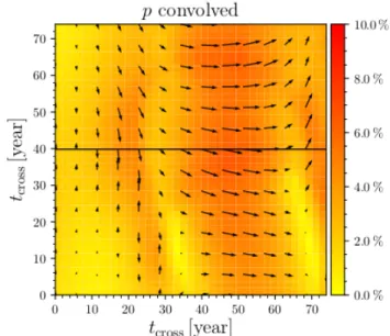
In Fig.8 we present the magnification map corresponding to the polarization rate and polarization angle. The solid line in Fig.8represents the source path across the map, which results in the change of parameters that is shown in Fig.9. The first plot in Fig.9 presents the change in intensity due to microlensing. The total intensity accounts for the radiation of the point source plus the radiation scattered off the torus. The second plot shows the change in the polarization (that can be from 2% to 6%), and the third plot shows the change in polarization angle. Figure9
shows that the observed polarization of component D can be qualitatively described by the model, and the polarization level and the angle of polarization can change significantly during a microlensing event. Additionally, in some cases, microlensing can strongly increase the polarization rate (by a factor 10, see Fig. 9). However, using our model and calculating the proba-bly density function for the polarization rate (see Fig.A.4, right
Fig. 8. Magnification map (see Appendix A) showing the effect of
microlensing on the degree of polarization p (given in color) and on the polarization angle ϕ (arrows). The level of polarization is given in percent. Arrows paralell to the Y-axis correspond to ϕ = 0, and the arrow length corresponds to the p value. The solid black line represents the path of the source, starting from left to right. This map is a subregion of a much larger magnification map shown in AppendixA.
middle and bottom panels), we found that our model (microlens and source) gives that the most probable microlens rate is about 1%, and has a relatively high probability until 4%. This agrees with the observed polarization variability in component D.
In Fig. 10we present the variability in the U Q plane. The changes in the U Q plane can be significant during a microlens-ing event. Consequently, the polarization angle can change from 0 to 180◦ and the level of polarization can reach 10%. In our simulation we did not see any significant correlation between the change in polarization angle and the polarization level. The amplification in intensity coincides with the change in polar-ization parameters, but the correlation between the behavior of these changes is not significant (i.e., the maximum intensity does not correspond with the maximum polarization level, etc.).
The difference between polarization angle of image C is very different from the polarization angle observed in images A and B. This difference may be also due to microlensing, but at the beginning of microlensing, without any sign of a strong change in polarization degree. Figure9shows that the changes in polar-ization angle can be strong (third panel of Fig.9) without strong changes in polarization rate (middle panel of Fig.9). However, this needs to be confirmed by future observations in polarized light of this component.
4.2.2. Effect of macrolensing on image polarization
We also explored the possibility that the different locations in the QU plane of the averaged polarization values for the different images were caused by macrolensing through a different trans-formation of the source. To do this study we fit a simple SIS+γe model to the positions of the four images of J1004+4112. As far as images A and B are relatively close (in fact in near infrared observations taken with the HST it can be seen that for enough large sources the images merge into one arc) we can think that the central position of the source is not far away from a macro-caustic. We apply this model to the 2D distributions of
Fig. 9. Modeled changes in intensity (up), degree of polarization p (middle), and polarization angle ϕ (bottom) corresponding to the cross-ing path shown as a solid line in Fig.8.
Qand U Stokes parameters of the torus described in Sect.4.2.1
to compute their lensed images and to calculatethe histogram of polarizations for the four images. In the case of the detached C and D images, we find no differences with respect to the source histogram. That is, in images C and D, the polarization changes cannot be attributed to macrolensing. This result seems easy to explain. Lensing acts like a linear transformation in a region in space if its size is small enough. The source is very small (0.05 mas, according to the torus dimensions described in Sect. 4.2.1) and each surface element is transformed under the same linear transformation, therefore the source histogram does not change under macrolensing. In the case of images A and B, which appear merged in the near-infrared, the situation may be different. If the source is large enough to be crossed by a caustic (a possibility, although the torus is so small that it seems unlikely, but not impossible because the location of the source with respect to the caustic depends on the lens models), lens-ing will produce two images of the whole source and two addi-tional images of only the inner part of the caustic part of the source. Under these circumstances, macrolensing could change
Fig. 10.Variation in Stokes parameters Q and U along the crossing path defined in Fig.8. Arrows denote the direction in which Q and U evolve as the source crosses the path on the microlening map, starting from left to right.
polarization. However, A and B show no significant differences in the QU plane. Thus, there is no reasons to assume that the caustic intersects the torus, confirming that it is far smaller than the source that causes the near-infrared arcs. Microlensing con-sequently is a more plausible explanation for the relative shifts between images in the QU plane.
5. Conclusions
We presented spectroscopic and polarimetric observations of the lensed quasar J1004+4112 obtained with the 6 m telescope of SAO RAS. We analyzed the observed spectra, and the C IV blue line bump in component A may be explained with a phe-nomenological model for the BLR that includes an outflowing component. Additionally, we studied the effect of macro- and microlensing on the polarized light caused by Thomson scatter-ing in the inner part of the torus. Based on our analysis, we can outline the following conclusions:
– The C IV blue bump seen only in image A that has been reported in earlier observations is also present in the three epochs (2007, 2008, and 2018) of our observations. The CIII] line pro-file of image A is similar to the line propro-files observed in the other three images. To explain this effect, we propose that the outflow contributes to the blue wing. When we assume that the C IV BLR is about several dozen light days, the outflowing region should be more compact (several light days) in order to be microlensed by a microlens ERR of ∼9 light days, as estimated for the SDSS J1004+4112 lens system.
– We observed the polarized light of J1004+4112. We find that the averaged positions on the U Q-plane of the different images are different. Components A and B have an average polarization angle of about 40–50◦, while the C and D compo-nents have an averaged polarization angle of about 140◦. The relatively small size of the torus makes an explanation of these differences related to macrolensing unlikely, which basically acts like a linear transformation of the source.
– Significant variability of the polarization is observed only in component D. Simulation of the microlensing of a scatter-ing region in the inner part of the torus can qualitatively explain the observed changes in the U Q-plane, as well as the change in polarization level and the polarization angle of image D observed in the 2014–2017 period.
Additionally, we presented a qualitative model of microlens-ing of a disk-like plus emittmicrolens-ing outflow BLR to explain the observed magnification of the C IV blue wing of component A. This needs to be confirmed in future spectroscopic observations.
Acknowledgements. This work is supported by the Ministry of Education, Science and Technological Development of R. Serbia (the project 146001: “Astrophysical Spectroscopy of Extragalactic Objects”) and Russian Foundation for Basic Research (grant No. 19-32500). The observations at the SAO RAS 6 m telescope were carried out with the financial support of the Ministry of Science and Higher Education of the Russian Federation. Dj. Savi´c thanks the RFBR for the realization of the three months short term scientific visit at SAO funded by the grant 19-32-50009. We would like to thank to the referee for very useful comments.
References
Abajas, C., Mediavilla, E., Muñoz, J. A., Popovi´c, L. ˇC., & Oscoz, A. 2002,ApJ, 576, 640
Abajas, C., Mediavilla, E., Muñoz, J. A., Gómez-Alvarez, P., & Gil-Merino, R. 2007,ApJ, 658, 748
Afanasiev, V. L., & Amirkhanyan, V. R. 2012,Astrophys. Bull., 67, 438 Afanasiev, V. L., & Ipatov, A. V. 2018,Astrophys. Bull., 73, 241 Afanasiev, V. L., & Moiseev, A. V. 2005,Astron. Lett., 31, 194 Afanasiev, V. L., & Moiseev, A. V. 2011,Baltic Astron., 20, 363 Afanasiev, V. L., & Popovi´c, L. ˇC. 2015,ApJ, 800, L35
Afanasiev, V. L., Dodonov, S. N., & Moiseev, A. V. 2001, in Proc. Int. Conf. Stellar Dynamics: from Classic to Modern. Sobolev Astron. Inst. St Petersburg, eds. L. L. Ossipkov, & I. I. Nikiforov, 103
Afanasiev, V. L., Popovi´c, L. ˇC., Shapovalova, A. I., Borisov, N. V., & Ili´c, D. 2014,MNRAS, 440, 519
Afanasiev, V. L., Shapovalova, A. I., Popovi´c, L. ˇC., & Borisov, N. V. 2015, MNRAS, 448, 2879
Afanasiev, V. L., Popovi´c, L. ˇC., & Shapovalova, A. I. 2019,MNRAS, 482, 4985 Belle, K. E., & Lewis, G. F. 2000,PASP, 112, 320
Blackburne, J. A., Pooley, D., Rappaport, S., & Schechter, P. L. 2011,ApJ, 729, 34
Bogdanov, M. B., Cherepashchuk, A. M., & Sazhin, M. V. 1996,Ap&SS, 235, 219
Braibant, L., Hutsemékers, D., Sluse, D., & Goosmann, R. 2017,A&A, 607, A32 Chae, K.-H., Turnshek, D. A., Schulte-Ladbeck, R. E., Rao, S. M., & Lupie,
O. L. 2001,ApJ, 561, 653
Chandrasekhar, S. 1950,Radiative Transfer(Oxford: Clarendon Press) Chartas, G., Agol, E., Eracleous, M., et al. 2002,ApJ, 568, 509 Chartas, G., Kochanek, C. S., Dai, X., et al. 2012,ApJ, 757, 137 Chartas, G., Krawczynski, H., Zalesky, L., et al. 2017,ApJ, 837, 26 Chen, B., Dai, X., Baron, E., & Kantowski, R. 2013,ApJ, 769, 131
Dai, X., Chartas, G., Agol, E., Bautz, M. W., & Garmire, G. P. 2003,ApJ, 589, 100
Dai, X., Chartas, G., Eracleous, M., & Garmire, G. P. 2004,ApJ, 605, 45 Donnarumma, I., De Rosa, A., Vittorini, V., et al. 2011,ApJ, 736, L30 Efron, B. 1979,Ann. Stat., 7, 1
Fian, C., Mediavilla, E., Hanslmeier, A., et al. 2016,ApJ, 830, 149 Fian, C., Guerras, E., Mediavilla, E., et al. 2018,ApJ, 859, 50 Fohlmeister, J., Kochanek, C. S., Falco, E. E., et al. 2007,ApJ, 662, 62 Fohlmeister, J., Kochanek, C. S., Falco, E. E., Morgan, C. W., & Wambsganss,
J. 2008,ApJ, 676, 761
Gómez-Álvarez, P., Mediavilla, E., Muñoz, J. A., et al. 2006,ApJ, 645, L5 Goosmann, R. W., & Gaskell, C. M. 2007,A&A, 465, 129
Green, P. J. 2006,ApJ, 644, 733
Groeneveld, R. A., & Meeden, G. 1984,The Statistician, 33, 391 Guerras, E., Mediavilla, E., Jimenez-Vicente, J., et al. 2013,ApJ, 764, 160 Heiles, C. 2000,ApJ, 119, 923
Hales, C. A., & Lewis, G. F. 2007,PASA, 24, 30
Hoormann, J. K., Martini, P., Davis, T. M., et al. 2019,MNRAS, 487, 3650 Hutsemékers, D., Lamy, H., & Remy, M. 1998,A&A, 340, 371
Hutsemékers, D., Sluse, D., Braibant, L., & Anguita, T. 2015,A&A, 584, A61 Hutsemékers, D., Braibant, L., Sluse, D., Anguita, T., & Goosmann, R. 2017,
Front. Astron. Space Sci., 4, 18
Inada, N., Oguri, M., Pindor, B., et al. 2003,Nature, 426, 810
Jiménez-Vicente, J., Mediavilla, E., Kochanek, C. S., et al. 2014,ApJ, 783, 47 Jovanovi´c, P., Zakharov, A. F., Popovi´c, L. ˇC., & Petrovi´c, T. 2008,MNRAS,
386, 397
Kartasheva, T. A., & Chunakova, N. M. 1978,Astrofizicheskie Issledovaniia Izvestiya Spetsial’noj Astrofizicheskoj Observatorii, 10, 44
Kaspi, S., Brandt, W. N., Maoz, D., et al. 2007,ApJ, 659, 997 Kishimoto, M., Hönig, S. F., Antonucci, R., et al. 2011,A&A, 536, A78 Kokubo, M. 2016,PASJ, 68, 52
Kokubo, M. 2017,MNRAS, 467, 3723
Kong, M.-Z., Wu, X.-B., Wang, R., & Han, J.-L. 2006, Chin. J. Astron. Astrophys., 6, 396
Koshida, S., Minezaki, T., Yoshii, Y., et al. 2014,ApJ, 788, 159 Koshida, S., Yoshii, Y., Kobayashi, Y., et al. 2017,ApJ, 842, L13 Krawczynski, H., & Chartas, G. 2017,ApJ, 843, 118
Lamer, G., Schwope, A., Wisotzki, L., & Christensen, L. 2006,A&A, 454, 493 Lira, P., Kaspi, S., Netzer, H., et al. 2018,ApJ, 865, 56
MacLeod, C. L., Jones, R., Agol, E., & Kochanek, C. S. 2013,ApJ, 773, 35 Marin, F., Goosmann, R. W., & Gaskell, C. M. 2015,A&A, 577, A66 Marziani, P., del Olmo, A., Martínez-Carballo, M. A., et al. 2019,A&A, 627,
A88
Mathis, J. S., Rumpl, W., & Nordsieck, K. H. 1977,ApJ, 217, 425 Mediavilla, E., Muñoz, J. A., Lopez, P. et al. 2006,ApJ, 653, 942 Mediavilla, E., Muñoz, J. A., Falco, E., et al. 2009,ApJ, 706, 1451 Mediavilla, E., Mediavilla, T., Muñoz, J. A., et al. 2011,ApJ, 741, 42 Mediavilla, E., Jiménez-Vicente, J., Fian, C., et al. 2018,ApJ, 862, 104 Motta, V., Mediavilla, E., Falco, E., & Muñoz, J. A. 2012,ApJ, 755, 82 Neronov, A., Vovk, I., & Malyshev, D. 2015,Nat. Phys., 11, 664 Netzer, H. 2015,ARA&A, 53, 365
Oguri, M., Inada, N., Keeton, C., et al. 2004,ApJ, 605, 78 Ota, N., Inada, N., Oguri, M., et al. 2006,ApJ, 647, 215 Peterson, B. M. 2014,Space Sci. Rev., 183, 253 Popovi´c, L. ˇC., & Chartas, G. 2005,MNRAS, 357, 135
Popovi´c, L. ˇC., Mediavilla, E. G., & Muõz, J. A. 2001a,A&A, 378, 295 Popovi´c, L. ˇC., Mediavilla, E. G., Muñoz, J. A., Dimitrijevi´c, M. S., & Jovanovi´c,
P. 2001b,Serb. Astron. J., 164, 53
Popovi´c, L. ˇC., Mediavilla, E. G., Jovanovi´c, P., & Muñoz, J. A. 2003,A&A, 398, 975
Popovi´c, L. ˇC., Jovanovi´c, P., Mediavilla, E., et al. 2006,ApJ, 637, 620 Popovi´c, L. ˇC., Afanasiev, V. L., & Shapovalova, A. I. 2018,Revisiting
Narrow-line Seyfert 1 Galaxies and Their Place in the Universe. 9-13 April 2018.
Padova Botanical Garden, Italy, PoS(NLS1-2018)001 Online athttps://
pos.sissa.it/cgi-bin/reader/conf.cgi?confid=328, 1
Richards, G. T., Keeton, C. R., Pindor, B., et al. 2004,ApJ, 610, 679
Richards, G. T., Kruczek, N. E., Gallagher, S. C., et al. 2011, AJ, 141, 167
Rojas Lobos, P. A., Goosmann, R. W., Marin, F., & Savi´c, D. 2018,A&A, 611, A39
Savi´c, D., Goosmann, R., Popovi´c, L. ˇC., Marin, F., & Afanasiev, V. L. 2018, A&A, 614, A120
Schneider, P., & Wagoner, R. V. 1987,ApJ, 314, 154
Sharon, K., Ofek, E. O., Smith, G. P., et al. 2005,ApJ, 629, L73
Sluse, D., Claeskens, J.-F., Hutsemékers, D., & Surdej, J. 2007,A&A, 468, 885
Sluse, D., Hutsemékers, D., Courbin, F., Meylan, G., & Wambsganss, J. 2012, A&A, 544, A62
Sluse, D., Kishimoto, M., Anguita, T., Wucknitz, O., & Wambsganss, J. 2013, A&A, 553, A53
Smirnova, A. A., Gavrilovi´c, N., Moiseev, A. V., et al. 2007,MNRAS, 377, 480
Smith, J. E., Robinson, A., Alexander, D. M., et al. 2004,MNRAS, 350, 140 Stalevski, M., Fritz, J., Baes, M., Nakos, T., & Popovi´c, L. ˇC. 2012a,MNRAS,
420, 2756
Stalevski, M., Jovanovi´c, P., Popovi´c, L. ˇC., & Baes, M. 2012b,MNRAS, 425, 1576
Stalevski, M., Tristram, K. R. W., & Asmus, D. 2019,MNRAS, 484, 3334 Suganuma, M., Yoshii, Y., Kobayashi, Y., et al. 2006,ApJ, 639, 46
Torres, D. F., Romero, G. E., Eiroa, E. F., Wambsganss, J., & Pessah, M. E. 2003, MNRAS, 339, 335
Trevese, D., Perna, M., Vagnetti, F., Saturni, F. G., & Dadina, M. 2014,ApJ, 795, 164
Treyer, M., & Wambsganss, J. 2004,A&A, 416, 19
Vives-Arias, H., Muñoz, J. A., Kochanek, C. S., Mediavilla, E., & Jiménez-Vicente, J. 2016,ApJ, 831, 43
Vovk, I., & Neronov, A. 2016,A&A, 586, A150 Wambsganss, J. 1992,ApJ, 386, 19
Wambsganss, J. 1998,Liv. Rev. Relativ., 1, 12 Williams, L. L. R., & Saha, P. 2004,AJ, 128, 2631
Appendix A: Microlensing of an equatorial scattering region in AGN
Characteristic polarization in type 1 AGNs is caused by equa-torial scattering in the innermost part of the torus (seePopovi´c et al. 2018). Therefore, here we consider microlensing of the equatorial scattering region, which is assumed to be located in the inner part of the torus.
A.1. Modeling polarization: equatorial scattering in the torus To simulate the equatorial scattering in the inner part of torus, we applied the 3D Monte Carlo radiative transfer code
stokes
of Goosmann & Gaskell (2007). The code was initially built for studying optical and UV polarization induced by electron or dust scattering in type 1 AGNs. The code follows the trajectory of each photon from its creation inside a user-defined emitting region, until it finally reaches the distant observer. During this time, the photon can undergo a chain of scattering events with its polarization state changed and recorded after each scattering. If there is no scattering region in the photon path, the photon polarization state is recorded by a web of virtual detectors that surround the system. The program ends after very many photons (typically 1011 or more) are registered and the obtainedstatis-tics is good. We used the
stokes
version 1.2, which is publicly available1. The advantage of this version is that it allows us to runthe code in imaging mode, thus producing images projected onto the observer’s plane of the sky. We adopted the same conven-tion asGoosmann & Gaskell(2007) for the polarization angle: ϕ parallel to the y-axis has a value ϕ= 90◦.
We modeled the continuum polarization, which due to Thomson scattering does not depend on wavelength. A sim-ple AGN geometry was modeled, considering the accretion disk radiation in the continuum as an isotropic point-like source of radiation. The spectral energy distribution (SED) is given by a power law Fc ∝ ν−α, where α is the spectral index. The dusty
torus was modeled using a flared-disk geometry with a half-opening angle of 35◦when measured from the equatorial plane.
Considering a high radial optical depth and a torus size of about a few parsec, it is sufficient to treat equatorial scattering only at scales that are a few times larger than the mean free path of the photon l. For a homogeneous dust distribution, it can be shown that the photon mean free path only depends on the size of the torus and the total optical depth as
l=L
τ, (A.1)
where L is the difference between the inner and outer edge of the torus, and τ is the total optical depth. Photons that reaching farther in the torus interior have a very high probability of being absorbed by dust particles.
The inner torus radius can be estimated by rever-beration mapping measurements (see, e.g., Suganuma et al. 2006; Kishimoto et al. 2011; Koshida et al. 2014). As e.g.
Koshida et al.(2014) using the V absolute luminosity, which in our case yields a torus inner radius of 0.1 pc. Knowing that the dusty torus usually spans a parsec scale (e.g., 3 pc for Circinus galaxy, seeStalevski et al. 2019) and that the total radial opti-cal depth in the equatorial plane for the entire torus size in V band is high ∼150 (seeRojas Lobos et al. 2018), we obtain that one mean free path of the photon for scattering is on the torus inner radius of ∼0.02 pc. The probability of the photons of being
1 http://www.stokes-program.info/
absorbed after five lengths of mean free path is high, and we can assumed that the greatest part of photons are scattered within 5 × 0.02 pc from the inner wall of the torus, while the rest of the photons that penetrate deeper are absorbed. Taking this into account, we set the torus inner and outer boundaries to 0.1 pc and 0.2 pc, respectively. For this segment, we adopted an optical depth of τ= 5 in such way that the dust concentration radially decreased as ndust ∝ r−1 (Smith et al. 2004). An illustration of
the model is shown in Fig.A.1. We used the Milky Way dust prescription byMathis et al. (1977), which is implemented in
stokes
by default.The images corresponding to the modeled Stokes parameters of the torus are shown in Fig.A.2. From top to bottom, we show images of the spatial distributions of the Stokes parameters I, Q, U, and V, as well as the degree of polarization p and the polarization position angle ϕ.
The system is viewed from a nearly pole-on viewing inclina-tion θ= 15◦. The Stokes parameter Q is shown in Fig.A.2(top
left panel). It shows axis-symmetry with respect to the y-axis, and the total Q value integrated over the torus is greater than zero because the far inner side contributes more than the near inner side of the torus. The light scattered of the far inner side of the torus is seen more in “reflection”, therefore it contributes more to the linear polarization than the near inner side, which is seen more in “transmission”.
The Stokes parameter U (Fig. A.2, top right panel) shows the same behavior as Q, with the difference that it is antisym-metric with respect to the y-axis. Therefore the net U parame-ter integrated over the whole image should be zero because it is within the Monte Carlo uncertainty of our simulations. Dust scattering can produce a low degree of circular polarization. For academic purposes, it is therefore worth mentioning the Stokes parameter V (Fig. A.2, middle left panel). It is antisymmetric with respect to the y-axis, with the left part taking positive val-ues and the right part taking negative valval-ues. As in the case of U, the expected total value is zero. Because the values of V are two orders of magnitude lower than the values of Q and U, we focused on linear polarization and neglected circular polariza-tion. The parameter I is shown in Fig.A.2(middle right panel). As expected, the unpolarized light is mostly seen in transmis-sion from the upper closer side of the torus. We point out that the unpolarized light coming from the central source directly to the observer (omitted in the plot) contributes roughly 90% to the total unpolarized flux. The degree of linear polarization is shown in Fig.A.2(bottom left panel). The polarized radiation predom-inantly comes from the scattering of the far upper inner side of the torus (bluish crescent shape). This is not to be confused with the unusually high p values because they were calculated for each pixel. When the central source is taken into account, the net p is lower than 1%, as expected for a nearly pole-on view (or type 1 AGNs). The polarization angle is shown in Fig.A.2
(bottom right panel). The angle follows the shape of the torus. Along the constant line y = 0 pc, the discontinuity between the upper and the lower side of the torus is visible. The upper side shows increasing values from 0◦ to 180◦, while the lower side
behaves in the opposite way: decreasing values from 180◦to 0◦. Because the net U value is 0, the net ϕ integrated over the whole torus is 90◦.
A.2. Microlensing model
To determine the microlensing parameters the J1004+4112 image positions were fit with the model of singular isothermal sphere plus external shear (SIS+γe, seeFian et al. 2016). The
Fig. A.1.Scheme of the torus geometry. Face-on (left) and edge-on (right). The continuum source is considered to be a point-like source in the center of the torus.
model gives convergence κ= 0.71 and shear γ = 0.83 for image D. We assumed a surface mass density in stars of 10% according toMediavilla et al.(2009).
In order to estimate the influence of gravitational microlens-ing on the scattermicrolens-ing region, we computed microlensmicrolens-ing mag-nification maps using the inverse polygon mapping method described in Mediavilla et al. (2006, 2011). In Fig. A.3 we plot the map for image D (4000 × 4000 pixels), calculated using the following parameters: convergence, κ = 0.71, shear, and γ = 0.83, and with a microlens masses of 0.3 M . The
res-olution of the maps is one light day. For the lens and source redshifts, we took zd = 0.68 and zs = 1.734. We adopted
standard cosmological parameters (H0 = 71, Ωm = 0.27 and
ΩΛ= 0.73.
A.3. Microlensing magnification of polarization parameters A magnification map can be combined with the images of the source that correspond to the polarization parameters (Q, U, and I– see Fig.A.2) to evaluate the influence of microlensing. We point out again here that parameter I consists of two compo-nents: the dominant central source, and the fainter scattering region. In order to do this, we convolved the magnification map of image D with the modeled images of the polarization parame-ters of the source (see Fig.A.2), obtaining three separate convo-lutions that we present in Fig.A.4(left three panels). Here blue and dark blue present areas with magnified polarization param-eters, while red and dark red places designate negative amplifi-cation or their absence. Convolution computes the influence of gravitational microlens on the source (in our case, the generated Stokes parameters) at any position on the magnification map. In order to compute the variations in polarized light intensity when the microlens passes over the source, we therefore only need to
extract the map slice corresponding to the trajectory. In this way, we computed light curves that represent the effect of microlens-ing on the polarization parameters Q, U, and I.
In order to compute the polarization P and the angle of polar-ization ϕ , we used the following equations:
P= q Q2 r + U2r ϕ = 1 2arctan Ur Qr , (A.2)
where all three parameters (Q, U, and I) are obtained from the convolved maps, while parameters Q and U are additionally scaled to the value of parameter I (pixel by pixel), therefore they have the index r.
In Fig.A.4(right panel) we show the map of p (color cor-responds to intensity) and ϕ (represented by arrows, where the intensity of arrows represents the degree of polarization). The figure shows that to convolve the torus, which has large dimen-sions, with the magnification map, we used the entire map, and to compare changes in polarization parameters in a period of sev-eral years, we took a small part (zoomed in Fig.A.4) on which we simulated the transit of a source (solid line in Fig.8).
Additionally, we calculated the probability density functions (PDFs, seeWambsganss 1992) for the amplification and degree of polarization (see Fig.A.4, right middle and bottom panels) of component D. In Fig.A.4(right middle panel) we present the PDF for the amplification as a function of magnitude,
m= 2.5 log10(A/Aav),
where A is the total magnification and Aavis the average
magni-fication given by Eq. (3) The peak around∆m ≈ 1 in the magni-fication is clear, and the polarization rate has a maximum around 1%, but there is also a reasonable probability for a polarization rate between 1% and 4%.
Fig. A.2.Stokes parameters Q (top left), U (top right), V (middle left), and I (middle right); degree of polarization p (bottom left), and polarization angle ϕ (bottom right). Stokes parameters are normalized with respect to the total value of I integrated over the entire torus and including the contribution from the central source. The degree of polarization is given in fractions. The polarization angle is computed with respect to the y-axis. For better visualization, ϕ is also shown as a vector with sizes corresponding to p.
Fig. A.3.Microlensing magnification map of image D of the gravita-tional lens system SDSS J1004+4112.
−4 −3 −2 −1 0 1 2 3 4 Δm = 2.5 log A/Aav 10−4 10−3 10−2 10−1 100 P ro b abilit y d ens it y 0 2 4 6 8 p [%] 10−6 10−5 10−4 10−3 10−2 10−1 100 P ro b abilit y d ens it y
Fig. A.4.Left: convolution of the total intensity (top panel) and Stokes parameters Q (middle panel) and U (bottom panel) with the modeled magnification map for component D. Right: first panel up presents 2D distribution of the degree of polarization, p (coded in color levels and in the length of the arrows) and polarization angle ϕ represented using arrows (arrows parallel to the Y-axis correspond to zero angle). The inset at the top is the map we used to calculate the polarization amplification (see text and Fig.9). Second and third panels (right) show the probably density functions for the amplification and polarization rate, respectively.

![Fig. 3. C IV (left) and CIII] (right) emission line profiles of the four images in the three epochs: 2007 (bottom), 2008 (middle), and 2018 (top).](https://thumb-eu.123doks.com/thumbv2/123doknet/14797080.604332/6.892.160.734.120.490/fig-ciii-right-emission-profiles-images-epochs-middle.webp)