Aerial magnetic mapping with a UAV and a fluxgate magnetometer: a new method for rapid mapping and upscaling from the field to regional scale

HAL Id: hal-02867635

https://hal.univ-lorraine.fr/hal-02867635

HAL is a multi-disciplinary open access archive for the deposit and dissemination of sci-entific research documents, whether they are pub-lished or not. The documents may come from teaching and research institutions in France or abroad, or from public or private research centers.

L’archive ouverte pluridisciplinaire HAL, est destinée au dépôt et à la diffusion de documents scientifiques de niveau recherche, publiés ou non, émanant des établissements d’enseignement et de recherche français ou étrangers, des laboratoires publics ou privés.

Aerial magnetic mapping with a UAV and a fluxgate

magnetometer: a new method for rapid mapping and

upscaling from the field to regional scale

Pauline Le Maire, Lionel Bertrand, Marc Munschy, Marc Diraison, Yves

Géraud

To cite this version:

Pauline Le Maire, Lionel Bertrand, Marc Munschy, Marc Diraison, Yves Géraud. Aerial magnetic mapping with a UAV and a fluxgate magnetometer: a new method for rapid mapping and upscaling from the field to regional scale. Geophysical Prospecting, Wiley, 2020, �10.1111/1365-2478.12991�. �hal-02867635�

Aerial magnetic mapping with a UAV and a fluxgate magnetometer: a new method for rapid mapping and upscaling from the field to regional scale

Le Maire P.

, Bertrand L.

_{, Munschy M.}

_{, Diraison M.}

_{, Géraud Y.}

1

Université de Strasbourg/EOST, CNRS, Institut de Physique du Globe de Strasbourg, 1 rue Blessig, F-67084, Strasbourg, France

2

Cardem, 7 rue de l’uranium, F-67802, Bischheim, France

3

Université de Lorraine, CNRS, GeoRessources, F-54000, Nancy, France

*:now at BRGM, DGR/GAT, 3 avenue Claude-Guillemin – BP36009 – 45060 Orléans Cedex 2 – France, p.lemaire@brgm.fr

ABSTRACT

Magnetic measurements with an unmanned aerial vehicle (UAV) are ideal for filling the gap between ground and airborne magnetic surveying. However, to obtain accurate aeromagnetic data, the compensation of magnetic effects of the UAV is a challenge. Typically, scalar magnetometers are towed several metres under the UAV to minimize its magnetic field.

In this study, a fluxgate three-component magnetometer is attached 42 cm in front of the UAV at the tip of a composite pipe. Using a scalar calibration, the sensor can be calibrated, and the permanent and induced magnetic fields of the UAV can be compensated.

The contributions of the magnetic measurements at different altitudes to the UAV results were tested over an area of 1 km² in the Northern Vosges Mountains. The area is located in a hamlet surrounded by a forest where few geological outcrops are observed. Three magnetic surveys of the same area are obtained at different altitudes: 100, 30 and 1 m above the ground (AGL). The UAV magnetic data are compared to a helicopter aeromagnetic survey at 300 m AGL and a ground magnetic survey using upward continuations of the maps to compare the results.

The magnetic maps (300, 100, 30 and 1 m AGL) show very different magnetic anomaly patterns (e.g., amplitude, shape, wavelength and orientation). The magnetic data at different altitudes improve the understanding of the geology from the local to more general scales.

Key words: Magnetic mapping, fluxgate, compensation, UAV, multi-scale

This article has been accepted for publication and undergone full peer review but has not been through the copyediting, typesetting, pagination and proofreading process, which may lead to differences between this version and the Version of Record. Please cite this article as doi: 10.1111/1365-2478.12991.

INTRODUCTION

Among all geophysical methods, the magnetic method has the advantage of being able to map objects from the crustal scale (e.g., identification of major faults or geological contacts) to very local scales (e.g., identification of anthropic pipes or archaeological remains) using the same equations and same instruments on the ground and in the air. However, airborne and ground surveys are difficult to relate because of the difficulty in making measurements close to the topography in draping mode and to efficiently cover large areas on the ground. The wavelengths of the magnetic anomalies of each kind of map can differ by several orders of magnitude due to the distance to the magnetized sources and to the different spacings between the magnetic profiles.

Magnetic mapping and interpretation have been used in many industrial and academic studies. This method has been successfully used to detect pipes (Pan et al., 2016), unexploded ordnance (Salem et al., 2002; Munschy et al., 2007; Davis et al., 2010), archaeological remains (Fassbinder, 2016, 499-514) and geological structures (Nabighian et al., 2005; Hinze et al., 2013, p215-233). Magnetic mapping using fixed-wing aircraft and helicopters at altitudes as low as 50 m is common for mining and petroleum exploration and geological interpretation, and it usually improves the large-scale tectonic understanding of the study area (Sherrod et al., 2016). However, airborne magnetic mapping cannot be performed at a too low altitude for safety reasons and, in some cases, have insufficient resolution for the studies of targeted structures for reservoir or mining exploration, such as local faults, folds and lithological variations. In areas with little vegetation, few obstacles and flat terrain, magnetic mapping at ground level (10 cm to 2 m) allows for the interpretation of shallow magnetization contrasts with metre-scale resolution (Everett, 2013, p34-51). However, such interpretations are often disturbed by strong amplitude anomalies of anthropogenic origin.

Hence, there is a resolution gap and measurement difficulties between ground and airborne magnetic measurements due to the complexity for airborne magnetic measurements to be acquired at altitudes less than ~50 m above the ground level (AGL). Over the last few years, remotely piloted aircraft systems (RPAS), unmanned aerial vehicles (UAV) or unmanned aerial systems (UAS is a UAV and related equipment) have become ideal tools to fill this gap, allowing the effective acquisition of magnetic data at any ground level from 1 to more than 100 m. UAV magnetic measurements have mainly been used for mining exploration (Malehmir et al., 2017; Parvar et al., 2017; Cunningham et al., 2018). There are two kinds of UAV technologies: fixed- and rotary-wing. Fixed-wing UAVs were the first UAVs used for airborne magnetism, such as the Georanger of Fugro/CGG (Gee et al., 2008). They have higher speeds and longer ranges, but are less maneuverable and require a fairly large area for take-off and landing (Gee et al., 2008; Wells, 2008; Samson et al., 2010; Caron et al., 2014; Funaki et al., 2014; Wood et al., 2016). Rotary-wing UAVs are more recent, more maneuverable and require a very small space for take-off and landing. However, their range is often small (e.g., several km), and they fly at low speeds, typically 10 m/s (Roelof et al., 2007; Eck and Imbach, 2012; Stoll, 2013; Macharet et al., 2016; Malehmir et al., 2017; Parvar et al., 2017; Cunningham et al., 2018; Parshin et al., 2018; Walter et al., 2018, Walter et al., 2020).

Scalar magnetometers are often used on board UAVs despite their size and weight, which prevents the use of small UAVs, such as rotary-wing UAVs. Proton precession magnetometers (Malehmir et al., 2017; Parshin et al., 2018) or optically pumped magnetometers are generally preferred (Roelof et al., 2007; Caron et al., 2014; Wood et al., 2016; Parvar et al., 2017; Cunningham

et al., 2018; Walter et al., 2018, Walter et al., 2020). These magnetometers allow precise and absolute measurements of the magnetic field intensity and the magnetometer is often towed below the UAV to reduce the magnetic field of the UAV. Recently, Tuck et al. (2019) propose a solution for compensation using a magnetic compensator (RMS Instruments, AARC52).

Fluxgate vector magnetometers (Primdahl, 1979; Ripka, 2003) are well-known instruments that are well suited to UAVs because of their small size, good sensitivity and low power consumption (Eck and Imbach, 2012; Stoll, 2013; Macharet et al., 2016). However, they are not absolute

magnetometers and have a lower sensitivity than scalar magnetometers. By measuring the three components of the magnetic field, they allow a compensation model of the carrier to be computed (Leliak, 1961; Leach, 1980).

In this paper, using three component magnetometers and scalar calibration, we demonstrate that it is possible to perform magnetic surveying with an equivalent quality as conventional ground or airborne surveys. In addition, the ease of use of magnetic acquisitions at lower altitudes using UAVs improves the understanding of the magnetic sources (Walter et al., 2020). This study details the protocol for magnetic surveying with a fluxgate sensor. A comparison of different ground, helicopter and UAV magnetic surveys is presented. The interpretation improves the understanding of the geometry of the magnetized sources and provides new constraints to reappraise geological maps.

OVERVIEW OF THE SURVEY AREA

Regional and local settings

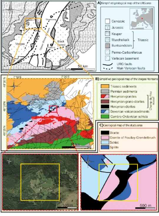
The survey area is located in the Northern Vosges Mountains (Figure 1A), where different units derived from the Hercynian orogeny are outcropping. These units have been widely studied as they are considered to be analogues of the Upper Rhine Graben (URG) basement, where they are the targets of several deep drilling projects for geothermal resource prospecting (Gérard et al., 2006; Vidal and Genter, 2018).

The Northern Vosges basement rocks are composed of different lithotectonic domains stacked together during the Hercynian orogeny between 360 and 300 Ma (Skrzypek et al., 2014). The area of interest is located at the interface between two of these main domains. The Saxothunringian domain is composed of a Devonian basin with a volcano-sedimentary succession metamorphosed under Barrovian conditions (Lardeaux et al., 2014; Skrzypek et al., 2014). The sedimentary rocks are schists and graywackes (light blue, Figure 1B-C), and the volcanics are basalts (blue, Figure 1B-C) that were thermally metamorphosed by the adjacent granite (pink, Figure 1B-C). The granite is part of the Champ-du-Feu domain, a magmatic massif emplaced during the late orogenic extension during the Visean Age. Diorite plutons with varied facies are located along the contact between the granite and the Devonian basin, as in the study area (black, Figure 1B). Since the emplacement of the units and during later tectonic stages namely the Permo-Triassic extension, the opening of the North Atlantic Ocean during the Mesozoic Era and finally the opening of the West European rift in response to the Alpine collision, a complex fault network developed (Bailleux, 2012, p35-40). Many of these

structures reactivate the Hercynian structures. Four sets of orientations are distinguished in the Northern Vosges: the main N-S and NW-SE-oriented faults and ENE-WSW to E-W and

NE-SW-oriented faults (Bertrand et al., 2018).The faults mapped in the field are along the NE-SW contact between the granite and the volcanic sediments and also along the NW-SE contact between the volcanic and sedimentary parts of the Devonian basin (Figure 1B-C).

In addition to the complex geological context, the survey is located around a hamlet, therefore, anthropogenic objects, such as houses, pipelines and various buried ferrous objects, are present. In addition, the hamlet is surrounded by a forest, and only 20% of the area can be accessed on foot for magnetic profiling.

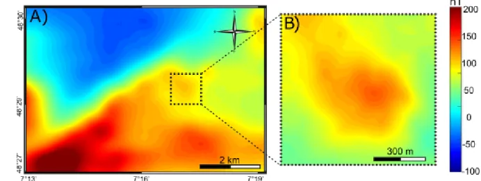
Previous aeromagnetic survey

An heliborne magnetic survey was carried out in 2015 in the Northern Vosges

Mountains. The survey was completed by Geophysics GPR International Inc. using a

Geometrics G-822A caesium magnetometer (Figure 2). The heliborne data were acquired

with a 400 m line spacing at a height of 300 m (AGL). The overall survey shows a good

correlation with the regional-scale lithotectonic domains and structures, and it also provides

new clues about the local fault network, particularly at the Northern Vosges/Upper Rhine

Graben interface (Bertrand et al., submitted). However, the second-order fault network

recognized in the field is only partly observed in the airborne survey. At the Devonian

basin/Champ-du-Feu massif boundary, a main NE-SW lineament was interpreted as a deep

fault hidden at the surface by the diorites. In the area of interest, the magnetic anomaly

linked to this fault is disturbed by a NW-SE lineament that could be the expression of a

second-order NW-SE fault even though it has not been mapped in the field (Figures 1-2).

MAGNETIC DATA ACQUISITION AND PROCESSING

The ground magnetic survey is carried out using backpack equipment manufactured by IPGS (Gavazzi et al., 2016). It allows the simultaneous acquisition of up to eight magnetic profiles spaced at 0.5 m at a height of approximately 0.8 m AGL. Using a head-mounted display, the operator sees the planned profiles he has to follow in real time. Navigation is performed using differential GNSS receivers. The sampling rate of the magnetic data is 25 samples per second. The maximum survey rate is approximately 0.5 ha per hour (Table 1).

The UAV airborne magnetic surveys uses a Matrice 210 RTK quadcopter designed by Da Jiang Innovation (DJI). It has a mean endurance of half an hour using TB55 polymer batteries. Figure 3A shows the UAV equipped with the magnetometer and its electronic device (Figure 3B). This equipment was designed by IPGS and uses a Bartington Instruments Mag-03MC three-axis sensor (Figure 3C) with an overall weight of 484 g and a measurement noise of 6 to 10 pTrms/√Hz. The fluxgate is installed at the tip of a 42 cm long rigid composite pipe in front of the UAV. This distance is a compromise between a longer distance that reduces the electromagnetic noise of the drone and a shorter distance that improves its manoeuvrability. The sampling rate is 25 samples per second. The mean speed along the profiles is approximately 7 m/s, and the mean survey rate is 45 ha per hour at 30 m AGL (Table 1).

Scalar calibration of the sensor and compensation for the UAS

Fluxgate magnetometers are relative sensors, they need to be calibrated. The first step of data processing is related to the calibration of the three components of the magnetometer, because the measurements are dependent on the attitude of the sensor. Calibration is a well-known procedure (Olsen et al., 2003) that involves the computation of nine sensor errors: three for non-orthogonality angles ( ), three for offsets ( ), and three sensitivities ( ). The mathematical solution is found using two assumptions: first, the intensity of the magnetic field is constant in the area where the magnetometer moves in all directions and secondly, the difference between the measured and actual intensities of the magnetic field is only due to the magnetometer errors. The vector magnetic field ⃗ is obtained from the magnetometer output according to (Munschy et al., 2007; Bronner et al., 2013)

[ ] [

√

] [ ] [ ] [ ] ( 1)

The problem is nonlinear for the nine parameters, so, to estimate the parameters, the linearized least-square approach is used (Olsen et al. 2003) and consists in minimizing the χ²-misfit

∑ (

|

⃗ |

)

Where is the intensity of the Earth’s magnetic field in the area where the sensor rotates in all directions and is the data error.

The second step of data processing is related to the compensation of the UAV magnetic effect. Munschy et al. (2007) showed that scalar calibration is the same as magnetic compensation. The UAV magnetic effect is a combination of three sources: the permanent and induced magnetizations and the eddy-current. Using the compensation equations, the permanent magnetization of the UAV corresponds to the offset errors, and the induced magnetization corresponds to non-orthogonality and sensitivity errors (Munschy et al., 2007; Bronner et al., 2013). The eddy currents produce high-frequency electromagnetic noise, which is filtered by the magnetometer and electronic device.

Figure 4 shows the results of the calibration and compensation of the magnetometer for the terrestrial magnetic survey and on board the UAV. In both cases, to obtain the nine errors, the magnetometer’s rotational attitude has to be varied has much as possible in an area where the magnetic field is constant. For the UAV calibration procedure, the drone is in-station at an altitude of about 50 m and the pilot varies the rotational attitude of the drone. It is easy to vary the yaw by 360°. For the roll and pitch, the procedure is more restricted because rotary-wing UAVs are designed to fly with small pitch and roll. The maximum pitch and roll angles obtained during calibration are -50° to -50°. The variations of the magnetometer components during calibration are displayed in Figure 4D1-2. For the terrestrial magnetic survey, the calibration process led to a reduction in the intensity of the magnetic field’s standard deviation from 74.5 to 0.9 nT, and for the UAV, it decreased from 57.1 to 4.6 nT using the same sensor. These results and the corresponding histograms (Figure 4) show that (1) the magnetic effect of the terrestrial equipment is slightly

stronger than that of the UAV; (2) the standard deviation after calibration for the UAV is larger (4.6 compared to 0.9 nT), which is likely due to the local variation in the intensity of the magnetic field in the area of calibration; and (3) the UAV’s histogram is more spread out with a standard deviation of 4.6 nT, but the shape of histogram is similar to a Gaussian distribution.

Survey protocol and data processing

For the ground and airborne surveys, the ratios of sensor height to line spacing range between 0.75 and 1.6 (Table 1) following the recommended specifications for contour mapping of total field magnetic data (Reid, 1980). For airborne surveys, the tie line spacing also follows standards, corresponding to ratios of 1 to 10 for the in-line to tie line spacing.

Three UAV surveys were flown at average flight heights of 1.2, 30 and 100 m AGL. The main goal of the survey at 1.2 m AGL is a comparison with the ground survey results. This comparison covers a small area of 1700 m² (Figure 5). The UAV was flown manually at a mean speed of 1.8 m/s, and the terrestrial equipment was moved at a mean speed of 1 m/s. For the 30 and 100 m AGL surveys, 4 and 2 flights, respectively, of approximately 15 min were necessary in automatic pilot mode at a mean velocity of approximately 8 m/s. These flights cover areas of 47 ha for the 30 m AGL survey and 86 ha for the 100 m AGL survey. The data production in ha/h is highly variable, ranging from 0.5 ha/h for the ground survey to 45 ha/h and 165 ha/h for the UAV surveys at 30 and 100 m AGL, respectively.

For each survey, a magnetic anomaly map is obtained following the standards (e.g.,

calibration/compensation, temporal variation and regional magnetic field corrections, levelling, and grid computation).

RESULTS

Comparison of magnetic data acquired by the UAV and the ground survey

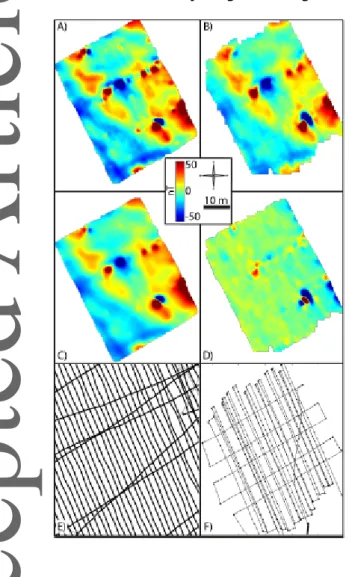
The ground survey has a mean height of 0.80 m AGL, while the UAV survey has a height of 1.20 m AGL. This difference is due to the flight limit of the UAV, particularly the limits of its ultrasonic sensor. Figure 5 shows the magnetic anomaly maps obtained during the ground survey (Figure 5A) and with the UAV (Figure 5B). The maps are similar for both long and short wavelength magnetic anomalies. Minor local differences are observed. For a quantitative comparison, the ground magnetic map is upward-continued (Blakely, 1996) to a height of 1.20 m AGL (Figure 5C), and the differences with the UAV magnetic map (Figure 5D) show that almost all of the magnetic anomalies are the same except for a few with short wavelengths and high amplitudes. These

differences are mainly due to navigation errors, and there is no argument to consider that one of the magnetic maps is better than the other.

Comparison with upward continuation

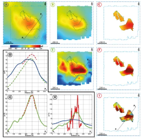
Figure 6 shows a comparison of the three surveys at 100, 30 and 1 m. As expected, the surveys at different altitudes show very different amplitudes and wavelengths. In addition, the clear east-west magnetic lineation observed on the 1 m AGL magnetic map, with an amplitude of

approximately 500 nT (Figure 6I), is smoothed on the 30 m AGL magnetic map (approximately 200 nT, Figure 6E). The 100 m AGL magnetic map mainly shows a circular shape with an amplitude of

approximately 90 nT (Figure 6A). This circular shape is not easily observable on the airborne aeromagnetic map at 300 m AGL (Figure 2), where its amplitude is approximately 20 nT.

The coherency between the three surveys can be studied by upward continuation of the maps. The 1 m AGL (Figure 6I) map is upward continued to 30 (Figure 6F) and 100 m (Figure 6C). For the upward-continuation to 30 m (Figure 6G, red dotted line), the shape of positive part of the anomaly is similar to the data acquired at 30 m. However, for the upward continued map to 100 m (Figure 6C), the intensity and the location is not the same as the acquired data (Figure 6A). These differences are probably due to the fact that the magnetic map at 1 m AGL corresponds to only 20% of the study area, and care must be taken concerning the accuracy of the shape and amplitude of the upward continued maps. The same problem does not occur for the upward continuation of the 30 m AGL magnetic map (Figure 6E) to 100 m AGL (Figure 6B) and the upward continued magnetic map is very similar to the 100 m AGL magnetic map (Figure 6A). For the 30 m AGL upward continued profile (Figure 6D), the difference is likely due to the small area covered by the corresponding survey compared to the survey at 100 m AGL.

Multi-altitude map descriptions

Survey at 100 m AGL

On the 100 m AGL magnetic map, the positive part of a circular anomaly is visible in a large part of the map (Figure 7A). The amplitude of the positive part is 60 nT with a maximum in the centre and an extension outside the mapped area to the NW. This likely corresponds to the NW-SE anomaly observed on the regional map (Figure 2). However, in detail, the geological structure responsible for this anomaly can be divided into two sets of lineaments, NW-SE and NE-SW (Figure 7B). On the geological map, these lineaments can be related to the NW-SE-oriented faults mapped in the metamorphic units that extend into the granite. In addition, the NE-SW-oriented fault at the contact between the granites and the metamorphic units is possibly marked by the left-lateral shift of the magnetic anomaly in the NW part of the map. There is no apparent correlation between the outcropping diorite bodies and the magnetic anomaly map. The origin of these magnetic anomalies is probably due to deep sources.

Survey at 30 m AGL

On the 30 m AGL survey, the horizontal extent of the positive part of the anomaly at 100 m AGL is highly reduced and is divided into 3 anomalies (Figure 7C). The positive maximum is

approximately 150 nT, and it is also located at the centre of the map along a sharp E-W edge. One NW-SE-oriented fault and the NE-SW-oriented faults identified in the 100 m survey can also be identified in the more diffuse part of the anomaly (Figure 7D). However, this part is divided by NNW-ESE to NNE-SSW lineaments that separate local negative and positive areas. Therefore, it appears that this map shows a superposition of the magnetic anomalies due to the deeper structure mapped on the 100 m AGL survey, which is more “diffuse” and highlights regional orientations, and a sharp E-W structures that is likely shallower. This shallower structure does not correspond to a geological feature mapped in the field.

Survey at 1 m AGL

The 1 m AGL survey covers only a small part of the northwestern area (Figure 7E-F). In the northern part, the intensity of the magnetic anomaly progressively increases from south to north of

about 150 nT, but no clear structures are mapped because of the small size of the survey area. Two observations can be made about the sharp anomaly in the centre of the survey area: 1) the clear E-W orientation on the 30 m survey is divided in NE-W-SE to N-S and E-E-W lineaments, and 2) the anomaly is divided in two subparts with positive maxima between 300 and 400 nT that follow the same E-W trend.

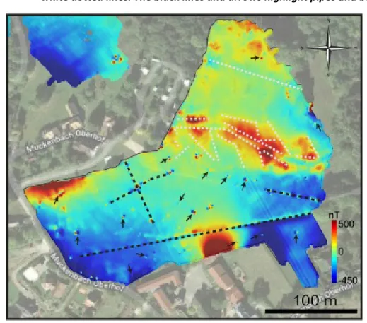
Anthropic structures are also observable on this survey (Figure 8). A main pipe crosscuts the southern area in an ENE-WSW direction with a peak-to-peak RTP anomaly amplitude of 1000 nT, and three others with minor extents and amplitudes are identified (black dotted lines, Figure 8). Small dipolar magnetic anomalies are also scattered in the area and likely correspond to metal objects buried close to surface (black arrows, Figure 8). All of these high-frequency anthropic magnetic anomalies almost completely disappear on the 30 m AGL magnetic map. Therefore, the advantage of magnetic mapping higher above the ground is the strong attenuation of anthropic magnetic signals from shallow sources.

Synthesis for geological interpretation

Because the 100 m survey correlates well with the NW-SE anomaly from the regional airborne survey, it allows a more detailed interpretation of the fault network associated with the anomalies. It is at a more local scale and is compartmentalized by NW-SE and ENE-WSW second-order

structures that correspond to the geological outcrop data as well as the NE-SW fault between the granite and the metamorphic unit. At 30 m AGL, a new step of compartmentalization with roughly N-S faults can be identified. These structural features with structural blocks at different scales and with different fault orientations correspond to recent observations at the regional scale but also at the local scale in the Northern Vosges basement (Bertrand et al., 2018). These features have also been identified in the structure of the URG and in others rifting environments (Le Garzic et al., 2011), and they are documented well here by the UAV surveys.

The local faults are currently not mapped in the field because of the poor outcrop conditions (e.g., forest, hamlet and farming fields). However, the fault orientations are consistent with regional faults and fractures, namely, the N-S orientation documented by recent studies (Elsass et al., 2008; Bertrand et al., 2018). The sharp E-W anomaly is consistent in the 30 m and 0.8 m surveys but also has not been observed in the field. However, it could be a dyke crosscutting the granite, as is documented in other parts of the magmatic massif (Elsass et al., 2008). Finally, we also note the clear absence of a magnetic signal linked to the diorite intrusion. This is likely due to a weak

difference in their magnetic susceptibilities and/or the absence of a clear structural contact between the diorites and the granite. It is also possible that these diorites have a complex 3D extent at shallow depths because the cartographic limit of the unit is not consistent with that of a simple magmatic pluton.

CONCLUSIONS

Fluxgate magnetic measurements with a rotary-wing UAV are possible and fill the gap between ground magnetic mapping and aeromagnetism. This new technique of magnetic mapping is also

more efficient than ground magnetic surveying and allows mapping of areas inaccessible on the ground.

Scalar calibration corrects both the sensor-related measurement errors and the magnetic effects of the UAV. This method allows the sensor to be mounted directly on the UAV, avoiding the

complexities associated with towing the magnetic sensor. In addition, by using light fluxgate magnetometers directly installed on the UAV, any size UAV can be used.

The four magnetic maps presented (300, 100, 30 and 1 m AGL) show magnetic anomalies with very different amplitudes, shapes, wavelengths and orientations. Depending on the height above the ground of the survey platform, the magnetic anomalies emphasise magnetic sources with different depths. Specifically, the structural interpretation (Figure 7) shows a wealth of structural orientation data, which increase in detail with decreasing height. However, the high-resolution data close to the ground do not highlight the regional orientations of the structures.

ACKNOWLEDGMENTS

The authors wish to thank Fonroche Géothermie, who provided access to the aeromagnetic data. IPGS (Institut de Physique du Globe de Strasbourg) is acknowledged for partial funding of the UAV. CONFLICTS OF INTEREST

LIST OF FIGURES

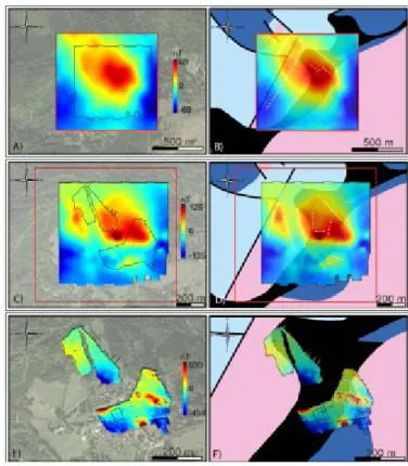
Figure 1: A) Regional geological map of the Upper Rhine Graben (URG) (modified after Bossennec et al. (2018)). B) Simplified geological map of the Vosges Mountains (modified after Bertrand et al. (2018)). C) Geological map of the survey area (right) and satellite image (left). The yellow square corresponds to the dashed black square in Figure 2.

Figure 2: A) Heliborne magnetic anomaly map at 300 m above ground level. The dashed black square indicates the survey site. B) UAV magnetic anomaly map at 100 m above the ground.

Figure 3: A) UAV Matrice 210 RTK (DJI) equipped with the electronic device (B) and the Bartington MAG03-MC fluxgate magnetometer (C). The overall weight of the magnetic equipment is 484 g.

Figure 4: Calibration and compensation results. A1-2) The two curves correspond to the non-corrected (blue line) and non-corrected (red line) intensities of the magnetic field. B1-2)

Histograms of the intensity of the magnetic field after calibration. C1-2) Calibration parameters and their errors. D1-2 the three components of the magnetometer during calibration. 1 corresponds to the terrestrial magnetic survey results, and 2 corresponds to the UAV results.

Figure 5: A) Ground magnetic anomaly map at 0.8 m AGL. B) UAV magnetic anomaly map at 1.20 m AGL. C) Upward continuation of the ground magnetic anomaly map to 1.20 m AGL. D) Difference between two magnetic anomaly maps B and C. See location in Figure 7F. E) Track chart of the ground magnetic map. F) Track chart of the UAV magnetic map.

Figure 6: A) UAV magnetic anomaly map at 100 m AGL. B) Upward continued magnetic anomaly map at 30 m AGL to 100 m. C) Upward continued magnetic anomaly map at 1 m AGL to 100 m. D) Magnetic anomaly profiles at 100 m. Continuous lines correspond to the magnetic profiles extracted from the magnetic maps, and dotted lines correspond to the profiles extracted from the upward continued maps. E) UAV magnetic anomaly map at 30 m AGL. F) Upward continued magnetic anomaly map at 1 m AGL to 30 m. G) Magnetic anomaly profiles at 30 m. Continuous lines correspond to the magnetic profiles extracted from the magnetic maps, and dotted lines correspond to the profiles extracted from the upward continued maps. H) Magnetic anomaly profiles P1-P2 from the 1 m AGL (red line), 30 m AGL (green line) and 100 m AGL (blue line) maps. I) Ground magnetic anomaly map at 1 m AGL.

Figure 7: A) Magnetic anomaly maps after reduction to the pole (I=64.2° and D=1.6°) at 100 m AGL superimposed on a satellite image. B) Magnetic anomaly maps after reduction to the pole at 100 m AGL superimposed on the geological map. C) Magnetic anomaly maps after reduction to the pole at 30 m AGL superimposed on a satellite image. D) Magnetic anomaly maps after reduction to the pole at 30 m AGL superimposed on the geological map. E) Magnetic anomaly maps after reduction to the pole at 1 m AGL superimposed on a satellite image. F) Magnetic anomaly maps after reduction to the pole at 1 m AGL

superimposed on the geological map. The structural interpretations are shown on the right by white dotted lines. The black rectangle represents the magnetic map shown in Figure 5.

Figure 8: Magnetic anomaly map after reduction to the pole of the ground survey in the south superimposed on a satellite image. The structural interpretation is shown by the white dotted lines. The black lines and arrows highlight pipes and buried metal.

Table 1 Statistics of the surveys.

Ground

UAV

HELICOPTER

Number

of sensors

4

1

1

Height

(m)

0.80

1.2

30

100

300

Profile

spacing

(m)

0.5

1-Feb

30

100

400

Tie line

spacing

(m)

~20

~6

~150

200

4000

Mean

speed

(m/s)

0.9

1.8

7.5

8

42

Coverage

(ha/h)

0.5

0.75

45

165

2900

REFERENCES

Bailleux, P., 2012. Multidisciplininary approach to understand the localization of geothermal anomalies in the Upper Rhine Graben regional to local scale. Phd. thesis, University of Neuchâtel, 35-40.

Bertrand, L., Jusseaume, J., Géraud, Y., Diraison, M., Damy, P.-C., Navelot, V., Haffen, S., 2018. Structural heritage, reactivation and distribution of fault and fracture network in a rifting context: Case study of the western shoulder of the Upper Rhine Graben. Journal of Structural Geology. 108, 243–255. https://doi.org/10.1016/j.jsg.2017.09.006

Bertrand, ., a azzi, ., ercier de pina , ., iraison, ., raud, ., unsch , ., su mitted. On the use of aeromagnetism for geological interpretation part II: geological interpretation on outcropping basement rocks as analogs for geothermal prospects. Submitted to Journal of Geophysical Research, Solid Earth.

Blakely, R.J., 1996. Potential Theory in Gravity and Magnetic Applications. Cambridge University Press, p 313-319.

Bossennec, C., Géraud, Y., Moretti, I., Mattioni, L., Stemmelen, D., 2018. Pore network properties of sandstones in a fault damage zone. Journal of Structural Geology 110, 24–44.

https://doi.org/10.1016/j.jsg.2018.02.003

Bronner, A., Munschy, M., Sauter, D., Carlut, J., Searle, R., Maineult, A., 2013. Deep-tow 3C magnetic measurement: Solutions for calibration and interpretation. Geophysics 78, J15–J23.

https://doi.org/10.1190/geo2012-0214.1

Caron, R.M., Samson, C., Straznicky, P., Ferguson, S., Sander, L., 2014. Aeromagnetic surveying using a simulated unmanned aircraft system. Geophysical Prospecting 62, 352–363.

https://doi.org/10.1111/1365-2478.12075

Cunningham, M., Samson, C., Wood, A., Cook, I., 2018. Aeromagnetic Surveying with a Rotary-Wing Unmanned Aircraft System: A Case Study from a Zinc Deposit in Nash Creek, New Brunswick, Canada. Pure and Applied Geophysics 175, 3145–3158. https://doi.org/10.1007/s00024-017-1736-2

Davis, K., Li, Y., Nabighian, M., 2010. Automatic detection of UXO magnetic anomalies using

extended Euler deconvolution. Geophysics 75, G13–G20. https://doi.org/10.1190/1.3375235 Eck, C., Imbach, B., 2012. Aerial magnetic sensing with an UAV helicopter. ISPRS - International

Archives of Photogrammetry, Remote Sensing and Spatial Information Sciences XXXVIII-1/C22, 81–85. https://doi.org/10.5194/isprsarchives-XXXVIII-1-C22-81-2011

Elsass, P., von Eller, J.P., Stussi, J.M., 2008. Géologie du massif du Champ du Feu et de ses abords. Eléments de notice pour la feuille géologique 307 Sélestat (No. BRGM/RP-56088-FR). Everett, M.E., 2013. Near-Surface Applied Geophysics. Cambridge University Press.

https://doi.org/10.1017/CBO9781139088435, 34-51.

Fassbinder, J. W. E., 2016, Magnetometry for Archaeology: Encyclopedia of Geoarchaeology, Encyclopedia of Earth Sciences Series, 499–514.

Funaki, M., Higashino, S.-I., Sakanaka, S., Iwata, N., Nakamura, N., Hirasawa, N., Obara, N., Kuwabara, M., 2014. Small unmanned aerial vehicles for aeromagnetic surveys and their flights in the South Shetland Islands, Antarctica. Polar Science. 8, 342–356.

https://doi.org/10.1016/j.polar.2014.07.001

Gavazzi, B., Le Maire, P., Munschy, M., Dechamp, A., 2016. Fluxgate vector magnetometers: A multisensor device for ground, UAV, and airborne magnetic surveys. The Leading Edge 35, 795–797. https://doi.org/10.1190/tle35090795.1

Gee, J.S., Cande, S., Kent, D.V., Partner, R., Heckman, K., 2008. Mapping geomagnetic field variations with unmanned airborne vehicles. EOS 89, 177–180.

Gérard, A., Genter, A., Kohl, T., Lutz, P., Rose, P., Rummel, F., 2006. The deep EGS (Enhanced Geothermal System) project at Soultz-sous-Forêts (Alsace, France). Geothermics 35, 473– 483. https://doi.org/10.1016/j.geothermics.2006.12.001

Hinze, W., von Frese, R.R.B., Saad, A.H., 2013. Gravity and magnetic exploration. Cambridge University Press, 215-233.

ardeaux, . ., Schulmann, K., Faure, ., anoušek, V., exa, O., Skrz pek, E., Edel, . ., Štípská, P., 2014. The Moldanubian Zone in the French Massif Central, Vosges/Schwarzwald and Bohemian Massif revisited: differences and similarities. Geological Society London Special Publications. 405, 7–44. https://doi.org/10.1144/SP405.14

e arzic, E., de ’Hamaide, T., iraison, ., raud, ., Sausse, ., de Urreiztieta, ., Hau ille, ., Champanhet, J.-M., 2011. Scaling and geometric properties of extensional fracture systems in the proterozoic basement of Yemen. Tectonic interpretation and fluid flow implications. Journal of Structural Geology 33, 519–536. https://doi.org/10.1016/j.jsg.2011.01.012 Leach, B.W., 1980. Aeromagnetic compensation as a linear regression problem, in: Information

Linkage Between Applied Mathematics and Industry. Elsevier, pp. 139–161. https://doi.org/10.1016/B978-0-12-628750-9.50017-6

Leliak, P., 1961. Identification and Evaluation of Magnetic-Field Sources of Magnetic Airborne Detector Equipped Aircraft. IRE Transactions on Aerospace Navigational Electronics ANE-8, 95–105. https://doi.org/10.1109/TANE3.1961.4201799

Macharet, D., Perez-Imaz, H., Rezeck, P., Potje, G., Benyosef, L., Wiermann, A., Freitas, G., Garcia, L., Campos, M., Macharet, D.G., Perez-Imaz, H.I.A., Rezeck, P.A.F., Potje, G.A., Benyosef, L.C.C., Wiermann, A., Freitas, G.M., Garcia, L.G.U., Campos, M.F.M., 2016. Autonomous

Aeromagnetic Surveys Using a Fluxgate Magnetometer. Sensors 16, 2169. https://doi.org/10.3390/s16122169

Malehmir, A., Dynesius, L., Paulusson, K., Paulusson, A., Johansson, H., Bastani, M., Wedmark, M., Marsden, P., 2017. The potential of rotary-wing UAV-based magnetic surveys for mineral exploration: A case study from central Sweden. The Leading Edge 36, 552–557.

https://doi.org/10.1190/tle36070552.1

Munschy, M., Boulanger, D., Ulrich, P., Bouiflane, M., 2007. Magnetic mapping for the detection and characterization of UXO: Use of multi-sensor fluxgate 3-axis magnetometers and methods of interpretation. Journal of Applied Geophysics 61, 168–183.

https://doi.org/10.1016/j.jappgeo.2006.06.004

Nabighian, M.N., Grauch, V.J.S., Hansen, R.O., LaFehr, T.R., Li, Y., Peirce, J.W., Peirce, J. D. Phillips, and M. E. Ruder, 2005. The historical development of the magnetic method in exploration. Geophysics 70. https://doi.org/10.1190/1.2133785

Olsen, N., Tøffner-Clausen, L., Sabaka, T.J., Brauer, P., Merayo, J.M., Jørgensen, J.L., Léger, J.M., Nielsen, O.V., Primdahl, F., Risbo, T., 2003. Calibration of the Ørsted vector magnetometer. Earth Planets Space 55, 11–18.

Pan, Q., Liu, D.-J., Guo, Z.-Y., Fang, H.-F., Feng, M.-Q., 2016. Magnetic anomaly inversion using magnetic dipole reconstruction based on the pipeline section segmentation method. Journal of Geophysics and Engineering 13, 242–258. https://doi.org/10.1088/1742-2132/13/3/242 Parshin, A.V., Morozov, V.A., Blinov, A.V., Kosterev, A.N., Budyak, A.E., 2018. Low-altitude

geophysical magnetic prospecting based on multirotor UAV as a promising replacement for traditional ground survey. Geo-Spatial Information Science 21, 67–74.

https://doi.org/10.1080/10095020.2017.1420508

Parvar, K., Braun, A., Layton-Matthews, D., Burns, M., 2017. UAV magnetometry for chromite exploration in the Samail ophiolite sequence, Oman. Journal of Unmanned Vehicle Systems https://doi.org/10.1139/juvs-2017-0015

Primdahl, F., 1979. The fluxgate magnetometer. Journal of Physics E: Scientific Instruments. 12, 241–253. https://doi.org/10.1088/0022-3735/12/4/001

Reid, A.B., 1980. Aeromagnetic survey design. Geophysics 45, 973–976.

Ripka, P., 2003. Advances in fluxgate sensors. Sensors and Actuators A : Physical 106, 8–14. https://doi.org/10.1016/S0924-4247(03)00094-3

Roelof, V., McKay, M., Anderson, M., Johnson, R., Selfridge, B., Bennett, J., 2007. Feasibility Study for an Autonomous UAV -Magnetometer System. Idaho National Laboratory (INL).

https://doi.org/10.2172/923485

Salem, A., Ravat, D., Gamey, T.J., Ushijima, K., 2002. Analytic signal approach and its applicability in environmental magnetic investigations. Journal of Applied Geophysics 49, 231–244. Samson, C., Straznicky, P., Laliberté, J., Caron, R., Ferguson, S., Archer, R., 2010. Designing and

building an unmanned aircraft system for aeromagnetic surveying, in: SEG Technical Program Expanded Abstracts 2010. Society of Exploration Geophysicists, 1167–1171. https://doi.org/10.1190/1.3513051

Sherrod, B.L., Blakely, R., Lasher, J.P., Lamb, A., Mahan, S.A., Foit, F.F., Barnett, E.A., 2016. Active faulting on the Wallula fault zone within the Olympic-Wallowa lineament, Washington State, USA. Geological Society of America Bulletin 128, 1636–1659.

https://doi.org/10.1130/B31359.1

Skrzypek, E., Schulmann, K., Tabaud, A.-S., Edel, J.-B., 2014. Palaeozoic evolution of the Variscan Vosges Mountains. Geological Society London Special Publications 405, 44–75.

Stoll, J.B., 2013. Unmanned aircraft systems for rapid near surface geophysical measurements. International Archives of the Photogrammetry, Remote Sensing and Spatial Information Sciences, XL-1/W2

Tuck, L., C. Samson, C. Polowick, et J. Laliberté, 2019. Real-Time Compensation of Magnetic Data Acquired by a Single-Rotor Unmanned Aircraft System. Geophysical Prospecting.

https://doi.org/10.1111/1365-2478.12800.

Vidal, J., Genter, A., 2018. Overview of naturally permeable fractured reservoirs in the central and southern Upper Rhine Graben: Insights from geothermal wells. Geothermics 74, 57–73. https://doi.org/10.1016/j.geothermics.2018.02.003

Walter, C.A., Braun, A., Fotopoulos, G., 2018. Impact of 3-D Attitude Variations of a UAV Magnetometry System on Magnetic Data Quality. Geophysical Prospecting. https://doi.org/10.1111/1365-2478.12727

Walter, C.A., Braun, A., Fotopoulos, G., 2020. High-Resolution Unmanned Aerial Vehicle Aeromagnetic Surveys for Mineral Exploration Targets. Geophysical Prospecting, 68, 334-349. https://doi.org/10.1111/1365-2478.12914

Wells, M., 2008. Attenuating magnetic interference in a UAV system (Text). Master of Applied Science, Carleton University.

Wood, A., Cook, I., Doyle, B., Cunningham, M., Samson, C., 2016. Experimental aeromagnetic survey using an unmanned air system. The Leading Edge 35, 270–273.