HAL Id: hal-00316243
https://hal.archives-ouvertes.fr/hal-00316243
Submitted on 1 Jan 1997
HAL is a multi-disciplinary open access archive for the deposit and dissemination of sci-entific research documents, whether they are pub-lished or not. The documents may come from teaching and research institutions in France or abroad, or from public or private research centers.
L’archive ouverte pluridisciplinaire HAL, est destinée au dépôt et à la diffusion de documents scientifiques de niveau recherche, publiés ou non, émanant des établissements d’enseignement et de recherche français ou étrangers, des laboratoires publics ou privés.
Initial observations of fine plasma structures at the flank
magnetopause with the complex plasma analyzer SCA-1
onboard the Interball Tail Probe
O. L. Vaisberg, L. A. Avanov, V. N. Smirnov, James L. Burch, A. W. Leibov,
E. B. Ivanova, J. H. Waite Jr., A. A. Klimashev, B. I. Khazanov, I. I.
Cherkashin, et al.
To cite this version:
O. L. Vaisberg, L. A. Avanov, V. N. Smirnov, James L. Burch, A. W. Leibov, et al.. Initial observations of fine plasma structures at the flank magnetopause with the complex plasma analyzer SCA-1 onboard the Interball Tail Probe. Annales Geophysicae, European Geosciences Union, 1997, 15 (5), pp.570-586. �hal-00316243�
Initial observations of fine plasma structures at the flank
magnetopause with the complex plasma analyzer SCA-1
onboard the Interball Tail Probe
O. L. Vaisberg1, L. A. Avanov1, V. N. Smirnov1, J. L. Burch3, A. W. Leibov1, E. B. Ivanova1, J. H. Waite, Jr.3, A. A. Klimashev2, B. I. Khazanov2, I. I. Cherkashin2, M. V. Iovlev2, A.Yu. Safronov2, A. I. Kozhukhovsky1, C. Gurgiolo3, V. H. Lichtenstein4
1Space Research Institute, Russian Academy of Sciences, 84/32 Profsoyuznaya str., 117810 Moscow, Russia 2
State Research Institute of Scientific Instrumentation, 6 Raspletina str., 123060 Moscow, Russia
3
Southwest Research Institute, 6220 Culebra Road, P.O. Drawer 28510, San Antonio, Texas 78228-0510, USA
4Kurchatov Institute, Moscow, Russia
Received: 20 May 1996 / Revised: 1 October 1996 / Accepted: 15 October 1996
Abstract. The fast plasma analyzer EU-1 of the SCA-1
complex plasma spectrometer is installed onboard the Interball Tail Probe (Interball-1). It provides fast three-dimensional measurements of the ion distribution func-tion on the low-spin-rate Prognoz satellite (about 2min). The EU-1 ion spectrometer with virtual aperture con-sists of two detectors with 16 E/Q narrow-angle analyz-ers and electrostatic scannanalyz-ers. This configuration allows one to measure the ion distribution function in three dimensions (over 15 energy steps in 50 eV/Q–5.0 keV/Q energy range in 64 directions) in 7.5 s, which makes it independent of the slow rotation speed of the satellite. A description of the instrument and its capabilities is given. We present here the preliminary results of measurements of ions for two cases of the dawn low-and mid-latitude magnetopause crossings. The proper-ties of observed ion structures and their tentative explanation are presented. The 12 September 1995 pass at low latitude at about 90° solar-zenith angle on the dawn side of the magnetosphere is considered in more detail. Dispersive ions are seen at the edge of the magnetopause and at the edges of subsequently ob-served plasma structures. Changes in ion velocity distribution in plasma structures observed after the first magnetopause crossing suggest that what resembles multiple magnetopause crossings may be plasma blobs penetrating the magnetosphere. Observed variations of plasma parameters near magnetopause structures sug-gest nonstationary reconnection as the most probable mechanism for observed structures.
1 Introduction
The complex plasma spectrometer SCA-1 is intended to measure characteristics of magnetospheric ions on the Tail Probe of the Interball Project. The main features of SCA-1 are its fast 3D capability provided by an elect-rostatic scanner, relatively large coverage of velocity
space (960 bins in the main measurement mode), and an absence of averaging in velocity space. We give a short description of the instrument (for a more detailed description see Vaisberg et al. 1995) and present the first results of its observations of magnetopause plasma structures at the dawn of the Earth’s magnetosphere.
The boundary layer as a transition between the magnetosheath and magnetosphere proper was identi-fied by Hones et al. (1972) and Akasofu et al. (1973). The high-latitude portion of the boundary layer (plasma mantle) was first observed by Rosenbauer et al. (1975) and studied in more detail by Gosling et al. (1984) and Siscoe et al. (1994). Magnetosheath plasma was found to enter directly into the tail lobe (Gosling et al., 1984; Mozer et al., 1994), in agreement with the slow-mode MHD expansion fan model of the plasma mantle (Siscoe and Sanchez, 1987). Entry regions commonly lie on the flanks of the tail with north-south asymmetry (Gosling
et al., 1985), like those predicted by Cowley (1981b) as a
result of dayside merging with IMF.
The low-latitude boundary layer (LLBL) on the closed magnetic field lines on the dayside was observed by Eastman et al. (1976), Paschmann et al. (1976), Crooker (1977), Haerendel et al. (1978), and Eastman and Hones (1979). Le et al. (1996) demonstrated two types of LLBL for northward IMF: heated magneto-sheath plasma in the outer boundary layer and a mixture of magnetosheath and magnetospheric plasma in the inner boundary layer. Boundary layers with heated magnetosheath plasma are more likely to be observed near the subsolar region. The boundary layer with only the mixture-type plasma is mainly observed near the dawn and dusk flanks. This is consistent with previous observations of LLBL in dawn and dusk flanks using three-dimensional data sets by Eastman et al. (1985).
The entry of solar-wind plasma into the magneto-sphere (driving magnetospheric process) can possibly be accounted for, at least in part, by the Kelvin-Helmholtz (K-H) instability (Axford and Hines, 1961).
Several local and nonlocal mechanisms producing boundary layers have been discussed. Dungey proposed
reconnection as a solar wind-magnetosphere coupling mechanism; he also mentioned the possibility of cusp reconnection for northward IMF (Dungey, 1963). Ev-idence for magnetic reconnection at the subsolar mag-netopause for southward IMF was obtained by Russell and Elphic (1978), Sonnerup and Ledley (1979), Son-nerup et al. (1981), and Gosling et al. (1982). A non-local entry mechanism in the cusp region via turbulent convection process accompanied by magnetic reconnec-tion has been suggested by Haerendel et al. (1978). Cusp reconnection has been proposed by Cowley (1981a) and Song and Russell (1992) as a possible mechanism for plasma entry and the LLBL formation for northward IMF.
Signatures associated with reconnection include acceleration of the magnetosheath plasma to speeds greater than those in the adjacent magnetosheath (Sonnerup, 1981; Paschmann et al., 1979, 1986, 1990; Phan et al., 1994), reversals of flow direction near the dayside magnetopause (Gosling et al., 1990a), and separation of electron edge earthward of ion edge during accelerated flow events (Vaisberg et al., 1980; Gosling et al., 1990b). Direct observational evidence for reconnection of the open field lines of the tail lobe with the IMF at high latitudes when the local magne-tosheath field and lobe field are nearly antiparallel was given by Omel’tchenko et al., (1983) and Gosling et al., (1991).
Dungey (1955) pointed out the possibility that the K-H instability could develop as a result of the solar-wind interaction with the magnetosphere. Satellite observations of multiple quasi-periodic structures near the magnetopause were interpreted in terms of the K-H instability developing at the inner edge of the boundary layer (Sckopke et al., 1981), surface waves on the magnetosphere (Lepping and Burlaga, 1979; Couzens
et al., 1985), vortex structures on the far tail boundary
layer (Hones et al., 1981), and the plasma inclusions in the boundary layer that suggest transport across the magnetopause (Larson and Parks, 1992).
Miura (1984, 1987, 1992) studied the K-H (MHD) instability as a drive diffusive process for LLBL, evidence for its role in viscous transport, and conse-quences of the K-H instability for the solar wind-magnetosphere interaction. The hybrid simulations show the presence of small-scale structures that separate from the boundary (Thomas and Winske, 1991, 1993). The relative importance of the K-H instability for the solar-wind entry is thought to be minimal (~10% effect) compared to reconnection (Baumjohan and Paschmann, 1987).
The local entry mechanism via diffusion was consid-ered by Eastman et al. (1976) and Eastman and Hones (1979). Gary and Eastman (1979) proposed lower hybrid drift (kinetic) instability as a drive diffusive process for LLBL. However, the transition from magnetosheath to the boundary layer is often thin (less than an ion’s gyroradius) and the plasma within the boundary layer is uniform, suggesting that diffusion is not important (Sckopke et al., 1981; Song et al., 1990; Le et al., 1994). Another local entry mechanism, impulsive penetration,
was proposed by Lemaire and Roth (1978), Lemaire (1985) and Ross (1992).
Quasi-periodic pulses of magnetosheath-like plasma on magnetic field lines near the dawn magnetopause observed on ISEE 1/2 were interpreted as evidence for the strong diffusion of magnetosheath plasma across the magnetopause, and the K-H instability at the inner edge of the LLBL (Sckopke et al., 1981), as evidence for magnetic merging and the formation of twisted flux ropes of interconnected magnetosheath and magneto-spheric field lines (Paschmann et al., 1982), and as quasi-periodic magnetopause motions and observation of draped northward magnetosheath magnetic field lines in the plasma depletion layer (Sibeck et al., 1990). K-H instability can accelerate the reconnection rate (LaBelle-Hammer et al., 1988; Liu and Hu, 1988). Reconnection and the K-H instability may be interconnected; obser-vations suggest that accelerated flow associated with reconnection can excite K-H instability (Saunders, 1989).
Three-dimensional observations of ions provide a useful tool for detailed analysis of different MHD and kinetic processes in magnetospheric plasmas, giving better determination of flow parameters and details of the ion distribution functions. A three-dimensional plasma analyzer SCA-1 having a relatively fast duty cycle (less than 10 s) and moderate angular and energy resolution is installed on the Interball-1/Tail Probe satellite. It provides ion measurements much faster than the period of the satellite’s rotation (120 s), enabling one to study plasma evolution at magnetospheric boundaries and relevant processes. We present here a description of the instrument, show examples of data, and give preliminary explanation of observed plasma structures.
2 Instrumentation
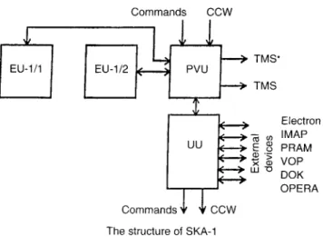
A three-dimensional multichannel scanning analyzer EU-1 is part of the complex plasma spectrometer SCA-1. It is serviced by an onboard computer PVU and controlling device UU-1. The structure of SCA-1 is shown in Fig. 1.
The SCA-1 was designed and built in Russia under contract between the IKI and SNIIP Institute, Moscow. The Southwest Research Institute contributed signifi-cantly to the calibration of the instrument.
2.1 EU-1
The ion E/Q spectrometer EU-1 has full three-dimen-sional capabilities. Its two identical sensor heads EU-1/1 and EU-1/2 both have nearly hemispheric fields of view. A schematic view of the EU-1 analyzer is shown in Fig. 2a. Each sensor head consists of a toroidal electro-static analyzer (ESA) for measurements of ions entering the wide circular aperture, according to their energy/ charge ratio. The selected energy is determined by the bipolar voltages on the electrodes of the electrostatic analyzer.
A microchannel plate electron multiplier (MCP) of OlenT-M type, followed by an eight-sectored anode, is installed at the narrow circular exit of the electrostatic analyzer, and allows one to measure eight E/Q ion spectra simultaneously. In order to minimize the cross-talk between analyzers resulting from the properties of the toroidal analyzer and from the spread of electron beam in the MCP stack, several diaphragms are installed in front of the MCP stack and between the MCPs. The FWHM of each individual analyzer is 2°. The fields of view of all analyzers are nearly coaligned (being evenly distributed in azimuth along the cone of 2°opening angle).
In order to provide measurements over a nearly 2p field of view, an electrostatic scanner is installed in front of the toroidal electrostatic analyzer. It allows one to redirect the apertures of all eight individual narrow-angle electrostatic analyzers simultaneously, so they are look-ing in eight evenly spaced directions along the cone with an opening angle controlled by the electrostatic scanner. In this way measurements in three dimensions can be performed much faster than the satellite’s spin period.
The electrostatic scanner in front of the analyzer’s input window consists of two electrodes. The inner electrode is a hemisphere and the outer electrode, being under the potential of the housing, is a part of cone covered from the input side with a conductive grid. Depending on the (negative) voltage applied to the inner hemispheric electrode of the scanner, only those ions enter the entrance aperture of the electrostatic analyzer that arrive at a certain angle (with respect to the instrument’s field-of-view axis). This scanner provides a maximum unobscured field of view about 70° from the main axis of the detector. Deflection of the angular aperture of analyzers by the electrostatic scanner leads to some increase in the widths of angular diagrams of individual analyzers.
As the hemispheric electrode is biased by a negative potential, it may be a source of electrons under UV-radiation of the Sun. Therefore, we decided to shield the inner electrode of the scanner from sunlight with a buffer that allows the ions to enter the instrument. Ray tracing within the chosen geometry of the scanner was performed, and the shades’ shape and location were chosen for selected deflection angles of ions. The sunshade baffle in front of the analyzer was tested with an ion beam and proved to be reasonably good, both in terms of the amount of ion transmission and of shading of scanner’s hemispherical electrode.
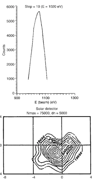
The calibration of the EU-1 detectors was performed in IKI and SwRI vacuum test chambers. Examples of energy and angular diagrams are shown in Fig. 3.
The energy range of the instrument is 50 eV/Q–5.0 keV/Q, scanned in logarithmically spaced energy steps. The FWHM of the energy passband is ~10%. Both 15-energy-step scans and 30-15-energy-step scans are used in different modes of the instrument. Four polar angles are provided by the potentials applied to the scanner: non deflected scan (designated 2°direction), and three deflec-tions from the axis of symmetry of detector: 17°, 40°, and 65°. Characteristics of the instrument are given in Table 1.
Fig. 1. The structure of SCA-1. It consists of two 2p sensor heads
EU-1/1 and EU-1/2, an onboard computer PVU, and controlling device UU-1
Fig. 2. a A schematic view of EU-1 analyzer. Sensor head consists of a
toroidal electrostatic analyzer, channel electron multiplier MCP, followed by eight-sectored anode, electrostatic scanner consisting of central spherical electrode and grid-covered conic electrode, and sunshade baffle (collimator). b Sketch showing the viewing directions of two sensor heads of an instrument installed on rotating spacecraft. Sun direction is indicated by arrow
One of the analyzers, EU-1/1, is installed on the satellite so that its field-of-view axis is pointed along the satellite axis directed toward the Sun, while the other detector, EU-1/2, is oriented in the opposite, antisolar direction. Figure 2b shows a diagram of the instrument’s position on the spacecraft and the relation of the spin
axis and the solar direction to the field of view of the instrument.
The EU-1 instrument works automatically under PVU control. PVU controls modes of measurements through changing voltages of the analyzer and scanner, controls pulse counters, and receives the results of measurements. PVU also performs onboard calculations of plasma parameters in real time.
Two basic modes of EU-1 operation are possible through digital control of the analyzer and scanner voltages by PVU:
1. Consecutive measurements of energy spectra over 30 or 15 (even or odd ones) energy steps in the energy range 0.05–5.0 keV/Q in four or two (even or odd ones) different angular directions: 2°, 17°, 40°, and 65°relative to the symmetry axes of solar and antiso-lar analyzers. The duration of each energy step is 1/ 1024 of the spacecraft rotation period (as determined by the spin clock signal).
2. In parallel in eight angular azimuthal channels of each analyzer at a fixed energy step and a fixed deflection angle.
The satellite spin period T is divided into 1024 intervals t T/1024 that equals to 117 ms for nominal
T 120 s satellite spin. The MCP’s pulse accumulation
time is 90 ms, with the rest being used for transition to the next energy step. The pulse counters are locked at that time. After the measurements at maximum energy are made, there is a voltage setting cycle during which the analyzer voltage goes down to minimum. This time-interval equals 2t. Sequential measurements of energy spectra at four angles define a complete cycle of measurement. This cycle provides nearly a full scan of the three-dimensional ion distribution function. Eight complete cycles may be made per satellite spin. The number of cycles may be increased if the scanned energy intervals are reduced.
Accumulated counts in 16 azimuthal directions are stored by 2-byte words. The typical data flow speed from EU-1 working in the fast mode is 256 bytes/s.
2.2 Modes of operation
Each instrument of Interball is limited in the informa-tion that can be recorded in onboard memory, as well as by time of real-time transmission. Therefore, the full information capacity of SCA-1 can be used only along a limited part of the satellite trajectory, and the rest of the orbit is covered by slow modes.
Upon switching on and during initialization two tasks are performed: diagnostics, D, and background measurements, B. There are seven measurement modes: three slow ones M1, M2, and M3, two accelerated modes U1 and U2, and two fast modes NP1 and NP2, called direct data transmission modes. During the diagnostic task the microprocessor, RAM, ROM, timer, pulse counters, communication ports, amplifiers-dis-criminations, and low- and high-voltage power supplies are tested.
Fig. 3. Examples of energy (above) and angular (below) diagrams of
EU-1
Table 1. Characteristics of EU-1/SCA-1
Parameter
Energy range, E/Q, keV 0.05–5.00 Number of energy steps 15 or 30,
depending on mode (Ei+1–EI) / Ei+1, % 17
Energy resolution, FWFM, % 10
Azimuthal directions 8, separated by 45° Polar directions 2°, 17°, 40°, 65°,
115°, 140°, 163°, 178° Angular resolution, FWHM 2°
Geometric factor, cm2sr 5×10)4
Temporal resolution 7.5 s (9-s average due to buffer memory overload)
During the second task voltages at the electrostatic generator are set to zero, and background values of all 16 sectors of CEMs are recorded separately for each sector and for 16 uniformly spaced phases of the satellite spin (the data are averaged over intervals of 64t). These values are stored in PVU-RAM and are used in subsequent calculations.
The mode NP1 (first real-time mode) provides the fastest measurements of the three-dimensional distribu-tion funcdistribu-tion. The scanning of the energy spectrum is performed simultaneously by 16 analyzers (eight with a sunward-looking detector and eight with an antisun-ward-looking detector) over 15 energy steps and for four deflection angles h 2°, 17°, 40°, and 65°sequentially. Each energy scan is performed in about 1.8 s, thus a total cycle of measurements in 64 angular directions over the sphere takes 7.5 s. In this mode the space/time resolution increases by a factor of two compared to the one in the case of full scanning.
The mode NP2 (second real-time mode) is used for measurements of fast variations of the ion distribution function. The angle and energy value E are set at fixed values by a control command word (CCW), and the count rates of all detectors, sampling 16 phase-space bins, are measured with a frequency of 8 Hz. This provides simultaneous measurements in two ring sec-tions of velocity space.
In the mode M1 (first slow mode) the following parameters are calculated, using the assumption that all ions are protons:
n: ion number density;
Vx,, Vy, Vz: three components of the velocity vector (in
the satellite coordinate system);
Ti: ion temperature;
Qx, Qy, Qz: three components of the energy flux vector;
A, B: parameters of distribution function, strong
chang-es of which are used for the initialization of fast (alert) mode.
In this mode the background values, recorded in the
B mode, are subtracted from the numbers of counted
pulses: The RAM of the PVU stores the following constants that are necessary for these calculations: S the value of sensitivity of the analyzers for given angle; values of energies E/Q, and trigonometric func-tions for allh and u angles (in the spacecraft coordinate system). Parameters are calculated at the end of the measurement cycle.
The parameters obtained in the previous cycle are stored in RAM. In the M1 mode there are eight measurement cycles per one satellite spin. The compres-sion rate in this mode compared to the NP modes equals 128.
The mode M2 (second slow mode) is analogous to M1, but the data compression rate is higher, i.e., 4 measurement cycles are averaged (over the half-spin of the satellite) for calculations of n, V, Tiand Q.
Mode M3 consists of different submodes. A three-dimensional distribution function measured within one satellite spin is recorded alternatively with plasma parameters calculated in a manner similar to the M1
or M2 mode acquired over several spins. Depending on the contents of the relevant CCW, a full energy/angular distribution is measured either once (at the beginning of the spin) or twice (at the beginning and in the middle of the spin). Furthermore, the CCW sets the number of spins (from 1 to 128) during which only calculated parameters are recorded before the next three-dimen-sional distribution. The resulting data compression rate varies between 2 and 400. Mode M3 can be set for any number of satellite spins, from 2 to 16512, i.e., from 4 min up to 123 day’s duration.
In the mode U1 (first accelerated mode) the three-dimensional ion distribution is measured during a time 32t by a reduced manner. In submode U1a 15 odd energy steps in one angular sector alternate with 15 even steps in the next angular sector. In the mode U1b the measurements are made over the same energy-step sequence for every angular sector.
The direction and energy step during which the corrected counting rate is maximum are determined and recorded in the telemetry frame along with following sections of ion distribution: energy spectrum in the direction of recorded maximum and h-u spherical section at the energy step of recorded maximum.
The mode U2 (second accelerated mode) is analogous to the second fast mode, in which fast plasma fluctua-tions with a frequency 8 Hz are performed in two ring sections of velocity space with predetermined h and E values. Measurements in this mode can be carried out only during 10 s.
The modes are selected either by telecommands, or as a result of EU-1 data processing by PVU, or by alert signals from other instruments (IMAP, ELECTRON, PRAM, OPERA, DOK, VDP). Turning on the accel-erated mode from a slow mode occurs in two cases: if one of the instruments gives an unconditional alert signal or three or more instruments give conditional alert signals. When the alert signal is worked out by SCA-1, it is also transmitted to other instruments, which can also use this signal to turn to accelerated mode. The accelerated mode of SCA-1 is turned on for about five spins of the satellite.
The data from EU-1 and the results of primary data processing are transmitted to telemetry in frames of a standard size of 128 byte including 8-bytes header.
Due to the fact that the memory dump speed of information system SSNI of Interball-1 exceeds the real-time mode speed, most of the fast data of EU-1 are prerecorded in the memory of the SSNI information system.
2.3 PVU device
The specialized onboard micro-controller PVU includes a microprocessor, RAM, ROM, and timer. It also includes two buffers that receive from RAM the results of measurement in the format required by the telemetry system SSNI.
The capacity of the ROM is 8 Kbytes; the RAM’s 16 Kbytes. Cold redundancy is used to increase the PVU’s
reliability. In addition, there are certain special hard-ware and softhard-ware means of protection against possible failures.
The PVU controls the operation modes of the EU-1, performs processing of the data and controls the data flow. EU-1 and PVU form a subcomplex which is able to operate independently. The complex is organized so that the EU-1 transmits the accumulated data into the PVU periodically after certain time-intervals and per-forms other data exchange operations. In addition the microprocessor provides data processing (calculation, analysis of the acquired data, etc.). Due to considerable volume of such operations an autonomous calculator was introduced in the PVU structure.
2.4 UU controlling device
A controlling device UU performs the following func-tions in organizing the SCA-1 work:
1. exchanges signals with several scientific instruments on the spacecraft (mentioned already as ‘‘external’’ instruments);
2. received board time code (BTC) from the onboard systems, records it in when measurements are per-formed, and makes this code ready for recording in an output TM frame;
3. receives the signal of the beginning of the satellite’s spin around its axis (spin clock), and works out the time-grid that determines the sequence of the instru-ments functioning;
4. receives CCWs and relay commands (RCs), records them and prepares the needed data to set the mode of operation for PVU.
2.5 Status of SCA-1 complex
The SCA-1 complex was activated on 14 August, 1995, after a designated outgassing period. The three-dimen-sional ion spectrometer EU-1 has a very low back-ground, and good sensitivity. The measurement pro-gram provides high-resolution data in both NP-1 and NP-2 modes from interesting regions, including the bow shock, magnetosheath, plasma sheet, and tail lobes. There were periods when the fast mode was triggered by the alert signal of another instrument.
Present functioning of SSNI results in an overflow of information in the instrument buffer that leads to stops in the measurement cycle for about 3.2 s every 12.8 s. Therefore, in the NP-1 mode 12–14 complete three-dimensional ion distribution functions are obtained every 120-s spin period of satellite instead of the planned number 16.
2.6 Data analysis
Software for SCA-1 data analysis includes routines for data structure reconstruction, dynamic spectra and velocity distribution function plotting, and calculation of moments of the distribution function. Main flow
parameters were calculated usually as moments of distribution, obtained by the extension of measured phase-space density to the respective volume of phase space with allowance for relative sensitivities of 16 detectors. The latter were determined from laboratory calibration data and tested against omnidirectional ion flux in the plasma sheet. Estimated present uncertainty of velocity calculations is several km/s for high-density plasma, and about 30 km/s for low-density plasma. The estimated error in number-density calculations is now within a factor of 2. A Maxwellian fit was used for tests of parameters calculated as moments of measured distribution. Calculations of flow parameters were made in the supposition that all ions are protons. This is justified in most of the cases when plasma of solar-wind origin is measured, as protons constitute about 95% of the solar-wind flow.
2.7 Comparison with other instruments
The SWE plasma instrument on the WIND spacecraft (Ogilvie et al., 1995) has a VEIS detector with slightly smaller coverage of the velocity space (576 for VEIS compared to 960 for SCA-1), but a wider energy range, 7 eV–24.8 keV. VEIS also has faster mode (6-s temporal resolution), but it is not clear how frequently and for how long this fast mode is implemented. VEIS has six detectors and uses fast spacecraft rotation to measure three-dimensional ion (and electron) distribution.
Another plasma and energetic particle instrument on WIND (Lin et al., 1995) has ion analyzers PESA-L and PESA-H which have 40 detectors with an angular resolution from 5.6° to 22.5° within a circular field of view, and which sweep in the energy range 3 eV–30 keV 32 or 64 times per 3-s spin. However, ion-velocity distribution is transmitted only once per minute or in the short-burst mode. Most of the time only moments of distribution are transmitted.
The Low-Energy Particle Experiment onboard the GEOTAIL satellite (Mukai et al., 1994) is with ions in the energy range from several eV/q to 43 keV/q. Seven MCPs located at the exit of the quadrispheric electro-static analyzer are used to cover seven narrow angular sectors within the meridional angular diagram of the instrument. One 3-s spin period of the satellite is divided into 16 azimuthal sectors. The energy range is divided into 32 energy intervals. Complete three-dimensional ion distribution over 3584 velocity space bins is measured over 12 s (four spacecraft rotations).
The CPI instrument on the GEOTAIL spacecraft has a hot-plasma electrostatic analyzer CPI-HS for hot electrons and ions (Frank et al., 1994). It uses nine discrete channel electron multipliers to measure ions in nine relatively wide angular sectors situated approxi-mately along the meridional plane of the satellite. Azimuthal scanning is provided by spacecraft rotation. A frequent mode for measuring the three-dimensional velocity distribution of ions consists of a 1728-sample determination of ions in 18 s over 32 energy passbands in the range 22 eV–48 keV. This is done by the division
of the spacecraft rotation period (3 s) into eight azimuthal sectors.
SCA-1 has a narrower energy range than most of the mentioned instruments; it has, however, a sufficiently detailed sampling of the velocity space (960 bins) and quite a fast speed (within 10 s in the fast mode). These qualities are fully used by initiating continuous fast mode of measurements of ion-velocity distributions for several hours around interesting regions of geospace.
3 Observations
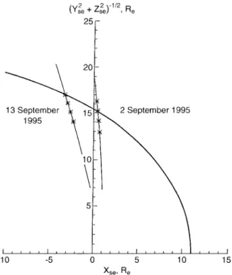
We will concentrate on initial results of observations near the dawn magnetopause. We discuss here two magnetopause crossings, observed in NP1 mode, that show plasma behavior near the boundary. The first one occurred on 2 September 1995 at about 0145 UT at GSM coordinates: X 0.5 Re, Y)14.3 Re, and Z 2.6 Re
(Fig. 4). The second set of magnetopause-associated events was observed on 13 September 1995 starting at about 0900 UT in the GSM coordinates location:
X 0:4 Re, Y )13.8 Re, and Z 8.4 Re, (Fig. 4).
3.1 2 September 1995 case
Figure 5 shows the counting-rate spectra of EU-1 with measurements performed in NP1 prerecorded mode during the magnetopause crossing on 12 September 1995. During this crossing the satellite was moving approximately along the-Y-axis. In order to compress
the time-scale the counts of all eight analyzers of sunward-facing sensor head (four upper panels) are summed, as well as the counts of all eight analyzers of antisunward sensor head (four lower panels). This gives eight dynamic spectra measured along cones 2°, 17°, 40°, 65°, 115°, 140°, 163°, and 178°from the nearly sunward axis of the satellite’s rotation. The color scale on the right shows the counts per accumulation time 0.09 s. The 2-min periodicity seen on some dynamic spectra is due to small nutation of the instrument axis.
The magnetosheath spectrum with a maximum at about 300 eV and highly anisotropic distribution is easily seen in the four upper panels before 0145 UT. At that time the magnetosheath spectrum changes to a plasma-sheet-type spectrum that is much more isotropic and is seen in all eight panels as increased counting rate in the upper part of the energy range (the counting-rate spectrum of the electrostatic analyzer emphasizes higher energies as its energy-geometric factor is proportional to energy squared). Magnetosheath particles are also seen in the magnetosheath starting at 0126 UT. Additional detail seen at magnetopause is a narrow beam in the four lower panels. As we will show, this beam has an energy dispersion so that lower energies are observed first, close to the magnetopause, and the energy of the ions in the end of the beam is higher than that of the magnetosheath spectrum. Several plasma features observed during the subsequent time interval resemble successive crossings of the magnetopause. It is interesting to note some ion flux observed from the antisunward hemisphere at energies of magnetosheath ions and higher.
Figure 6 shows two counting-rate spectra of EU-1 for the same magnetopause crossing on 2 September 1995 along with main flow parameters: number density, N, total flow velocity, V0, and ion temperature, Ti. The two
counting-rate diagrams at the top are the sums of all eight azimuthally spaced analyzers, one from the sun-ward-facing sensor head during measurements at the deflection angle from the nearly sunward axis of satellite’s rotation h 17°, and another from the antisunward-facing sensor head during measurements at deflection angle h 140°. Thus these two panels represent measurements along two cones. The color scale on the right shows ‘‘integrated’’ over these cones summed by eight azimuthal sector counts per accumu-lation time 0.09 s.
Many plasma features are observed during the time-interval after the first magnetopause crossing. Most of them within the time interval 0145–0235 UT resemble successive crossings of the magnetopause. However, maximum counting rate and calculated number density fall as the satellite moves deeper into the magnetosphere. The successive reappearance of magnetosheath-type plasma resembles bursts. These bursts have nearly the same energy spectrum as that of the magnetosheath if we look at the upper panel (sunward hemisphere). On the lower panel (antisunward hemisphere) these bursts are wider in time-scale, looking as envelopes of bursts seen in the sunward hemisphere. One may notice energy dispersion in the antisunward hemisphere (lower panel) resembling the beam at the magnetopause crossing.
Fig. 4. Interball-1 orbits in cylindric coordinate system with X-axis
oriented towards the Sun. Parts of orbits for which data are presented in the paper are indicated by 1-h separated tick marks. Average magnetopause location is shown for reference
Fig. 5. Counting rate spectra of EU -1 with me asure ments performe d in NP-1 p rerecorde d m ode during magnetopause crossing on 12 Septembe r 1995. At thi s ti me the sate llite was moving approximately along-Y -axis. In order to compress the time-scale the counts o f a ll eigh t a nalyz ers of sunward-fac ing sensor h ead (fo ur upper panels ) a re summe d, as well as the counts o f a ll eight analyzers of anti sunward sensor h ea d (fo ur lower pan els ). This gives eight dynamic spectra measure d a long cones 2 ° ,1 7 ° ,4 0 ° ,6 5 ° ,1 1 5 ° ,1 4 0 ° , 163 ° , a nd 178 ° from nearly sunward axis o f satellite’s rota tion. Color scale on the right show s the counts p er accumulation time 0.09 s; 2-min periodicity seen on some dynamic spectra is due to small nutation of instrument axis Fig. 6. The two counting-ra te diagrams on the top are the sums of all eight azimuthally spac ed analyzers, one from sunward-facing sens o r h ea d w it h m easurements at deflec tion a ngle from nearly-sunward a xi s o f sate llite ’s rotation h 17 ° , a nd anot her one from antisunward-facing sensor h ea d w ith measurem ents at deflec ti o n a ngl e h 14 0 ° . T hus these two panels repr esent measurements along two cones. The color sc ale o n the right shows ‘‘integrat ed’’ o ver thes e cones counts p er acc u mulation time 0.09 s. The lowe r three panels are calculated flow parame ters (mome n ts of dis tribution function), calc u lated in the supposition that a ll ions ar e p rotons: number d ensity, N , total flow velocity, Vo , a nd io n tem perature, Ti
These properties are more clearly seen for bursts located in the sunward hemisphere at 0147, 0219, and 0233 UT. It is easy to see that where flux has a maximum in solar hemisphere, there is a minimum flux in the antisunward hemisphere.
After 0240 UT bursts look even more diffuse. Flux is lower, structure is less distinct, and the maximum in the sunward hemisphere is less pronounced. Still, the burst as seen in the sunward hemisphere is narrower than in the antisunward hemisphere. Maximum flux and the lower-energy cut-off and average energy in the plasma burst are progressively displaced to higher energies. Plasma-sheet-type particles are slightly depressed within the burst (see burst at 0249 UT). Part of these features are also seen in some earlier bursts (0214, 0229 UT).
Another feature of transition from magnetosheath to magnetosphere is the appearance of magnetospheric ions in the magnetosheath in the layer adjacent to the magnetopause. As one may see, ions in the energy range above 1 keV appeared as a separate part of the distribution in the counts of antisunward-looking ana-lyzers at about 0126 UT, and continued to be registered through the magnetopause (these ions are not distin-guishable in the counts of sunward-looking detectors due to their higher counting rates in this energy range). The leakage of magnetospheric ions through the mag-netopause is considered an indication of reconnection (see, for example, Phan et al., 1994).
The peculiarities of the magnetopause crossing and trend in the properties of plasma clouds along the spacecraft trajectory is seen also in flow parameters (three lower panels of Fig. 6). Number density in mag-netosheath remained nearly constant for about 45-min time-interval. Two dropouts (at ~0127 and ~0139 UT) are associated with velocity jumps (second panel from below). Periodic fluctuations in number density with a period of 120 s are artifacts associated with the rotation of the instrument axis around the axis of the satellite’s rotation and relatively large azimuthal spacing between analyzers, 45°, leading to fluctuations in counting rates (however, this has little influence on calculated flow velocity and temperature). The velocity of magneto-sheath plasma slightly increased during the time interval shown, and exhibits several jumps, ranging from about 30 to 70 km/s. The first velocity jump, at~0113 UT, is accompanied by the leakage of magnetospheric parti-cles, and the largest jump, at about 0126 UT, marks the start of a region of permanent magnetospheric-ion leakage to the magnetosheath. The velocity increase of about 30 km/s is also seen just before the magnetopause crossing. Ion temperature, approximately constant be-fore 0126 UT, increases in the time interval, when
magnetospheric ions are added to the magnetosheath flow, and this increase is apparently associated with this admixture. However, the temperature drops somewhat before the magnetopause crossing. Slight temperature increases are associated with velocity bursts, except the burst at~0113 UT, which marks the magnetosheath-ion-leakage region, in front of which temperature increased by a factor of two. It is not clear at this stage of analysis whether these temperature increases are associated with plasma heating or with a drop in magnetosheath-plasma number density accompanied by the appearance of magnetospheric ions in the same plasma volume.
Flow parameters show how plasma bursts change with increasing distance from the magnetopause. Num-ber density in plasma bursts drops as the satellite moves deeper into the magnetosphere, although maximum number density reaches its magnetosheath value in the first half of magnetospheric region shown. Maximum velocity values observed in the plasma bursts in the magnetosphere initially reach higher than average values in the magnetosheath (time-interval 0248–0209 UT), then sometimes reach the magnetosheath value (time-interval 0218–0232 UT), but average flow velocity in bursts continually decreases with increasing distance from the magnetopause. Velocity correlates quite well with num-ber density. Ion temperature in plasma bursts in the magnetosphere shows systematic increase from its mag-netosheath value (about 70 eV) to the temperature value of magnetospheric ions (about 2 keV), and is approxi-mately inversely correlated with ion number density.
Figure 7 shows how the ion-velocity distribution function changes at the magnetopause and in the first plasma burst. Each small panel shows angular distribu-tion on the fixed energy step of ion counting rate obtained by smoothing measurements over 64 angular bins (eight bins in azimuthu, shown horizontally from 0°to 360°, by eight bins in elevationh, from 0°– nearly sunward direction – at the top to 180° – nearly antisunward direction – on the bottom). Each vertical row is a complete three-dimensional measurement frame at 15 logarithmically spaced energies (indicated on the left) from 60 eV at the bottom to 4.26 keV at the top. It is taken, on average, over less than 10 s. Time corres-ponding to the beginning of each 6th measurement frame is shown at the bottom of the diagram. For ease of reference each frame is numbered at the top. The color scale codes counting rate in the manner shown in Fig. 6, slightly modified to emphasize low counts. Red horizontal bands in the 10th frame are glitches in the measurement sequence not yet removed. The time-interval shown is slightly over 5 min, i.e., about 2.5 satellite rotations.
Fig. 7. Ion velocity distribution function changes at magnetopause
and in the first plasma burst. Each small panel is angular distribution of the ion counting rate on the fixed energy step obtained by smoothing over measurements in 64 angular bins (8 bins in azimuth u, shown horizontally from 0°to 360°, by 8 bins in elevationh, from 0°, nearly sunward direction, at the top to 180°, nearly antisunward direction, on the bottom). Each vertical row is a complete three-dimensional measurement frame at 15 logarithmically spaced energies
(indicated on the left). Time corresponding to the beginning the each 6th measurement frame is shown on the bottom of the diagram. Each frame is numbered on the top for reference. Red horizontal bands on 11th frame are glitches
Fig. 8. Ion velocity distribution function changes in the fifth plasma
burst. The format of the figure is the same as for Fig. 7; see text for details
Magnetosheath distribution functions close to the magnetopause (frames 0 to 6) show varying density that steeply decreases in frames 5 and 6, still keeping the identity of convected plasma flow. Contrary to that, frames 7 to 9 show ion beams initially, in frame 7, coming from the sunward hemisphere (energy range 0.18 – 1.20 keV), and then from antisunward hemisphere (energy ranges 0.28–1.64 keV in frame 8 and 0.46–2.26 keV in frame 9). The slight trace of the returning beam is still seen by the energy 2.28 keV in frame 10.
Magnetospheric plasma is seen in three upper ener-gies throughout the diagram. It is nearly omnidirection-al in magnetosphere proper (frames 11–15 and 29–30), but is slightly depressed and convected in the magneto-sphere and plasma burst.
Energy and angular distribution, as well as counting rate, in the plasma burst are very much like magneto-sheath ones. However, distributions at two edges of burst are quite different. Frames 15 and 16 show beams, coming at about 90°to the satellite axis, at elevation and azimuth quite different to the plasma-flow direction in the plasma burst. Frames 27–29 show the beam quite similar to what was seen at the magnetopause crossing. In frames 26 and 27 the beam is coming from an approximately solar direction. In frames 28 and 29 the beam is coming from the antisunward hemisphere. Again, as at the magnetopause, energy dispersion or low-energy cut-off is seen: ion flux is observed at 0.26–1.64 keV in frame 28, and at 0.63–1.64 keV in frame 29.
Figure 8 shows changes in ion-velocity distribution function at the fifth plasma burst. The structure of the figure is the same as Fig. 7. The observed burst has a complicated structure. In the beginning (frames 0 to 2) the angular and energy distributions are quite similar to those observed in the magnetosheath (differences seen in the diagram are due to different azimuthal phasing from Fig. 7). All subsequent frames show distributions con-sisting of ion beams coming mostly from the solar direction (e.g., frames 6, 11, and 16), from the antisolar direction (e.g. frames 23 and 25–28), or from two directions (frames 10, 13, 22, and 24). Again, at the edge of the burst we see the same structure of the rotating beam: one coming from the solar hemisphere in frame 24, and subsequently another coming from the antisolar hemisphere with the energy dispersion (frames 25–28). High-energy magnetospheric ions are almost excluded from the plasma burst except for the convected compo-nent in frames 0–4 and 17–20. The dispersive rotating beam in frames 25–28 marks the edge of the burst exterior to which omnidirectional high-energy magnetospheric ions are observed (frames 27–30).
Figure 9 compares plasma and magnetic field pa-rameters for the magnetopause crossing on 2 September 1995 and gives some derived parameters for the same time interval. Vx(Fig. 9e) shows that, within the
uncer-tainty of velocity calculation for low-density plasma, all plasma bursts observed after about 0210 UT are non-convected (except for front edge of 5th cloud). Jumps of transverse velocity Vt at the edges of bursts are due to beams.
The sampling rate of FM-3 magnetometer for the 2 September pass was one vector in 32 s that complicates detailed comparison with temporal variations of plasma. Magnetic filed (Fig. 9e) in the magnetosphere is about 25 nT and is directed approximately along the Z-axis. Average Bz in the magnetosheath is negative and
facilitates reconnection. All velocity bursts in the mag-netosheath after 0127 UT are accompanied by changes in Bzsign, and the magnetic-field magnitude within these
events approaches magnetospheric value. This is an indication of reconnection processes.
Figure 9f compares plasma ram pressure, Pd qV2,
ion thermal pressure, NkTiand magnetic-field pressure,
Pm B
2
/8p. Remembering uncertainty in ion number-density calculations, we can check what plasma features are still convecting, and which ones cannot propagate across the magnetic field, by comparing ram pressure with magnetic pressure. This comparison confirms that many bursts, especially those observed after 0210 UT, are nonconvecting or slowly convecting plasma fea-tures.
Ion thermal pressure remains approximately constant along the satellite’s pass. Slight depressions are seen in the hot magnetospheric-ion domains, apparently due to limitations of the instrument. It underestimates the density and, probably , the temperature of hot ions due to a limited upper energy range and to a low-energy-geometric factor at low energies.
3.2 13 September 1995 case
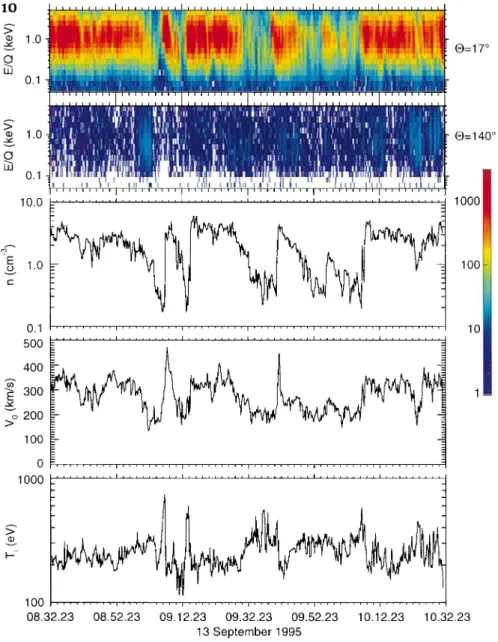
Figure 10 shows the counting-rate spectra of two elevation cones of EU-1 during the satellite pass in the vicinity of the magnetopause on 13 September 1995 along with computed flow parameters, similar in format to that of Fig. 6. During this crossing the satellite was at GSM coordinates X 0.4 Re, Y )13.8 Re, and
Z 8.4 Re (Fig. 4). Measurements start and end in
the magnetosheath, and there are several potential magnetopause crossings and plasma bursts, most pro-nounced at 0906 and 0939 UT.
The average magnetic field in the magnetospheric side was Bx~+ 10 nT, By~+ 15 nT, and Bz~+12 nT. So
the satellite crossed the magnetopause on the flank above the equator where magnetic field lines are closed and draped. The magnetic field in magnetosheath was very disturbed; Bzwas changing from about +8 to )15
nT in the time interval shown; By and Bz were in the
range from ~ +10 nT to ~ )10 nT and quite variable. Average magnetic-field magnitude in magnetosheath is about 10 nT.
The first tentative magnetopause crossing within the time interval under discussion was at about 0859 UT. It is characterized by the strong decreases in number density and velocity, and by isotropization of ions seen as increased flux from the antisunward hemisphere (second panel from above in Fig. 10) and as a modest temperature increase (lower panel in Fig. 10).
The plasma burst starting at about 0906 UT is characterized by strong increases in temperature,
veloc-ity, and number density. Temperature starts to rise first, and reaches maximum at the velocity front. Velocity starts to rise before the number density jumps, but reaches maximum just after number density rises to a plateau at the magnetosheath value. The maximum temperature is about 750 eV, more than six times the magnetosheath value of about 120 eV. Maximum velocity is 470 km/s, about 140 km/s above the average magnetosheath value of 330 km/s. Velocity drops faster than number density, reaching 190 km/s at the end of the burst, about 140 km/s below the magnetosheath value.
Quite a similar plasma-parameter profile is seen at the plasma burst starting at about 0940 UT. The temperature pulse precedes the velocity pulse. However, the peak of the velocity pulse approximately coincides with the moment when number density reaches mag-netosheath value. Other differences from the event at
0906 UT are a shorter duration of temperature and velocity increases, and a larger number-density increase length.
Number-density jumps from the magnetospheric value to magnetosheath values starting at 0913 and 0940 UT are also accompanied by strong temperature pulses at the boundary, but maximum velocity at the boundary does not increase above average magneto-sheath value. There are small density increases above the average magnetosheath value in both cases. These boundaries may be tentatively identified as outward magnetopause crossings. A smaller density pulse at about 0956 UT resembles the partial magnetopause crossing. All inbound magnetopause crossings and rear ends of plasma bursts are quite smooth. Most noticeable plasma signature of bursts compared to magnetopause crossings are very large excursions of plasma velocity at the front edges of the bursts.
Fig. 9a–f. Comparison of plasma and
magnetic-field parameters and some de-rived parameters for magnetopause crossing on 2 September 1995. a proton number density N; b total velocity Vo, c
Vx(thin curve) and transverse Vt(thick
line) velocity components, d ion
temper-ature, e magnetic field magnitude Bo
(thick line) and Bz(thin line) component
(from FM-3 magnetometer data), f plasma ram pressure, Pd qV2(thin
line), ion thermal pressure, NkTi, (lower
thick line) and magnetic-field pressure, Pm B2/8p (upper thick line)
4 Discussion
Two cases of phenomena at the low-latitude magneto-pause at the flank of the magnetosphere presented here show the variety to transient plasma phenomena at the magnetopause, including velocity bursts in the magne-tosheath, the mixture of the magnetosheath and mag-netospheric plasma and plasma clouds in the magneto-sphere. Two cases have different locations: the 2 September case is almost on the geomagnetic equator, and the satellite enters the magnetospheric region with nearly northward magnetic field populated by plasma-sheet particles. The 13 September case is significantly northward, magnetospheric filed lines are stretched, and, as we can infer from measurements of ions in our energy range, boundary-layer ions are observed on magnetospheric side with no trace of energetic magne-tospheric ions.
The two cases are very much different in terms of magnetosheath plasma and magnetic-field
characteris-tics. Plasma velocity is significantly higher for the 13 September case. The magnetosheath magnetic field is nearly southward and steady for the 2 September case that facilitates reconnection. On 13 September the magnetic field is highly variable.
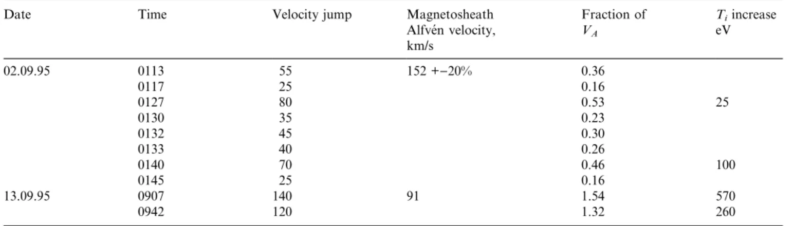
Transients in the 2 September case are seen as velocity bursts in the magnetosheath and as plasma bursts in the magnetosphere (Fig. 6). Table 2 gives the magnitude of velocity jumps observed in the magneto-sheath in comparison with Alfve´n-velocity values in the magnetosheath. Magnitudes of velocity increases are in the range of 10s km/s. Only in two cases of eight velocity bursts does the magnitude reach about 0.5 VA, the
average being about 0.3 VA. Some of the velocity bursts
are accompanied by density decreases. Only a small fraction of the magnetosheath bursts are accompanied by temperature increases. Plasma bursts on the magne-tospheric side of the 2 September pass also show velocity increases above the mean magnetosheath value by about 50 km/s, comparable in magnitude to velocity jumps in
Fig. 10. The counting-rate spectra for two
elevation cones of EU-1 during satellite pass in the vicinity of magnetopause on 13 September 1995 along with computed flow parameters, similar to format of Fig. 6
the magnetosheath (see bursts 1 to 4). However, in these cases noticeable temperature jumps were not observed.
Nearly antiparallel magnetic fields at the magneto-sheath and at magnetospheric sides of the 2 September magnetopause crossing suggest reconnection as a reason for velocity jumps in the magnetosheath and for plasma bursts in magnetosphere. This is supported by the registration of hot magnetospheric ions in the magne-tosheath at the time of the 0113 UT burst and continued leakage of magnetospheric ions after the burst at 0127 UT. Another possible reason for velocity bursts in the magnetosheath and plasma bursts in the magnetosphere observed on 2 September could be the K-H instability.
Whatever the reason of transients in the 2 September case, it is worthwhile to note that the duration of disturbances observed in magnetosheath is nearly equal to the duration of the region of plasma bursts in the magnetosphere. The time-interval where velocity bursts and the leakage of magnetospheric ions are observed continuously (0126–0145 UT), about 19 min, favorably compares to the region on the magnetospheric side, where plasma bursts are strongest (0145–0205 UT), about 20 min. The total time-interval of transients in the magnetosheath from the first velocity burst (0113–0145 UT), about 32 min, can be compared to the time-interval of the observation of moderate bursts still bearing the same signatures of magentosheath plasma (0145–0225 UT), about 40 min. This suggest the same process forming disturbances in the two regions. If we assume that the magnetopause was, on average, in nearly the same location during satellite transition through disturbance regions, we may estimate with the use of spacecraft velocity the width of the strong interaction region to be about 2500 km.
Plasma bursts observed on 13 September (Fig. 10) have been observed while the satellite was on magneto-spheric side, presumably in the boundary layer. Magni-tudes of velocity increases (Table 2) are even above magnetosheath Alfve´n velocity. There were strong temperature increases on the fronts of the bursts, both in magnitude and in comparison with the respective magnetosheath value. Strong temperature increases indicate an energization process, and fast flows are an important indication of reconnection processes
(Son-nerup et al., 1981; Paschmann et al., 1979, 1986, 1990; Phan et al., 1994; Gosling et al., 1990a).
So it appears that bursts observed in the magneto-sheath on 2 September have different characteristics from ones observed on 13 September. Firstly, they constitute different fractions of respective magneto-sheath Alfve´n velocities (Table 2). Another difference between the two cases lies in the temperature increases on the fronts of the bursts, which are much stronger in the 13 September case, both in magnitude and in comparison with respective magnetosheath values.
Plasma bursts observed on the magnetospheric side of the 2 September case show interesting evolution with time, or distance from the magnetopause (Fig. 6). Initially they very much resemble successive magneto-pause crossings (bursts 1 to 3 and part of burst 4). The trend in the properties of plasma bursts along the spacecraft trajectory is seen in the flow parameters. Average number density and transport velocity decrease as the satellite moves deeper into the magnetosphere, and temperature increases. As one can see in the counting-rate spectrograms (two upper panels on Fig. 6), the average energy of ions and low-energy cut-off increase with the distance from the magnetopause, and the relative flux from the antisunward hemisphere increases. It seems reasonable to assume that we are observing the evolution of distinct plasma features as the satellite moves deeper into the magnetosphere.
The difference of beams observed at the front edge of the plasma burst (frames 15 and 16 on Fig. 7) and one at the rear edge of the plasma burst (frames 26–29 on Fig. 7) also support the suggestion that these bursts are not just repetitive crossings of the magnetopause rather than separate plasma blobs (term used by Sckopke et al., 1981) or ‘‘tongues’’ of plasma, possibly similar to those developing in the K-H instability simulation (Thomas and Winske, 1993). Repetitive crossings of the magne-topause should show the same pattern on two sides of the plasma burst, reversed in time; however observations show different patterns on two sides.
The change of properties of plasma bursts along the satellite trajectory is confirmed by the evolution of the ion distribution function (Figs. 7 and 8). Initially (see burst 1, Fig. 7, frames 17–25), ions have a velocity
Table 2. Velocity jumps above magnetosheath value and Alfve´n velocity
Date Time Velocity jump Magnetosheath Alfve´n velocity, km/s Fraction of VA Tiincrease eV 02.09.95 0113 55 152 +)20% 0.36 0117 25 0.16 0127 80 0.53 25 0130 35 0.23 0132 45 0.30 0133 40 0.26 0140 70 0.46 100 0145 25 0.16 13.09.95 0907 140 91 1.54 570 0942 120 1.32 260
distribution similar to that of the magnetosheath (same figure, frames 0–6). Kinetic effects are seen at that time only on the edges of the burst (frames 15–16 and 26–29, Fig. 7). Later in time the ion distribution function changes drastically (burst 5, Fig. 8). Only on the front edge of burst 5 (frames 0–2) does the plasma still resemble the magnetosheath. The main body of plasma in the burst has a quite different velocity distribution, and ion beams constitute the significant portion of it. This trend is seen through the whole succession of plasma bursts.
Ions in the bursts moving up in the energy tend to join the hot magnetospheric plasma population, as seen in the sequence of bursts 5, 6, and 7 (Fig. 6). It suggests that the plasma seen in the bursts may be a source factor for this magnetospheric population.
An interesting feature of the 2 September case is the observed ion beam coming from the antisunward hemisphere both at the first magnetopause crossing and at the rear edge of the plasma clouds. This beam shows energy dispersion being less energetic close to the plasma boundary, and more energetic further out. Typical transition of returning beam from about 300 eV (100-km proton gyroradius in the 25-nT field) to about 800 eV (160-km proton gyroradius in the 25-nT field) takes about 30 s in the spacecraft frame, which translates to a spacecraft velocity relative to the plasma feature of about 2 km/s. The orbital velocity of the spacecraft in the region of plasma-burst observation on 2 September was about 1 Re/h, which gives 1.8 km/s.
This suggests that the transverse velocity of the boundary is small.
The 2 September case shows that the mean energy of ions in the bursts systematically increases with time as the satellite moves deeper into the magnetosphere. This starts from the rear edge of burst 3, and is quite evident in bursts 4–7 (except the dense region in first half of burst 5). Energy per ion increases well above available from convetive and thermal ion motion in adjacent magnetosheath and in bursts 1–3 observed close to magnetopause crossing. It means that the energization mechanism works at the same time as the plasma feature dissipates. The mechanism that provides the increase in the average energy of ions in the plasma feature may probably be identified by detailed analysis of plasma and magnetic field data.
At present it is not clear what the topological properties of observed plasma features, or blobs, are. They may be three-dimensional structures (clouds) or elongated field tubes, a more probable case due to anisotropy introduced by the magnetic field. Further analysis of the plasma velocity distribution and mag-netic field is required before any statement on topology of this features can be made.
Energization of ions in bursts observed farther from magnetopause crossing and observed evolution of dis-tribution function suggest that this plasma may subse-quently integrate to hot magnetospheric population (plasma-sheet-type ions). This is confirmed by very dilute clouds observed after 0300 on 2 September (not
shown). These clouds are barely distinguishable from the hot magnetospheric population.
The penetration of plasma features from the magne-tosheath into the magnetosphere may be a possible source of the plasma-sheet population. Its importance is unclear at this time and requires analysis of statistically significant number of cases.
Kinetic effects at the magnetopause associated with steady reconnection were observed by Fuselier et al. (1995). These results were based on analysis of mass-resolved measurements and showed reflected and trans-mitted populations both for magnetospheric and for magnetosheath plasma. Observations discussed here are another demonstration of kinetic effects at magneto-pause, and may be a useful tool for diagnostics of processes in hot magnetospheric plasmas.
The tentative explanation of some observed effects as associated with nonsteady reconnection awaits more detailed analysis of stress and energy conditions (Cowl-ey, 1995; Sonnerup et al., 1995) and will be the topic for subsequent work.
5 Conclusions
1. The fast three-dimensional plasma spectrometer SCA-1 provides a means to study the fluid and kinetic behavior of hot ions onboard the Interball Tail Probe.
2. The magnetopause crossing of 2 September 1995 shows transient phenomena: number density, veloc-ity, and temperature jumps and leakage of hot magnetospheric ions in the magnetosheath which suggest nonstationary reconnection as the reason for observed transients. However, the Kelvin-Helmholtz instability cannot be excluded as a reason for the observed phenomena.
3. Plasma bursts observed after the first magnetopause crossing on 2 September 1995 show continuous evolution in time as the satellite moves deeper into the magnetosphere: decrease in transport velocity and number density, and strong increase in temperature. The distribution function of ions in plasma bursts changes from fluid-like to beam-like continuously as time passes from the first magnetopause crossing. These changes suggest that the satellite observed the evolution of plasma features penetrating the magne-tosphere as a result of instability at the magneto-pause.
4. Energy per ion increases as plasma features penetrate deeper into the magnetosphere, suggesting action of heating or acceleration mechanism.
5. Dispersive ion beams were observed at the magneto-pause and at the edges of plasma features in the magnetosphere. It suggests the gyromotion of ions on the edge of the plasma features, and allows one to estimate the spatial scale of observed events. These observations also suggest the erosion of plasma from plasma-feature boundary.
6. The near-magnetopause pass on 13 September 1995 shows strong transient phenomena: number density, velocity, and temperature jumps which suggest re-connection as a reason for observed transients.
Acknowledgments. Work at IKI was supported by RSF #
94-2-4232, ISF MQ8000 and MQ8300, and INTAS-93-2031 grants. Magnetic-field data were kindly provided by A.A. Petrukovich and S.I. Klimov, and is gratefully acknowledged. One of authors (OV) is grateful to C. McIlwain and E. Whipple for drawing attention to the importance of the screening of the negatively charged electrode of angular scanner of SCA-1 from direct sunlight. Authors are grateful to both referees for useful comments.
Topical Editor K.-H Glaßmeier thanks P. Song and A. Johnstone for their help in evaluating this paper.
References
Akasofu, S. I., Hones E. W Jr., S. J. Bame, J. R. Asbridge, and A. T. Y. Lui, Magnetotail and boundary layer plasma at geocentric
distance of 18 Re: Vela 5 and 6 observations, J. Geophys. Res., 78, 7257, 1973.
Axford, W. I., and C. O. Hines, A unifying theory of high-latitude
geophysical phenomena and geomagnetic storms, Can. J. Phys.,
39, 1422, 1961.
Baumjohan, W., and G. Paschmann, Solar wind
magnetosphere-coupling: Processes and observations, Phys. Ser., T18, 61, 1987.
Cowley, S. W. H., Magnetospheric and ionospheric flow and the
interplanetary magnetic field, in The Physical Basis of the
Ionosphere in the Solar-Terrestrial System, NATO,
Neuilly-sur-Seine, p. 4–1, 1981a.
Cowley, S. W. H., Magnetospheric asymmetries associated with the
y-component of the IMF, Planet. Space Sci., 29, 79, 1981b.
Cowley, S. W. H., Theoretical perspective of the magnetopause, in
Physics of the magnetopause, Eds, P. Song, B. U. O. Sonnerup,
and M. F. Thomsen, Geophysical Monograph 60, AGU, p 29, 1995.
Couzens D., G. K. Parks, K. A. Anderson, R. P. Lin, and H. Reme,
ISEE particle observations of surface waves at the magneto-pause boundary layer, J. Geophys. Res., 90, 6343, 1985.
Crooker, N., Explorer 33 entry-layer observations, J. Geophys.
Res., 82, 515, 1977.
Dungey, J. W., Electrodynamics of the outer atmosphere, in
Proceedings of the Ionosphere Conference, Phys. Soc. London, P
225, 1955.
Dungey, J. W., The structure of the exosphere or adventures in
velocity space, in Geophysics, The Earth’s Environment, eds. C. DeWitt, J. Hieblot, and A. Lebeau, Gordon and Breach, New York, p 505, 1963.
Eastman, T. E., and E. W. Hones Jr., Characteristics of the
magnetospheric boundary layer and magnetopause layer as observed by IMP 6, J. Geophys. Res., 84, 2019, 1979.
Eastman, T. E., E. W. Hones Jr., S. Bame, and J. R. Asbridge, The
magnetospheric boundary layer: Site of plasma, momentum and energy transfer from the magnetosheath into the magneto-sphere, J. Geophys. Res., 3, 695, 1976.
Eastman, T. E., B. Popielawska, and L. A. Frank,
Three-dimen-sional plasma observations near the outer magnetospheric boundary, J. Geophys. Res., 90, 9519, 1985.
Frank, I. A., K. L. Ackerson, W. R. Patterson, J. A. Lee, M. R. English, and G. L. Pickett, The comprehensive plasma
instru-mentation (CPI) for the GEOTAIL spacecraft, J. Geomagn.
Geoelectr., 46, 23, 1994.
Fuselier, S. F., Kinetic aspects of reconnection at the
magneto-pause, in Physics of the magnetomagneto-pause, Eds. P. Song, B. U. O. Sonnerup, and M. F. Thomsen, Geophysical Monograph 60, AGU, p 181, 1995.
Gary, S. P., and T. E. Eastman, The lower hybrid drift instability at
the magnetopause, J. Geophys. Res., 84, 7378, 1979.
Gosling, J. T., J. R. Asbridge, S. J. Bame, W. C. Feldman, G. Paschmann, N. Sckopke, and C. T. Russell, Evidence for
quasi-stationary reconnection at the dayside magnetopause, J.
Geophys. Res., 87, 2147, 1982.
Gosling, J. T., D. N. Baker, S. J. Bame, E. W. Hones Jr., D. J. McComas, R. D. Zwukl, J. A. Slavin, E. J. Smith, and B. T. Tsurutani, Plasma entry into the distant tail lobes: ISEE-3,
Geophys. Res. Lett., 11, 1078, 1984.
Gosling, J. T., D. N. Baker, S. J. Bame, W. C. Feldman, R. D. Zwukl, and E. J. Smith, North-south and dawn-dusk plasma
asymmetries in the distant tail lobes: ISEE 3, J. Geophys. Res.,
90, 6354, 1985.
Gosling, J. T., M. F. Thomsen, S. J. Bame, R. C. Elphic, and C. T. Russell, Plasma flow reversal at dayside magnetopause and the
origin of asymmetric polar cup convection. J. Geophys. Res., 95, 8073, 1990a.
Gosling, J. T., M. F. Thomsen, S. J. Bame, T. G. Onsager, and C. T. Russell, The electron edge of the low-latitude boundary layer
during accelerated flow events, Geophys. Res. Lett., 17, 1833, 1990b.
Gosling, J. T., M. F. Thomsen, S. J. Bame, R. C. Elphic,
Observations of reconnection of interplanetary and lobe mag-netic field lines at the high-latitude magnetopause, J. Geophys.
Res., 96, 14097, 1991.
Haerendel, G., G. Paschmann, N. Sckopke, H. Rosenbauer, and P. C. Hedgecock, The frontside boundary layer of the
magne-tosphere and the problem of reconnection. J. Geophys. Res., 83, 3195, 1978.
Hones, E. W, Jr., J. R. Asbridge, S. J. Bame, M. D. Montgomery, S. Singer, and S. I. Akasofu, Measurements of magnetotail plasma
flow made with Vela 4B, J. Geophys. Res., 77, 5503, 1972.
Hones, E. W, J. Birn, S. J. Bame, J. R. Asbridge, G. Paschmann, N. Sckopke, and G. Haerendel, Further determination of the
characteristics of the magnetopause plasma vortices with ISEE 1 and 2, J. Geophys. Res., 86, 814, 1981.
LaBelle-Hammer, A. L., Z. F. Fu, and L. C. Lee, A mechanism for
patchy reconnection at the dayside magnetopause, Geophys.
Res. Lett., 15, 152, 1988.
Larson, N. R., and G. K. Parks, Motions of particle microstructures
in the magnetopause boundary layer, J. Geophys. Res., 97, 10733, 1992.
Le, G., C. T. Russell, and J. T. Gosling, Structure of the
magnetopause for low Mach number and strongly southward interplanetary magnetic field, J. Geophys. Res., 99, 23723, 1994.
Le, G., C. T. Russell, J. T. Gosling, and M. F. Thomsen,
observations of low-latitude boundary layer for northward interplanetary magnetic field: implications for cusp reconnec-tion, J. Geophys. Res. Space Physics Manuscript Number 95.0460, 1996.
Lemaire, J., Plasmoid motion across a tangential discontinuity
(with application to the magnetopause), J. Plasma Phys., 33, 425, 1985.
Lemaire, J., and M. Roth, Penetration of solar wind plasma
elements into the magnetosphere, J. Atmos. Terr. Phys., 40, 331, 1978.
Lepping, R. P., and L. F. Burlaga, Geomagnetopause surface
fluctuations observed by Voyager 1, J. Geophys. Res., 84, 7099, 1979.
Lin, R. P., K. A. Anderson, S. Ashford, C. Carlson, et al., A
three-dimensional plasma and energetic particle investigation for the WIND spacecraft, Space Sci. Rev., 71, 125, 1995.
Liu, Z. X., and Hu Y. D., Local magnetic reconnection caused by
vortices in the flow field, Geophys. Res. Lett., 15, 752, 1988.
Miura, A., Anomalous transport by magnetohydrodynamic
Kel-vin-Helmholtz instabilities in the solar wind-magnetosphere interaction, J. Geophys. Res., 89, 901, 1984.
Miura, A., Simulation of Kelvin-Helmholtz instability at the
magnetospheric boundary, J. Geophys. Res., 92, 3195, 1987.
Miura, A., Kelvin-Helmholtz instability at the magnetospheric
boundary: Dependence on the magnetosheath sonic Mach number, J. Geophys. Res., 97, 10655, 1992.