Swarm equatorial electric field chain: First results

HAL Id: insu-01403930

https://hal-insu.archives-ouvertes.fr/insu-01403930

Submitted on 28 Nov 2016

HAL is a multi-disciplinary open access

archive for the deposit and dissemination of

sci-entific research documents, whether they are

pub-lished or not. The documents may come from

teaching and research institutions in France or

abroad, or from public or private research centers.

L’archive ouverte pluridisciplinaire HAL, est

destinée au dépôt et à la diffusion de documents

scientifiques de niveau recherche, publiés ou non,

émanant des établissements d’enseignement et de

recherche français ou étrangers, des laboratoires

publics ou privés.

Swarm equatorial electric field chain: First results

P. Alken, S. Maus, A. Chulliat, P. Vigneron, O. Sirol, G. Hulot

To cite this version:

P. Alken, S. Maus, A. Chulliat, P. Vigneron, O. Sirol, et al.. Swarm equatorial electric field chain:

First results. Geophysical Research Letters, American Geophysical Union, 2015, 42, pp.673-680.

�10.1002/2014GL062658�. �insu-01403930�

RESEARCH LETTER

10.1002/2014GL062658

Special Section:

ESA’s Swarm Mission, One Year in Space

Key Points:

• The Swarm EEF chain is providing equatorial electric field data • The Swarm-derived EEF has been

validated against ground data • We report on instantaneous gradients

in the EEF for the first time

Correspondence to:

P. Alken,

alken@colorado.edu

Citation:

Alken, P., S. Maus, A. Chulliat, P. Vigneron, O. Sirol, and G. Hulot (2015), Swarm equatorial elec-tric field chain: First results,

Geo-phys. Res. Lett., 42, 673–680,

doi:10.1002/2014GL062658.

Received 26 NOV 2014 Accepted 9 JAN 2015

Accepted article online 13 JAN 2015 Published online 6 FEB 2015

Swarm equatorial electric field chain: First results

P. Alken1,2_{, S. Maus}1,2_{, A. Chulliat}1,2_{, P. Vigneron}3_{, O. Sirol}3_{, and G. Hulot}3

1_{Cooperative Institute for Research in Environmental Sciences, University of Colorado Boulder, Boulder, Colorado, USA,} 2_{National Geophysical Data Center, NOAA, Boulder, Colorado, USA,}3_{Equipe de Géomagnétisme, Institut de Physique du}

Globe de Paris, Sorbonne Paris Cité, Université Paris Diderot, UMR 7154, CNRS/INSU, Paris, France

Abstract

The eastward equatorial electric field (EEF) in the E region ionosphere drives many important phenomena at low latitudes. We developed a method of estimating the EEF from magnetometer measurements of near-polar orbiting satellites as they cross the magnetic equator, by recovering a clean signal of the equatorial electrojet current and modeling the observed current to determine the electric field present during the satellite pass. This algorithm is now implemented as an official Level-2 Swarm product. Here we present first results of EEF estimates from nearly a year of Swarm data. We find excellent agreement with independent measurements from the ground-based coherent scatter radar at Jicamarca, Peru, as well as horizontal field measurements from the West African Magnetometer Network magnetic observatory chain. We also calculate longitudinal gradients of EEF measurements made by the A and C lower satellite pair and find gradients up to about 0.05 mV/m/deg with significant longitudinal variability.

1. Introduction

In the ionospheric E region, neutral winds, gravity, and plasma pressure gradients drive large-scale current systems [Heelis, 2004]. Wind-driven currents peak during daytime hours, when the ion concentrations and ionospheric conductivities are significant. In order to maintain divergence-free currents, polarization electric fields develop wherever the wind-driven current has a divergence. In the E region, the eastward component of the electric field at the magnetic equator drives vertical E × B electron drift until polarization charges accumulate at the upper and lower boundaries of the E region, which are nonconducting. The result is a strong vertical electric field, which drives an enhanced zonal E × B electron drift within about a 5◦band of the magnetic equator, known as the equatorial electrojet (EEJ). At higher altitudes, including the upper boundaries of the F region, the eastward electric field component drives vertical drifting ions and electrons, known as the plasma fountain, which then diffuse downward and poleward to form enhanced plasma density regions near ±15◦magnetic latitude [Anderson, 1981].

Ground-based radars, by measuring the velocity of vertically drifting plasma, can provide direct measure-ments of the eastward electric field; however, their spatial and temporal coverage is sparse. During the CHAMP satellite era, Alken and Maus [2010b] developed a method of estimating the equatorial electric fields from the magnetic signature of the EEJ as the satellite crosses the magnetic equator. This algorithm was then implemented as a Level-2 product for the Swarm mission, within the Satellite Constellation Application Research Facility, which is fully described in Alken et al. [2013b]. This equatorial electric field inversion chain is now processing Swarm data on an automated basis, with the data to be made freely available by the European Space Agency (ESA). The purpose of this paper is to describe the first results of estimating equatorial electric fields from Swarm magnetometer measurements, for the period November 2013 through October 2014.

In section 2, we briefly review the methodology behind the equatorial electric field (EEF) calculation. In section 3, we present the first results of measuring the EEJ magnetic signature, corresponding EEF estimates, and longitudinal EEF gradients from nearly a year of Swarm data. In section 4 we validate the Swarm-derived EEF estimates against independent measurements from the Jicamarca Unattended Long-term Investigations of the Atmosphere (JULIA) coherent scatter radar, as well as measurements of ΔH from the West African Magnetometer Network (WAMNET) magnetic observatory chain near the magnetic equator in Africa. Finally, we make some concluding remarks in section 5.

Geophysical Research Letters

10.1002/2014GL062658

2. Methodology

The Swarm Level-2 EEF chain recovers the eastward equatorial electric field component from magnetic mea-surements of the equatorial electrojet (EEJ) current system on the dayside. We will briefly review the main steps of the algorithm and refer the reader to Alken et al. [2013b] for full details.

First, main, crustal, and magnetospheric field models are subtracted from the scalar field measurements made by the Absolute Scalar Magnetometer (ASM) instrument for a satellite pass over the magnetic equator. Initially, we use International Geomagnetic Reference Field (IGRF) [Finlay et al., 2010] for the main field, MF7 [Maus et al., 2008] for the crustal field, and POMME-6 for the magnetospheric field [Maus and Lühr, 2005]. It is planned to update the main and crustal field models with Swarm-derived models when available. After subtracting these models, the residuals primarily contain contributions from the Sq and EEJ current systems, as well as sources not adequately captured by the main, crustal, and magnetospheric field models. The Sq signal is removed by fitting a low-degree spherical harmonic field model to the higher-latitude data, which will capture most of the daily Sq variation as well as unmodeled fields of magnetospheric origin. This model is then subtracted from the residuals, leaving a clean profile of the EEJ signature.

Once we isolate the magnetic signature of the EEJ, we invert the profile for a height-integrated current density. This is done by assuming a simple model of line currents following lines of constant quasi-dipole latitude [Richmond, 1995] and spaced 0.5◦apart. Each line segment spans 1◦of longitude, with its endpoints fixed at 110 km altitude in order to follow the curvature of the Earth [Alken et al., 2013b]. The strengths of these line currents are determined through a least squares inversion of the EEJ magnetic signature. Once the current density is determined from the satellite measurements, a separate modeling step solves the governing electrostatic equations

∇ × E = 0 (1)

J =𝜎 (E + u × B) (2)

in a climatological sense for the unknown electric field E subject to the condition ∇⋅ J = 0. Here 𝜎 is the anisotropic conductivity tensor [Forbes, 1981, equation (10)], u is the neutral wind velocity field, and

B is the ambient geomagnetic field. The conductivity tensor𝜎 requires knowledge of the collision

fre-quencies between the electrons, ions, and neutrals. We use formulas for these quantities taken from Kelley [1989, Appendix B]. We obtain the electron and ion densities and temperatures from the International Ref-erence Ionosphere 2012 model [Bilitza et al., 2011] as well as the neutral densities and temperatures from NRLMSISE-00 [Picone et al., 2002]. The neutral wind field u is specified by the Horizontal Wind Model 07 [Drob et al., 2008; Emmert et al., 2008], and the geomagnetic field B is given by the IGRF [Finlay et al., 2010]. The equations are solved in a meridional plane at the same longitude as the satellite crossing of the mag-netic equator. Once the electric field is computed, equation (2) is used to compute the height-integrated current density which can be directly compared with the satellite-derived current. The eastward component

E_𝜙of the electric field is a free parameter in the system of equations, which is chosen to maximize the agree-ment between the modeled and satellite-derived current profiles in a least squares sense. This choice of E_𝜙 is then provided as the EEF estimate output from the Level-2 product.

In solving the equations, we roughly take into account the geometry of the magnetic equator by defining the𝜙 direction as the direction of magnetic east at the exact location of the satellite’s crossing of the magnetic equator. The equations are then solved in a geocentric spherical coordinate system using this defi-nition of𝜙, which amounts to a simple rotation in the 𝜃, 𝜙 plane by the angle between the magnetic equator and geographic east.

Furthermore, the equations which are solved are a simplified linearized set of equations. In reality, the elec-trojet current stream typically exhibits nonlinear instabilities for different electric field strengths, which can inhibit current flow [Fejer and Kelley, 1980; Alken and Maus, 2010a]. Attempting to model these instabilities is a very complex problem, and so instead, we apply an empirical correction factor to the conductivity tensor to simulate the effect of higher rates of electron collisions due to these irregularities, following Gagnepain

Figure 1. Scalar residual after subtracting main, crustal, magnetospheric and Sq fields for five different days in 2014: (a) 6 July, (b) 25 May, (c) 6 May, (d) 16 April, and (e) 15 March. Indicated local times are approximate and correspond to equator crossings on the dayside of the Earth. They may slightly differ from one satellite to the next (for instance, local time for Swarm B on 6 July was closer to 0700 than to 0630, which could explain why the signal seen by Swarm B is somewhat stronger than that seen by Swarm A and Swarm C).

3. First Results

3.1. EEJ Magnetic Signature

Figure 1 shows residuals for all three satellites after subtracting the main, crustal, and magnetospheric field models, as well as the Sq spherical harmonic model. Data from five different days are plotted in order to show a variety of local times. We see in the first row (Figure 1a), corresponding to approximately 0630 LT, the magnetic signature of the EEJ is positive (in the main field direction) at satellite altitude, indicating westward current flow (and westward electric field), or so-called counter equatorial electrojet (CEEJ) [Onwumechili, 1997]. While the physics behind the CEEJ is not fully understood, it is a consistently observed phenomenon in the early morning hours at all longitudes. Since the CEEJ simply corresponds to a westward equatorial electric field, the Swarm EEF chain is able to process these events with no special changes to the modeling procedure. After about 0700 LT, the current flow switches to magnetic eastward, producing a magnetic field which opposes the main field direction at satellite altitude, and so we see that Figures 1b–1e show a negative residual for the EEJ signature. The EEJ current strength (and its resulting magnetic field) increases to a peak typically around 1100 to 1200 LT and then decreases during the afternoon and into the evening, when the E region conductivity diminishes. The Swarm EEF chain only processes EEJ signatures between 0600 and 1800 LT, since outside this window, the EEJ signal is typically too small to recover reliable estimates of the EEF. The EEJ signal seen by the B satellite is a few nanotesla less than A and C, since it is further away from the source.

3.2. Comparison of Satellite-Derived and Modeled Currents

The next step in the chain is to compute magnetically eastward flowing currents at 110 km altitude in the

E region, representing an equivalent EEJ current system, by inverting the EEJ magnetic signature for each

daytime pass over the magnetic equator. Figure 2 shows examples of four current profiles derived from the Swarm A satellite (solid) selected at different local times. The corresponding current profiles calculated from our climatological modeling scheme are shown as the dashed curves, after optimizing for the E_𝜙component of the electric field. We see from the figure that the main peak at 0◦quasi-dipole latitude is well modeled, while the sidelobes at higher latitudes are not. This is typical for our scheme based on climatological

Geophysical Research Letters

10.1002/2014GL062658

Figure 2. Four single-current profiles derived from Swarm A (solid) for the dates and local times shown, along with their modeled current densities (dashed).

modeling, since the current flowing at higher latitudes is heavily influenced by neutral winds from higher altitudes, whose effects are propagated down equipotential field lines to the E region. These winds are highly variable from day to day and are not adequately captured by our climatological model. The main peak at the magnetic equator, however, is primarily determined by the E_𝜙electric field component (as well as possible contributions from vertical winds in the E region which are thought to be small). Therefore, by accurately modeling this main peak, we are able to recover good estimates of the eastward electric field component. The Swarm EEF chain provides an error estimate for each EEF value, defined as the relative error between the satellite-derived and modeled current profiles: RelErr =|||||| JMODEL 𝜙 − JSAT𝜙 ||_|||_| || ||||JSAT𝜙 ||_|||_| (3)

Here J_𝜙is a vector of eastward current flow with components representing the current strengths from −15 to +15◦ quasi-dipole latitude with 0.5◦steps, as shown in Figure 2. Small values of RelErr indicate that the modeled current matches the satellite-derived current well, while larger values indicate that important features of the current flow are not well reproduced by the model. For each Swarm satellite, we computed a histogram of the relative error values and found that the mean was about 0.62, and the vast majority of profiles have a relative error less than 1, indicating good agreement between the model and observations. Much of the contribution to the relative error comes from the diffi-culty in modeling the higher-latitude current due to higher-altitude winds; however, we have found that EEF estimates with RelErr< 1 generally model the main current peak well and can be considered reliable.

3.3. Longitudinal Gradients of the EEF

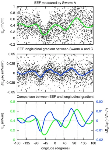
Due to the side-by-side constellation of the lower pair of Swarm satellites A and C, we are able for the first time to study longitudinal gradients of the EEF using near-simultaneous measurements. Figure 3 (top) shows the EEF data derived from Swarm A measurements as a function of longitude for local times between 1000 and 1200. This local time range corresponds to the time period May–June 2014, and so we cannot currently study the EEF at different seasons until more data are obtained. The green curve is a smoothed representation of the data computed from a moving average (over 100 points in longitude), and clearly demonstrates the longitudinal variability due to nonmigrating atmospheric tides which has been found in many equatorial ionospheric parameters [Immel et al., 2006; Forbes et al., 2008; Häusler et al., 2010]. In Figure 3 (middle), we show the longitudinal gradient ΔE_𝜙∕Δ𝜙, calculated by subtracting the two

Figure 3. (top) EEF estimated from Swarm A data as a function of longi-tude with moving average curve in green, (middle) Swarm A-derived EEF minus Swarm C-derived EEF divided by their longitudinal separation at the magnetic equator with moving average curve in blue, and (bottom) moving average curves for EEF (green) and longitudinal gradient (blue) shown on different vertical axes. All data are in local time sector 1000 to 1200.

near-simultaneous EEF estimates from satellites A and C and dividing by their longitudinal separation at the magnetic equator. The blue curve is a moving average (over 100 points in longitude) to smooth the data. We find gradients up to about 0.05 mV/m/deg in the longitudinal direction and also find periodic structure due to atmospheric tidal components. These instanta-neous gradient estimates correspond well with recent measurements of longitudinal vertical drift gradients determined from the Communications/ Navigation Outage Forecasting System (C/NOFS) satellite [Araujo-Pradere et al., 2011]. In a future study, we plan to perform a more detailed comparison of our gradient estimates with C/NOFS data to better gauge their accuracy and reliability.

In order to further verify that the Swarm EEF chain is able to correctly deter-mine these small-gradient signals, we plot in Figure 3 (bottom) the smoothed curve for the EEF derived from Swarm A (first vertical axis) and the corresponding curve for the longitudinal gradient computed from Swarm A and Swarm C (second vertical axis). A horizontal zero line is plotted in addition to vertical dotted lines to indi-cate where the gradient vanishes. We see that there is very good alignment between the vanishing gradient and extrema of the EEF curve.

4. Comparison With Independent Data Sets

The primary means of validating Swarm-derived equatorial electric field estimates comes from the JULIA (Jicamarca Unattended Long-term Investigations of the Atmosphere) radar system near Lima, Peru, which uses the Jicamarca array to measure coherent echoes from vertically propagating plasma depletions occur-ring near 150 km altitude [Kudeki and Fawcett, 1993]. While the physics behind these echoes is not well understood, their vertical velocities have been shown to be in good agreement with F region vertical drifts [Chau and Woodman, 2004]. The vertical drift velocity can then be directly translated into an eastward elec-tric field via the relation E = −v × B. Figure 4 shows comparisons of JULIA elecelec-tric field measurements with simultaneous satellite-derived EEF estimates. A simultaneous event is defined as when the satellite passes within 10◦longitude of the JULIA radar, and there exists a JULIA measurement within 5 min of the satellite pass. In Figure 4 (left), the Swarm EEF chain was used to process 10 years of CHAMP satellite Level-3 scalar magnetic data for comparison purposes. Using the above criteria, we found a total of 363 simultaneous measurements between CHAMP and JULIA. The correlation between E_CHAMPand E_JULIAis 0.78, and the best fit line is given by E_CHAMP= 0.96E_JULIA− 0.01 mV/m. Also shown in Figure 4 (left) are the Swarm-derived EEF estimates from all three satellites between November 2013 and October 2014. We found a total of 90 simul-taneous measurements for all three satellites. The correlation between ESWARMand EJULIAis also 0.78. The best

fit line is given by ESWARM = 1.08EJULIA+ 0.03 mV/m. Table 1 summarizes these statistics and also separates

Geophysical Research Letters

10.1002/2014GL062658

Figure 4. (left) Comparison of JULIA electric field measurements with CHAMP-derived EEF (2000–2010) and

Swarm-derived EEF (November 2013 to October 2014);y = xline shown as solid. (right) Comparison of Swarm-derived EEF with WAMNET SAM-MBOΔHmeasurements.

As can be seen from Table 1, the slopes of the best fit lines for Swarm satellites A and C are slightly larger than 1. It is unclear at present whether this is due to the small sample size, the climatological nature of the modeling, or if it is due to an unmodeled physical effect. As discussed in Alken and Maus [2010a], the slope of this line is heavily influenced by instabilities in the equatorial electrojet current stream (both gradient drift and two stream) which can reduce the current strength observed by the satellite, while leaving the electric field measured by JULIA unchanged. These instabilities are not modeled in our EEF chain; instead, an empirical correction factor is applied to the conductivity tensor to simulate the current reduction. Addition-ally, the longitudinal window taken around JULIA could introduce errors into the comparison. The longi-tudinal gradient in the EEF at Jicamarca is relatively large as seen from Figure 3 (about −0.01 mV/m/deg), and using a ±10◦window in longitude around JULIA could introduce errors up to 0.1 mV/m in the comparison. When more data are available, we will be able to shorten the longitudinal range to determine how the statistics improve.

As a second validation in a different longitude sector, we processed ΔH measurements from the WAMNET (West African Magnetometer Network) ground magnetic observatory chain for the time period 1 January to 28 February 2014. We use data from Samogossoni (SAM, 0.18◦N dip latitude, 11.60◦N, 5.77◦W, 351 m), situated very close to the magnetic equator, in combination with the International Real-time Magnetic Observatory Network (INTERMAGNET) observatories Mbour (MBO, 3.23◦N dip latitude, 14.39◦N, 16.96◦W, 7 m) and Tamanrasset (TAM, 11.35◦N dip latitude, 22.79◦N, 5.53◦E, 1373 m). Subtracting simultaneous measurements of the horizontal field component, using one observatory on the magnetic equator, and another a few degrees away in latitude, has been shown to be a good proxy of the EEJ current strength [Rastogi and Klobuchar, 1990; Alken et al., 2013a]. Before computing the ΔH between two magnetometer stations, we preprocessed the individual station data by fitting cubic splines to the nighttime (from 2200 to 0500 LT) horizontal component (H) time series of hourly values, which were then subtracted from all the data. This is designed to remove the main and crustal field baselines, typical quiet day variations occurring in

Table 1. Correlations Between Satellite-Derived EEF and JULIA orΔH Measurementsa

Correlation Correlation Correlation Satellite a b (mV/m) E_JULIA ΔH_MBO ΔH_TAM

CHAMP 0.96 −0.01 0.78

Swarm A 1.14 0.04 0.80 0.83 0.78

Swarm B 0.99 0.03 0.75 0.90 0.86

Swarm C 1.16 0.01 0.82 0.80 0.79

Swarm All 1.08 0.03 0.78 0.82 0.79

a_{The best fit line is given byE}

the magnetosphere, and possible instrument drift at the SAM station. Instrument drift is absent from defini-tive INTERMAGNET data. ΔH was then calculated by taking differences between the H component residuals of the SAM station on the dip equator and the MBO/TAM stations off of the dip equator. These differences were computed using the same universal time, which could introduce some error due to the longitudinal difference between SAM/MBO and SAM/TAM. We use the same criteria defined previously to identify simul-taneous measurements of ΔH and Swarm-derived EEF (maximum 10◦longitudinal separation with SAM and 5 min in time). Figure 4 (right) shows the comparison between ESWARMand the SAM-MBO ΔH

measure-ments. The right two columns of Table 1 list the individual correlations between the ESWARMand ΔH for both

SAM-MBO and SAM-TAM. We find in all cases a correlation of at least 78%, similar to the comparisons with JULIA, indicating that the Swarm EEF chain is also working well in the African sector.

5. Conclusion

The Swarm equatorial electric field inversion chain has been used to process nearly a year of Swarm ASM magnetometer data from November 2013 to October 2014. The ASM instrument is recording very good, low-noise signals of the equatorial electrojet, which are then being inverted by the EEF chain for estimates of the eastward equatorial electric field. The EEF estimates have been validated against independent measurements by the JULIA radar at Jicamarca, Peru. A total of 90 simultaneous measurements were recorded during this time period, with very good correlations and best line fits, comparable to statistical results found during the CHAMP satellite era. We also compare the Swarm-derived EEF with ΔH measure-ments from the WAMNET observatory network in West Africa, and find high correlations of at least 78% for all Swarm satellites.

We additionally report for the first time computations of longitudinal gradients in the equatorial electric field from near-simultaneous estimates of the EEF from the Swarm A and Swarm C lower satellite pair. We find longitudinal gradients of up to about 0.05 mV/m/deg which exhibit significant longitudinal variability, thought to be due to nonmigrating atmospheric tidal structure. To our knowledge, this work represents the first estimation of instantaneous longitudinal gradients in the EEF (and vertical drift velocities) at E region altitudes. These data will open the possibility of further study into the vertical gradients of upward drifting plasma, using measurements from the Ion Velocity Meter instrument on C/NOFS or the Electric Field Instrument on Swarm. Furthermore, these data will provide important inputs to theoretical and assimilative ionosphere models, providing a mechanism of comparing model results with day-to-day observations.

References

Alken, P., and S. Maus (2010a), Relationship between the ionospheric eastward electric field and the equatorial electrojet, Geophys. Res.

Lett., 37, L04104, doi:10.1029/2009GL041989.

Alken, P., and S. Maus (2010b), Electric fields in the equatorial ionosphere derived from CHAMP satellite magnetic field measurements,

J. Atmos. Sol. Terr. Phys., 72, 319–326, doi:10.1016/j.jastp.2009.02.006.

Alken, P., A. Chulliat, and S. Maus (2013a), Longitudinal and seasonal structure of the ionospheric equatorial electric field, J. Geophys. Res.

Space Physics, 118, 1298–1305, doi:10.1029/2012JA018314.

Alken, P., S. Maus, P. Vigneron, O. Sirol, and G. Hulot (2013b), Swarm SCARF equatorial electric field inversion chain, Earth Planets Space,

65(11), 1309–1317, doi:10.5047/eps.2013.09.008.

Anderson, D. N. (1981), Modeling the ambient, low latitude F-region ionosphere—A review, J. Atmos. Terr. Phys., 43(8), 753–762. Araujo-Pradere, E. A., D. N. Anderson, and M. Fedrizzi (2011), Communications/Navigation Outage Forecasting System observational

support for the equatorial E×B drift velocities associated with the four-cell tidal structures, Radio Sci., 46, RS0D09, doi:10.1029/2010RS004557.

Bilitza, D., L.-A. McKinnell, B. Reinisch, and T. Fuller-Rowell (2011), The International Reference Ionosphere (IRI) today and in the future,

J. Geod., 85, 909–920, doi:10.1007/s00190-010-0427-x.

Chau, J. L., and R. F. Woodman (2004), Daytime vertical and zonal velocities from 150-km echoes: Their relevance to F-region dynamics,

Geophys. Res. Lett., 31, L17801, doi:10.1029/2004GL020800.

Drob, D. P., et al. (2008), An empirical model of the Earth’s horizontal wind fields: HWM07, J. Geophys. Res., 113, A12304, doi:10.1029/2008JA013668.

Emmert, J. T., D. P. Drob, G. G. Shepherd, G. Hernandez, M. J. Jarvis, J. W. Meriwether, R. J. Niciejewski, D. P. Sipler, and C. A. Tepley (2008), DWM07 global empirical model of upper thermospheric storm-induced disturbance winds, J. Geophys. Res., 113, A11319, doi:10.1029/2008JA013541.

Fejer, B. G., and M. C. Kelley (1980), Ionospheric irregularities, Rev. Geophys. Space Phys., 18(2), 401–454.

Finlay, C. C., et al. (2010), International geomagnetic reference field: The eleventh generation, Geophys. J. Int., 183, 1216–1230, doi:10.1111/j.1365-246X.2010.04804.x.

Forbes, J. M. (1981), The equatorial electrojet, Rev. Geophys. Space Phys., 19(3), 469–504.

Forbes, J. M., X. Zhang, S. Palo, J. Russell, C. J. Mertens, and M. Mlynczak (2008), Tidal variability in the ionospheric dynamo region,

J. Geophys. Res., 113, A02310, doi:10.1029/2007JA012737.

Gagnepain, J., M. Crochet, and A. D. Richmond (1977), Comparison of equatorial electrojet models, J. Atmos. Terr. Phys., 39, 1119–1124.

Acknowledgments

The authors gratefully acknowledge support from the Centre National d’Études Spatiales (CNES) within the context of the “Travaux préparatoires et exploitation de la mission SWARM” project, and from the European Space Agency (ESA) through ESRIN contract 4000109587/13/I-NB “SWARM ESL.” The WAMNET magnetometer network is funded by CNES and is maintained by the Institut de Physique du Globe de Paris (IPGP), and the data are available at http://www. bcmt.fr/wamnetdata.html. The Jicamarca Radio Observatory is a facility of the Instituto Geofisico del Peru operated with support from the NSF through Cornell University. JULIA data are available at http://jro.igp.gob. pe/madrigal. Swarm Level-1b data are available from ESA at https://earth. esa.int/web/guest/swarm/data-access. The Swarm Level-2 EEF data will be made available shortly by ESA and can be made available upon request by the authors. The operational support of the CHAMP mission by the German Aerospace Center (DLR) is gratefully acknowledged, and CHAMP data can be downloaded from http:// isdc.gfz-potsdam.de. S.M. was sup-ported by NASA grant NNX13AL20G. This is IPGP contribution 3597. The Editor thanks Michael Kelley and an anonymous reviewer for their assistance in evaluating this paper.

Geophysical Research Letters

10.1002/2014GL062658

Häusler, K., H. Lühr, M. E. Hagan, A. Maute, and R. G. Roble (2010), Comparison of CHAMP and TIME-GCM nonmigrating tidal signals in the thermospheric zonal wind, J. Geophys. Res., 115, D00I08, doi:10.1029/2009JD012394.

Heelis, R. A. (2004), Electrodynamics in the low and middle latitude ionosphere: A tutorial, J. Atmos. Sol. Terr. Phys., 66, 825–838. Immel, T. J., E. Sagawa, S. L. England, S. B. Henderson, M. E. Hagan, S. B. Mende, H. U. Frey, C. M. Swenson, and L. J. Paxton (2006), Control

of equatorial ionospheric morphology by atmospheric tides, Geophys. Res. Lett., 33, L15108, doi:10.1029/2006GL026161. Kelley, M. C. (1989), The Earth’s Ionosphere: Plasma Physics and Electrodynamics, Academic Press, San Diego, Calif.

Kudeki, E., and C. D. Fawcett (1993), High resolution observations of 150 km echoes at Jicamarca, Geophys. Res. Lett., 20(18), 1987–1990. Maus, S., and H. Lühr (2005), Signature of the quiet-time magnetospheric magnetic field and its electromagnetic induction in the rotating

Earth, Geophys. J. Int., 162, 755–763, doi:10.1111/j.1365-246X.2005.02691.x.

Maus, S., F. Yin, H. Lühr, C. Manoj, M. Rother, J. Rauberg, I. Michaelis, C. Stolle, and R. D. Müller (2008), Resolution of direction of oceanic magnetic lineations by the sixth-generation lithospheric magnetic field model from CHAMP satellite magnetic measurements,

Geochem. Geophys. Geosyst., 9, Q07021, doi:10.1029/2008GC001949.

Onwumechili, C. A. (1997), The Equatorial Electrojet, Gordon and Breach Sci., Amsterdam.

Picone, J. M., A. E. Hedin, D. P. Drob, and A. C. Aikin (2002), NRLMSISE-00 empirical model of the atmosphere: Statistical comparisons and scientific issues, J. Geophys. Res., 107(A12), 1468, doi:10.1029/2002JA009430.

Rastogi, R. G., and J. A. Klobuchar (1990), Ionospheric electron content within the equatorialF₂layer anomaly belt, J. Geophys. Res., 95, 19,045–19,052.