HAL Id: hal-00295528
https://hal.archives-ouvertes.fr/hal-00295528
Submitted on 14 Sep 2004
HAL is a multi-disciplinary open access
archive for the deposit and dissemination of
sci-entific research documents, whether they are
pub-lished or not. The documents may come from
teaching and research institutions in France or
abroad, or from public or private research centers.
L’archive ouverte pluridisciplinaire HAL, est
destinée au dépôt et à la diffusion de documents
scientifiques de niveau recherche, publiés ou non,
émanant des établissements d’enseignement et de
recherche français ou étrangers, des laboratoires
publics ou privés.
particles in a global Eulerian model
M. M. P. van den Broek, J. E. Williams, A. Bregman
To cite this version:
M. M. P. van den Broek, J. E. Williams, A. Bregman. Implementing growth and sedimentation of
NAT particles in a global Eulerian model. Atmospheric Chemistry and Physics, European Geosciences
Union, 2004, 4 (7), pp.1869-1883. �hal-00295528�
www.atmos-chem-phys.org/acp/4/1869/
SRef-ID: 1680-7324/acp/2004-4-1869
Chemistry
and Physics
Implementing growth and sedimentation of NAT particles in a
global Eulerian model
M. M. P. van den Broek1, J. E. Williams2, and A. Bregman3
1Space Research Organization of the Netherlands (SRON), Utrecht, The Netherlands 2Eindhoven University, Eindhoven, The Netherlands
3Royal Netherlands Meteorological Institute (KNMI), De Bilt, The Netherlands
Received: 3 May 2004 – Published in Atmos. Chem. Phys. Discuss.: 16 June 2004
Revised: 8 September 2004 – Accepted: 8 September 2004 – Published: 14 September 2004
Abstract. Here we present a concise and efficient algorithm
to mimic the growth and sedimentation of Nitric Acid Tri-hydate (NAT) particles in the polar vortex in a state-of-the-art 3D chemistry transport model. The pstate-of-the-article growth and sedimentation are calculated using the microphysical formu-lation of Carslaw et al. (2002). Once formed, NAT particles are transported in the model as tracers in the form of size-segregated quantities or size bins. Two different approaches were adopted for this purpose: one assuming a fixed parti-cle number density (“FixedDens”) and the other assuming a discrete set of particle diameter values (“FixedRad”). Simu-lations were performed for three separate 10-day periods dur-ing the 1999–2000 Arctic winter and compared to the results of an existing Lagrangian model study, which uses similar microphysics in a computationally more expensive method for the simulation of NAT particle growth. The resulting particle sizes for both our approaches compare favourably at 430 K with those obtained from this previous model study, and also in-situ observations related to the size of large NAT particles. The particle growth is faster for “FixedDens” re-sulting in a difference in (de)nitrification by a factor of ∼ 2 for all three simulation periods. Comparisons were made with a standard equilibrium approach and the differences in the redistribution of HNO3were found to be substantial. For
both approaches the performance of the algorithm is rather insensitive to both the number of size bins and the shape of the size distribution, and show a weak dependence on the prescribed total particle number density during the coldest period. This results in an increase of 7% for the “FixedRad” approach and 17% for the “FixedDens” approach when in-creasing the total particle number density by a factor of 2.5.
Correspondence to: Miranda van den Broek
1 Introduction
Shortly after the discovery of the ozone hole in the mid 1980’s, it was recognized that denitrification (i.e. the uptake and subsequent sedimentation of HNO3within Polar
Strato-spheric Clouds, PSC’s) both increases and prolongs strato-spheric ozone loss (Crutzen and Arnold, 1986; Fahey et al., 1989; Fahey et al., 1990). Although this process is more prevalent and intense in the Antarctic winter stratosphere, as a consequence of lower temperatures, Shine et al. (2003) have conducted a recent comparison of stratospheric temper-ature changes and found that one possible outcome is that a future cooling could occur in the Arctic which would result in an increase in the importance of denitrification in the Arctic winter stratosphere. Moreover,during the last decade, obser-vational evidence of this vertical redistribution of HNO3 in
the Arctic stratosphere has also been found (e.g. Fahey et al., 1990; Sugita et al., 1998; Waibel et al., 1999), where it has been shown that such a redistribution can lead to an increase in Arctic ozone loss (Rex et al., 1997; Waibel et al., 1999).
More recently, during the Arctic winter of 1999/2000, which is one of the coldest currently on record (Manney and Sabutis, 2000), both extensive nitrification (Koike et al., 2002) and denitrification (Popp et al., 2001; Santee et al., 2000; Kleinb¨ohl et al., 2003) were observed. Again, large ozone loss was also derived for this winter using both model experiments (Sinnhuber et al., 2000) and in-situ ob-servations of ozone (Richard et al., 2001). Model results at-tributed 21–30% of ozone loss at the 460 K potential tem-perature level to denitrification (Davies et al., 2003). The presence of large HNO3-containing particles was recorded
directly by means of NOymeasurements on board the NASA
ER-2 aircraft (Northway et al., 2002a) and aerosol extinction measurements by the SAGE III satellite (Poole et al., 2003). The Multiangle Aerosol Spectrometer Probe (MASP) instru-ment took in-situ samples of large PSC particles (Fahey et al., 2001; Brooks et al., 2003). These particles ranged from
2–22 µm in diameter, with a bi-modal distribution. Since the sedimentation of large particles (>5 µm radius) is signifi-cantly faster than that of small particles, the presence of large particles increases the rate at which HNO3is redistributed.
To date, atmospheric models have typically described den-itrification using a rather simplified approach. For instance, most chemistry transport models (CTM’s) neglect to include PSC particles as transported species. Instead, a constant or equilibrium PSC particle size and number density are prescribed during the model runs (e.g. Chipperfield, 1999; Koike et al., 2002). Several of these model studies have concluded that such a simple parameterization of denitri-fication maybe inadequate for modelling Arctic wintertime ozone loss (Kleinb¨ohl et al., 2003; Sinnhuber et al., 2000). Therefore, agreement between model results and observa-tions may simply be fortuitous. For instance, Koike et al. (2002) were able to represent NOy measurements
dur-ing the 1999/2000 winter with a CTM usdur-ing an average NAT particle radius of 5 µm and fixed particle number density of 5×10⁻³cm−3. Although this radius falls within the range of observed radii for large particles, the particle number den-sity was overestimated by a factor of ∼20 (c.f. Fahey et al., 2001). Thus, the finding that large NAT particles ex-ist with correspondingly low particle number densities has introduced a strong constraint regarding the description of NAT particles in atmospheric models. A proper description of NAT particles is essential to modelled ozone loss in a cool-ing stratospheric climate. It has been demonstrated that cur-rent CTM’s significantly underestimate the temperature sen-sitivity of ozone loss during the last two decades (Rex et al., 2004). This partly reflects shortcomings in NAT represen-tation in global chemistry climate or transport models. Cer-tain non-equilibrium model studies have been carried out for the same winter. For example, Jensen et al. (2002) used 1-D model simulations of NAT growth and transport. They tested the sensitivity of the model results towards a num-ber of input parameters, of which the lifetime of the NAT cloud was found to be the most important. The first 3-D model study to include non-equilibrium growth and simul-taneous sedimentation of NAT particles was that of Carslaw et al. (2002), where a Lagrangian microphysical algorithm was coupled to the SLIMCAT CTM for particle transport. This study was unique in that the authors were able to rep-resent the radii of the large particles measured by Fahey et al. (2001). This algorithm was also used in combination with the CTM to simulate the entire 1999/2000 winter and yielded results for denitrification that were consistent with observations (Mann et al., 2003). One disadvantage of us-ing a Lagrangian method for simulatus-ing NAT particles is that the algorithm is prohibitively expensive for multiple year or long-term climate runs when using CTM’s or GCM’s (Gen-eral Circulation Models). Therefore, the development of a concise, computationally efficient method, which transports NAT mass according to size, is required but has yet to be developed. In this paper we aim to address this issue by
in-troducing a computationally inexpensive algorithm designed for use in CTM’s, describing nonequilibrium growth, sedi-mentation of NAT particles and subsequent transport of the size-segregated particles as chemical tracers, following the parameterization developed by Carslaw et al. (2002). We will show consistent results from two different approaches describing growth and transport of NAT, which both yield realistic HNO3redistribution, NAT particle sizes and
parti-cle number densities. In Sect. 2, the CTM and the algorithms for both approaches are described. Sect. 3 shows the results in comparison to observations and other model studies. Sev-eral sensitivity studies are carried out and described in Sect. 4 and, finally, the discussion and conclusions are presented in Sect. 5.
2 Model description
2.1 The TM5 model
For our purpose we use the recently developed global three-dimensional transport model, version 5 (TM5). This model has been used previously for several studies of both the tro-posphere (e.g. Krol et al., 2004; Krol et al., 2003) and strato-sphere (van den Broek et al., 2003). It has been developed by modification of the existing TM3 model, which has also been used for a number of stratospheric chemistry and transport studies (van den Broek et al., 2000; Bregman et al., 2000; Bregman et al., 2001). The main improvement is the inclu-sion of a zooming algorithm and the vertical exteninclu-sion of the model domain up to 0.2 hPa, with a higher vertical resolution. In this study we apply a 2◦latitude by 3◦longitude
horizon-tal resolution for all model runs. The transport of tracers in TM5 is driven by six-hourly forecast fields for temperature, surface pressure, wind, humidity and convective mass flux taken from the European Centre for Medium-Range Weather Forecasts (ECMWF) operational data. The method to cal-culate mass fluxes from ECMWF winds has recently been improved (Bregman et al., 2003). We used a 33-layer sub-set of the 60 layer fields that are taken into account in the ECMWF model, with a reduced number of levels in the tro-pospheric boundary layer and above 70 hPa. Near the surface the model levels are defined as terrain following sigma coor-dinates whereas the layers above 100 hPa are defined at pres-sure surfaces. A hybrid of the two is used between the lower troposphere and the lower stratosphere. The mass flux advec-tion scheme contains first order slopes (Russell and Lerner, 1981) or second-order moments (Prather, 1986). A model time step of 1800 s is applied, resulting in dynamical and chemical time steps of 900 s. In contrast to previous model configurations of TM3 and TM5 no reduced grid is applied in the polar region. Instead, the time step in the advection scheme is decreased iteratively to prevent violation of the Courant Friedrichs-Lewy (CFL) condition (Bregman et al.,
20041). To focus solely on the redistribution of HNO3 and
performance of the NAT algorithm in this theoretical study no gas phase chemistry was active for any of the runs. This allows us to compare the results with those of Carslaw et al. (2002). Nitric Acid Dihydrate (NAD) is not accounted for as it is thought to result in a small effect in terms of NOy
redistribution when temperatures fluctuate around 190 K due to the associated higher HNO3equilibrium pressure (Jensen
et al., 2002). For the Arctic vortex, the coldest temperatures typically only fall to the values needed for NAD formation for a few days, therefore NAD particles never grow to ap-preciable sizes and thus do not sediment. No supercooled ternary solution (STS) is included as to avoid the transport of additional tracers (i.e. H2SO4and liquid aerosol). The
ini-tial profiles used for HNO3and H2O were set at 8 ppbv and
5 ppmv, respectively, for the entire column in all runs, simi-lar to those used for the Lagrangian study by Carslaw et al., 2002. This [HNO3] in the stratosphere is based on extensive
measurements (Kleinb¨ohl et al., 2003) and considered to be a lower limit for the average stratospheric [HNO3] available.
2.2 The algorithm for NAT growth and sedimentation The key aspect of our algorithm is the calculation of NAT particle growth in combination with the transport of NAT as tracers that are segregated by size. This is done by distribut-ing the NAT particles between a number of size bins. The particle number density per size bin (nbin, cm−3) and
parti-cle radius (r, m) define the NAT mass according to Eqs. (1) and (2):
mp =
[NAT] nbin
, (1)
where [NAT] is the concentration of NAT (g cm−3), and mp
is the mass (g particle−1) r3= mp
ρNAT · 3
4π, (2)
where ρNATis the density of NAT=1.626×10⁶g m−3(Drdla
et al., 1993).
To implement the exact calculation of the NAT properties within an Eulerian model, the advection of another model property, besides mass, would be required, e.g. the NAT
number density. This would however result in a double
amount of tracers, thereby dramatically decreasing the model efficiency. Furthermore, the separate transport of two quan-tities that are linked to each other, but are allowed to have different model gradients, will give severe numerical prob-lems during advection. For example, a number density of NAT could exist in a model grid box while no mass of NAT is present. Therefore, we have only included the transport of NAT mass while assumptions are made regarding the particle number density per size bin (nbin)or the radius (r). Firstly,
1manuscript in preparation
NAT formation in first size bin at Tnat at initial conditions
NAT growth is calculated for each size bin NAT in
first size bin? No NAT in
TM5
T < 200 K? Lat > 50 deg N?
Radius and number density are calculated
from NAT mass HNO3
concentra-tion is adapted
Sedimentation is calculated
Redistribution of particle mass over the size bins
Radius or number density is re-calculated from NAT mass
Advective transport of NAT size bins and HNO3 1 2 3 4 5 6 7 8 YES YES NO
Fig. 1. Schematic diagram for the calculation of growth and
sedi-mentation of NAT particles using the “FixedRad” and “FixedDens” algorithms. The black text indicates the general approach, whereas the red text indicates differences between approaches “FixedRad” and “FixedDens”. See Sect. 2.2 for more details.
we introduce an approach that assumes a fixed nbinper size
bin (hereafter referred to as “FixedDens”). Secondly, we in-troduce an approach that assumes that each particle that re-sides in a specific size bin has the average radius for that size bin (hereafter referred to as “FixedRad”). In contrast to these two nonequilibrium approaches, we also discuss the equi-librium approach, which is adopted by most previous model studies (e.g. Koike et al., 2002).
The process of NAT particle growth and sedimentation within TM5 is clarified in the schematic given in Fig. 1. Any differences that occur between “FixedDens” and “FixedRad” are denoted in red. These differences are described in more detail in Sects. 2.3 and 2.4. The schedule is valid for each model grid box in which temperature is low enough for the presence of NAT. Both approaches describe the formation of NAT, particle growth/evaporation, particle sedimentation and the particle size spectrum in an identical manner. NAT par-ticles are allowed to exist in the model only when tempera-ture ≤200 K and latitude >50◦N. After initialization of the model, fresh formation of NAT particles only occurs if the first size bin is empty.
In most CTM’s, NAT formation is assumed to occur either on ice particles (e.g. Kleinb¨ohl et al., 2003) or at supersatu-ration of the surrounding HNO3-containing air with respect
to NAT, usually by a factor of 10 (e.g. Koike et al., 2002). The exact formation mechanism of NAT has still not yet been fully elucidated from the detailed microphysical studies that have been performed, meaning there is still some debate re-garding NAT formation (Drdla, 2003; Knopf et al., 2002; Tabazadeh et al., 2003). For this reason we adopt a sim-ple approach where, in the base run of our model, particles
initially form in the first size bin with a radius of 0.1 µm and a particle number density of 5.75×10⁻⁵cm−3(process 1 in
Fig. 1) when the temperature is below the NAT equilibrium temperature TNAT(Hanson and Mauersberger, 1988). Both a
doubling of the initial radius and enlarging the threshold for NAT formation by assuming a super saturation by a factor of 10, made no significant change to our results (not shown).
The growth and evaporation of NAT is calculated using the algorithm adopted from Carslaw et al. (2002) (process 2 in Fig. 1). Before implementation of this algorithm into a 3D model run, we first tested the formulation using a box model and successfully reproduced the particle sizes and sedimen-tation rates for NAT (not shown) as those shown in Carslaw et al. (2002). An assumption we make is that the calculation of growth across all size bins starts with the smallest size bin. After growth, the NAT particles are re-binned across the size spectrum, meaning that the mass distribution also changes accordingly (process 3 in Fig. 1). The assumptions used re-garding the calculation of r and nbinfrom the NAT mass are
different in both methods and are explained in more detail in Sects. 2.3 and 2.4, below. After the re-binning step, a stoichiometric 1[HNO3]gis calculated according to the
in-crease or dein-crease of NAT in each grid box (process 4 in Fig. 1). Since both r and nbinare needed for the calculation
of the sedimentation rate, differences occur between both ap-proaches (process 5 in Fig. 1), before sedimentation is de-scribed (process 6 in Fig. 1). Numerical diffusion due to ver-tical layering is limited by applying first-order slopes(Russell and Lerner, 1981) to the sedimentation calculation. The cal-culation of NAT growth and sedimentation is followed by the advective transport of all tracers, i.e. HNO3and the NAT
mass per size bin (process 7 in Fig. 1). After this advective transport of the modelled species the NAT growth subroutine starts again with the calculation of either r (“FixedDens”) or nbin(“FixedRad”) from the transported NAT mass (process 8
in Fig. 1).
2.3 The “FixedDens” approach
In this approach r is calculated for each respective size bin from the transported particle mass and the constant nbin
value, by using Eqs. (1) and (2). This means that we need to assume that nbinremains constant for each size bin across
the entire size bin spectrum after the initial formation of NAT particles. All particles within the same size bin are assumed to grow or evaporate by the same amount. After NAT growth, re-binning of the particles occurs if 1r is large enough for the size bin limit to be exceeded. During this process, the mass of NAT is conserved.
A drawback of this method is that a constant size distri-bution is applied, whereas in reality the size distridistri-bution will change during the growth and evaporation of the NAT parti-cles. Since the radius r is related to nbinthrough the
parti-cle mass (Eqs. 1 and 2), an underestimated nbinmay lead to
an overestimation of r, or the reverse. To diminish this
ef-fect, we chose nbinso that the total number density summed
across all bins is in close agreement with observed values of large particles (Fahey et al.,2001) after a 10-day simulation. The effect of these assumptions have been investigated using several sensitivity studies and the findings are discussed in Sect. 4.
2.4 The “FixedRad” approach
In this second approach the nbinof each size bin is calculated
using the transported particle mass together with Eqs. (1) and (2). Here, we assume that the NAT particle radius (r) equals the average radius of each respective size bin. To allow the transfer of particles between size bins an nbinthreshold is
re-quired, otherwise an explosion of small particles occurs as a consequence of resetting r equal to the average bin radius at each time step. The time step required to solve this nu-merical problem would have to be unrealistically small . Par-ticle growth and sedimentation are calculated in an identi-cal manner as for the “FixedDens” approach. After growth, any 1r is immediately converted into an increase in nbin
us-ing the associated increase in NAT mass (see Eqn. 2). If the re-calculated nbinexceeds the nbinthreshold for any
partic-ular size bin then the excess nbinis transferred (as mass) to
the next size bin. During this step mass is conserved, lead-ing to an instantaneous reduction in the transferred nbinas a
consequence of the instantaneous increase in r, which is set equal to the bin average. This continues until the NAT par-ticulate mass resides across the entire size bin spectrum. An advantage of this approach is that a realistic size distribution, with nbinchanging per size bin, may be introduced into the
scheme. In the “FixedDens” scheme this would introduce a fluctuation in the number of particles during transfer across the size bins, either introducing a mass inconsistency or an artificial change of the radius. Moreover, only a fraction of the particles resident within one size bin need to move to the next size bin upon particle growth. However, an associated disadvantage is that the growth or evaporation of particles is actually calculated as a change in nbin instead of r, in the
first instance, introducing some diffusivity in the size spec-trum. Whereas the nbin thresholds move the particles
up-ward to the next size bin during a period of growth, continual evaporation would result in a very small nbinvalue, which
essentially indicates the emptying of the size bin. Combined with the advective transport of particles, the result of the nbin
thresholds is that not all size bins are at the nbinlimit at any
one time and location, which is more realistic than the as-sumption of constant nbinin the “FixedDens” method. The
assumption that the radius of resident NAT particles in any size bin equals the average radius of that size bin has some influence on the particle growth. Depending on whether nbin
represents a NAT mass above or below the average r, a small over- or underestimation of growth may occur. Several sen-sitivity studies to assess the impact of these assumptions are discussed in Sect. 3.
Fig. 2. Minimum temperatures in the ECMWF 6-h forecasts on the
380 K and 475 K potential temperature levels during January and February 2000. The three integration periods are indicated with the shaded areas.
2.5 Equilibrium approach
To date, CTM models have adopted a simplified way to pa-rameterize denitrification. Typically, a constant r and nbinof
NAT are prescribed (Chipperfield et al., 1999; Koike et al., 2001), or alternatively, calculated assuming an equilibrium particle size (Sinnhuber et al., 2000; Davies et al., 2003). In all these studies, NAT mass is not transported and it is deter-mined at each time step whether NAT formation is possible. This is in strong contrast to the nonequilibrium methods in-troduced above, which allow the NAT particles to grow and be transported within a fixed number of size bins.
To allow a direct comparison to be made between all the methods discussed here, we performed two model runs using such a simplified approach, which we refer to as the equilib-rium approach.
3 Description of the model runs
3.1 Simulation period
Model runs were carried for three separate 10-day time inter-vals during the 1999/2000 winter period, these being 10–20 January, 24 January–3 February and 16–26 February, respec-tively. The end dates of these periods coincide with the NAT
particle observations made by the NOAA NOy and MASP
Table 1. Prescribed radii size limits, average radius, size bin
par-ticle density (nbin)and number concentrations used for the base
run. Values are given for each respective bin. Within the “Fixed-Dens” approach, nbinis fixed, whereas the “FixedRad” approach
uses them to set mass thresholds for each bin (see Sect. 2.4). Simu-lations were performed for all chosen time intervals (see Sect. 3.1) using each approach.
Size bin number 1 2 3 4 5 Minimum r (µm) 0 0.2 2 6 12 Maximum r (µm) 0.2 2 6 12 25 Average r (µm) 0.1 1.1 4 9 18.5 Number density per
size bin (10−5cm−3) 5.75 5.75 5.75 5.75 5.75 Number concentration
(10−5cm−3µm−1radius) 28.75 3.194 1.4375 0.958 0.442
instruments (Fahey et al., 2001; Brooks et al., 2003) and also allow us to make a direct comparison with the results of a Lagrangian modelling study of NAT formation for identical periods (Carslaw et al., 2002). Figure 2 depicts the minimum temperatures from the ECMWF 6-h forecast fields at two po-tential temperature levels, 380 K and 475 K, during this win-ter. From there it can be seen that the minimum temperature at 475 K is continuously below 193 K, which approximately equals TNAT, during the first two simulation periods. The first
period, 10–20 January, experienced the coldest stratospheric temperatures of all the three chosen intervals with T <191 K throughout the period at 475 K.
3.2 The base run
A base run was defined to allow a direct comparison to be made between the two methods introduced in Sects. 2.3 and 2.4. During this run NAT was formed at the NAT equilib-rium temperature (Hanson and Mauersberger, 1988) with an initial radius of 0.1 µm. Once formed, no selection crite-ria were used during the growth of particles meaning that all particles in a specific size bin grow by the same extent during a particular time-step. In total 5 size bins were de-fined with the thresholds used for each size bin being shown in Table 1. The minimum, maximum and average r val-ues,along with the number concentrations assumed for each bin, are also given for both methods. Initial tests implied that this number of bins equalled the minimum number of tracers needed to achieve a reasonable amount of reparti-tioning of HNO3.The nbinvalues for each bin were chosen
such that the permissible sum of the particle number con-centrations for particle sizes of r<10 µm could never exceed 2.3×10⁻⁴cm−3, which is in line with the number densities of large particles observed by Fahey et al. (2001) during the same Arctic winter. This meant a maximum particle number
Table 2. Definition of the sensitivity runs conducted regarding the number of size bins, the total particle number density at the end of the
simulation, the particle number concentrations in each bin (nbin), and the initial diameter.
Definition of No. size Total particle Number density Initial the model run bins number density per size bin nbin diameter (µm)
(1×10⁻⁴cm−3) (1×10⁻⁵parts cm−3)
I Base 5 2.3 5.75 0.2
II Equilibrium a. 0 2.3 N/A 14.5
b. 0 2.3 N/A 8.0
III Number density 5 0.4–4 1–10 0.2 IV Number of bins 5–18 2.3 1.60–5.75 0.2
(see Figs. 3a–3d)
V Size spectrum 7 2.3 Varying 0.2 (see Fig. 3e)
density of 5.75×10⁻⁵cm−3could exist for any of the first 4 size bins. For NAT particles with r>10 µm the fifth bin was introduced to ensure model stability (i.e. to account for any overflow from the 4th bin). For a comprehensive descrip-tion of how the nbin values are used in each approach the
reader is referred to Sects. 2.3 and 2.4 above.The black line in Fig. 3a shows the maximal size distribution allowable in the base run.
3.3 Sensitivity studies
To investigate the stability, performance and constraints of both approaches, a series of sensitivity tests were performed and the resulting denitrification was examined. All sensi-tivity studies were performed for the first 10-day interval of 10–20 January 2000, where the unusually low tempera-tures ensured the existence of NAT particles in the model for the entire simulation period. The sensitivity studies can be grouped into four main categories: (i) comparison against an equilibrium model which neglects NAT growth and trans-port, (ii) the influence of the nbinlimit, (iii) the influence of
the number of size bins (and thus tracers) and (iv) the influ-ence of differently shaped size spectra. Details regarding the constraints of the sensitivity runs are given in Table 2 be-low, while the related maximum possible size distributions are shown in Fig. 3. Figure 3a shows the maximum possible size distribution of the base run (black line) plus those used for the sensitivity tests with higher (blue) and lower (red) to-tal number densities, which are discussed in Sect. 4.2.2. The maximum permissible size distributions for the runs with 7, 10 and 18 size bins are shown in Figs. 3b–d, respectively, and their results are discussed in Sect. 4.2.3. Figures 3e–g show the differently shaped maximum size distributions, where each uses 7 bins and the maximum possible total number density equals 2.3×10⁻⁴cm−3for r<10 µm, identical to the base run. The subsequent results are discussed in Sect. 4.2.4.
4 Results
4.1 The base run
4.1.1 Particle sizes
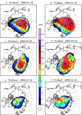
Figures 4a, c and e show the average diameter per grid box on the θ =430 K level after a 10-day model run using the “Fixed-Dens” approach for 20 January, 3 February and 26 February, respectively. We have chosen this format so that direct com-parisons can be made with similar figures shown by Carslaw et al. (2002) for the same periods. Here, the average diame-ter ( ¯d)is obtained by weighting the diameter of particles that reside in each respective size bin with the mass fraction of total NAT (hereafter referred to as [NAT]tot)present in each
size bin according to Eq. (3): ¯ d =Xn=ntot n=1 ¯ dn· [NAT]n [NAT]tot , (3)
where n= the size bin number and ntot is the total size bin
number.
The largest particles form during the first period, where the minimum vortex temperature is continuously below 191 K at θ=475 K (see Fig. 2). The maximum ¯d values obtained for the first period in the “FixedDens” run range from 18–20 µm, which is comparable to the maximum particle diameter mea-sured by the MASP instrument (∼20 µm) on the same day at approximately the same altitude (Fahey et al., 2001). The model results of Carslaw et al. (2002),which were obtained by applying the same growth/sedimentation algorithm in a Lagrangian model, show somewhat smaller particle sizes, with a maximum diameter of 16–18 µm at between θ =420– 440 K (c.f. Fig. 2 in Carslaw et al., 2002). It should be noted that the particle number concentrations at this θ level are lower than those obtained by Carslaw et al. (2002) by ≥50% across the entire size spectrum as a consequence of fixing the particle number density for each size bin in the “Fixed-Dens” approach (c.f. Fig. 3 in Carslaw et al., 2002). This has
Fig. 3. Plots of particle number concentration (cm−3µm−1) versus particle diameter (µm) for all sensitivity runs performed for the “Fixed-Dens” and “FixedRad” approaches: (a) base run (black), with the higher (blue, 4×10⁻⁴cm−3)and lower (red, 4×10⁻⁵cm−3)total number density spectra overlaid, (b) 7 bins, (c) 10 bins, (d) 18 bins, (e) and (f) 7 bin model run with differently shaped size distributions: negative (blue) and positive slope (red) and observed (by Fahey et al., 2001) distribution (green) (see Sect. 4.2.2 for more details). The total number density for runs (b–g) was similar as for the base run.
a. "FixDens", 2000-01-20 b. "FixRad", 2000-01-20 f. "FixRad", 2000-02-26 e. "FixDens", 2000-02-26 d. "FixRad", 2000-02-03 c. "FixDens", 2000-02-03 24 22 20 18 16 14 12 10 8 6 4 2 0.2 µm
Fig. 4. Grid box average NAT particle diameters (µm) on the
θ=430 K level, after 10-day simulations with the end dates 20 Jan-uary, 3 February and 26 FebrJan-uary, using both the “FixedDens” and the “FixedRad” approaches. A comparable figure is shown by Carslaw et al. (2002, Fig. 2), who applied a Lagrangian model of NAT growth and transport for identical periods.
consequences regarding the growth rate of the NAT particles (see Sect. 4.2.2.). For the other simulation periods, which ex-perienced higher temperatures and thus less NAT formation, the maximum ¯dvalues are smaller than those obtained in the first period by 1-5µm. This results in a larger absolute dif-ference with Carslaw et al. (2002) when comparing particle diameter sizes for the respective end dates, 3 and 26 Febru-ary. These differences in maximum ¯dusing the “FixedDens” approach and those obtained by Carslaw et al. (2002) we feel are acceptable, considering the difference in the treatment of particle transport and the large uncertainties associated with both the particle number density and size distribution.
Figures 4b, d and f show the corresponding plots of the ¯
d values when using the “FixedRad” approach for identi-cal dates. For the first interval ¯d is somewhat smaller than that obtained for the “FixedDens” run, with the maximum ¯d being ∼18 µm. However, the difference in maximum ¯d in-verses between the two approaches for the second simulation period, with the “FixedRad” approach having a maximum ¯d
value 0.4µm larger than the corresponding “FixedDens” run (c.f. Figs. 4c with d). Moreover, for the third period the dif-ference in ¯dis even larger, with the “FixedRad” approach ex-ceeding the “FixedDens” by 3µm (c.f. Figs. 4e with f). The integrated area over which large NAT particles are present is generally larger for the “FixedRad” runs compared to the “FixedDens” runs. However, even though larger particles ex-ist over a wider area, the actual number of such particles can be rather small (e.g. the mass of the second largest particles, NAT tracer number 4, is between 0–100 pptv at pressures <30 hPa). In fact during the analysis of the data a filter was applied to Eq. (3) to avoid including extremely small (NAT) concentrations. When the NAT total number density was less than 5×10⁻⁹cm−3the data were effectively ignored. Three separate effects are responsible for the observed differences between both approaches. For the first period the differences originate mostly from the particle size discretization which occurs in the “FixedRad” approach. During cold periods, where strong particle growth occurs, the radius is artificially reduced towards the average bin radius at the start of each time-step (i.e. the rate of particle growth is slowed) whereas for the “FixedDens” approach any increase in radius is pre-served between time-steps. This results in larger particles occuring for the “FixedDens” approach after 10 days of sim-ulation. [JEW: The second effect is more important for the second and third periods, where the temperatures fluctuate around the NAT formation temperature, thus evaporation of NAT mass occurs for selected days. In the ”FixedDens” ap-proach, this evaporation manifests itself as a reduction in the size of all particles in each respective size bin, resulting in a lower ¯d value. For ”FixedRad” ,the loss of NAT mass re-sults in lower nbinvalues across the entire range of size bins.
This results in a smaller decrease in the ¯d values. The third effect, which is the effect of atmospheric mixing processes, accentuates such changes on ¯d in both approaches for sim-ilar reasons. The particle transport results in a dilution of the NAT mass between time-steps which affects the nbinfor
“FixedRad” and r for “FixedDens”, as governed by their def-initions. The cumulative effect of all three influences results in larger NAT particle sizes for “FixedRad” on the second and third end dates.
Figures 5a and b show the development of the largest ¯d values in the vortex over the entire 10-day simulation pe-riod between 10–20 January 2000 for both approaches, with 1t=12 h. By analysing the results in this way such plots highlight the growth rate and sedimentation of the largest NAT particles with respect to time. The plot starts 12 h af-ter initialization of the model. Within two days, maximum particle sizes between 10–12 µm diameter are reached at a pressure level of 25 hPa. This is comparable with the findings from the box model by Carslaw et al. (2002), who calculate particles with a diameter of 10 µm after 2 days, starting at the same altitude and HNO3mixing ratio, with a
ture of 188 K. The coinciding lowest atmospheric tempera-ture during the first two days of our runs is somewhat lower,
12 14 16 18 20 100
10
b. "FixRad", NAT diameter, 10-20 Jan 2000
Day of the year 2000
12 14 16 18 20
100 10
a. "FixDens", NAT diameter, 10-20 Jan 2000
Day of the year 2000
Pressure [hPa] Pressure [hPa] 24 22 20 18 16 14 12 10 8 6 4 2 0.2
Fig. 5. Vertical cross section of the grid box average particle
diam-eter ¯d(µm). At each time (12-hour intervals) and altitude during the 10-day simulation between 10-20 January the vortex maximum
¯
dis plotted for (a) “FixedDens” and (b) “FixedRad”
i.e. 185 K, which may explain the slightly larger particle sizes in our runs. Extremely large ( ¯d>22 µm) particles are found at the bottom of the vortex for both approaches. However, it should be noted that a constant HNO3mixing ratio of 8 ppbv
was applied for these simulations, which is unrealistically high in the lower stratosphere.
By comparing Figs. 5a and b, several striking differences become evident between both of the approaches. Firstly, the initial growth occurs faster for the “FixedRad” approach (e.g. by the end of the second day the maximum particle diame-ter at 50 hPa reaches 14—16 µm for “FixedRad” whilst the corresponding value for “FixedDens” is 12–14 µm) Over the next few days, particle growth then slows down for “Fixe-dRad” resulting in larger particle sizes for “FixedDens”. Sec-ondly, “FixedDens” exhibits a more stratified set of ¯dvalues as a consequence of the particle radii being allowed to vary across a wider range of values.
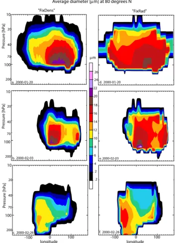
Figure 6 clearly illustrates the differences which occur in the vertical distribution of particle sizes between both the ap-proaches by showing ¯dat 80◦N on the end date of each cho-sen simulation period. Comparing Figs. 6a and d it can be
100 200 10 20 40 70 100 200 10 20 40 70 100 200 10 20 40 70 longitude -100 0 100 longitude -100 0 100
Average diameter [mm] at 80 degrees N
"FixRad" "FixDens" a. 2000-01-20 d. 2000-01-20 b. 2000-02-03 c. 2000-02-26 e. 2000-02-03 26 24 22 20 18 16 14 12 10 8 6 4 2 .2 mm Pr es su re [h Pa ] Pr es su re [h Pa ] Pr es su re [h Pa ] f. 2000-02-26
Fig. 6. Vertical cross section at 80◦N of the grid box average NAT particle diameter (µm) after 10-day simulations with the end dates 20 January (a+d), 3 February (b+e) and 26 February (c+f), using both the “FixedDens” (a–c) and the “FixedRad” (d–f) approaches.
seen that the area of large NAT particles is more extensive in the “FixedRad” approach even though the largest particle size occurs for “FixedDens” (c.f. Figs. 4a and b). In line with the Fig. 4., Fig. 6 shows that for the end dates of the second and third period larger particles occur for “FixedRad”. As explained above, this effect can be attributed to the different treatment of NAT evaporation and atmospheric mixing be-tween both approaches. Further, it is interesting to note that the base level at which NAT occurs drops with respect to the simulation date due to descent of air within the vortex. 4.1.2 Denitrification
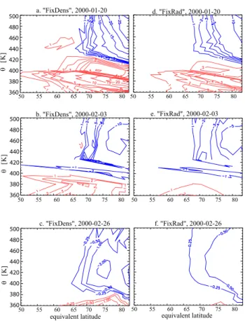
Figure 7 shows a direct comparison of the percentage change in HNO3calculated by each of our methods against
equiva-lent latitude for the three chosen simulation periods. Here, (de)nitrification is shown on potential temperature levels, against equivalent latitude.
The 10–20 January model run results in the greatest 1HNO3 of all three chosen simulation periods, with the
q [ K ] q [ K ] q [ K ]
equivalent latitude equivalent latitude
50 55 60 65 70 75 80 50 55 60 65 70 75 80 a. "FixDens", 2000-01-20 b. "FixDens", 2000-02-03 c. "FixDens", 2000-02-26 e. "FixRad", 2000-02-03 f. "FixRad", 2000-02-26 50 55 60 65 70 75 80 50 55 60 65 70 75 80 d. "FixRad", 2000-01-20 50 55 60 65 70 75 80 50 55 60 65 70 75 80 500 480 460 440 420 400 380 360 500 480 460 440 420 400 380 360 500 480 460 440 420 400 380 360
Fig. 7. The percentage (de)nitrification on potential temperature
θ against equivalent latitude for (a+d) 20 January 2000, (b+e) 3 February 2000 and (c+f) 26 February 2000. The left column shows the results for the “FixedDens” approach, the results for the “Fixe-dRad” approach are shown on the right.
maxima being ∼10 and ∼25% for “FixedRad” and “Fixed-Dens”, respectively (c.f. Fig. 7a and d) due to the persis-tence of unusually low temperatures allowing the growth of large particles. For the second period, between 24 January–3 February, denitrification is somewhat lower, with the corre-sponding maxima being ∼5 and ∼10% (c.f. Figure 7b and e). For the final period, between 16–26 February 2000, practi-cally no (de)nitrification is predicted by both approaches, de-spite the maximum ¯dbetween 12–16 µm that was calculated for the end dates (c.f. Figs. 4e, f, 6c and f). (De)nitrification in the second and third periods also occurs at lower θ levels compared to the first simulation period as a consequence of the descent of the coldest region in the vortex (see Fig. 2).
For all periods, “FixedDens” results in much more (de)nitrification than “FixedRad” by a factor of ∼2. This is due to the faster rate at which larger particle sizes occur when using the “FixedDens” approach which allows more repartitioning of HNO3as a result of the particles falling
fur-ther. However, it should be noted that the limited period over which these simulations were performed restricts the conclu-sions which maybe drawn when integrating over an entire winter.
4.2 Sensitivity studies
As discussed in Sect. 3.2, a number of prescribed model pa-rameters were used for the base run simulation, where the choice of such parameters could influence performance of the algorithms to describe NAT growth and transport. For this reason we have tested the model sensitivity towards such parameters to quantify the robustness of our approaches. The simulation period of 10–20 January was used exclusively for this purpose due to the occurrence of large NAT particles as described earlier. The prolonged period of low temperatures also ensures that NAT was present throughout the entire pe-riod, making differences between the sensitivity runs more easily discernible. For brevity we limit our discussion to the main categories as defined in Sect. 3.3. In addition, we have also tested several other model parameters which resulted in negligible differences in NOyre-distribution for both
meth-ods, these being: the number of vertical layers used in the model; the type of advection scheme employed (first order or second moments); doubling the radius of the initial size bin, i.e. the nucleation rate; and increasing the supersatura-tion of HNO3 needed for NAT formation to 10. It should
be noted that these results pertain to a chemically passive version of TM5 and the sensitivity should be re-tested when adding chemical tracers.
4.2.1 Comparison with the equilibrium approach
To allow a direct comparison of the equilibrium method with the base runs, the total particle number densities and radii for all NAT particles were set constant in two different runs. For the first sensitivity run, the number density and radius were 2.3×10⁻⁴cm−3and 7.25 µm, respectively, which equals the
average values found by Fahey et al. (2001). These sizes were observed on 20 January after a persistent cold period. Since the equilibrium approach assumes a constant radius, using the observed radius throughout the integration period may overestimate denitrification. Therefore, smaller radii were assumed in the second sensitivity run, i.e. 4 µm. Again, NAT formation was calculated using TNATbased on the
Han-son and Mauersberger criterium (1988) at each model time step (900 s). Figures 8a–d show the vertical redistribution of total HNO3at 80◦N latitude across all longitudes for the
“FixedDens”, “FixedRad” and both equilibrium runs, respec-tively. From Fig. 7c it becomes apparent that after a 10-day simulation nearly 100% denitrification is simulated using the equilibrium approach with large particles. This is an ex-aggerated repartitioning, given that an estimated 20–60% is thought to occur over the entire Arctic winter (Santee et al., 2000; Popp et al., 2001; Kleinb¨ohl et al., 2003). However, the magnitude of the calculated denitrification is critically dependent on the values assumed for the prescribed radius and particle number density. By comparing Figs. 7c and d it can be seen that a smaller radius dramatically reduces denitri-fication. Tuning these parameters may thus lead to fortuitous
a. "FixDens" b. "FixRad"
HNO3 [ppbv] at 2000-01-20, 80 degrees N latitude
c. "Equilibrium", 7.25 mm radius d. "Equilibrium", 4 mm radius
10.8 11.2 11.6 10.4 10. 9.6 9.2 8.8 8.4 8. 7.6 7.2 6.8 6.4 6. 5.5 5. 3. 1. [ppbv] Longitude 0 -100 100 Longitude 0 -100 100 10 100 20 40 70 200 Pr es su re [h Pa ] 10 Pr es su re [h Pa ] 100 20 40 70 200
Fig. 8. HNO3volume mixing ratio (ppbv) at 80◦N on 20 January
after a 10-day simulation. (a) “FixDens”, (b) “FixRad” and (c–d) the Equilibrium method.
agreement between modelled NOyprofiles and observations
(Kleinb¨ohl et al., 2003; Sinnhuber et al., 2000). However, the recent observations of large NAT particles constrain the assumptions that can be made regarding these constant pa-rameters.
Further differences between the equilibrium and nonequi-librium approaches concern both the vertical and horizontal distribution of HNO3. For instance, the maximum amount of
denitrification is found at a higher pressure level for the equi-librium approach (∼25 hPa for equiequi-librium compared with ∼50 hPa for non-equilibrium) and across a smaller longi-tude range. This is a consequence of the substantial dif-ference in particle number concentrations for the large par-ticles and the instantaneous production of such parpar-ticles in the equilibrium approach. For the other 10-day periods, which represent more moderate conditions in terms of tem-perature, similar differences occur (not shown),with those in the horizontal plane becoming even more marked. These runs also highlight the problems introduced when selecting a single particle size for an entire winter, where the dif-ferences in (de)nitrification are smallest compared with the non-equilibrium approaches between the 7.25 µm run on 3 February and 4 µm run on 26 February. It is encouraging to find that similar changes concerning the vertical distribution
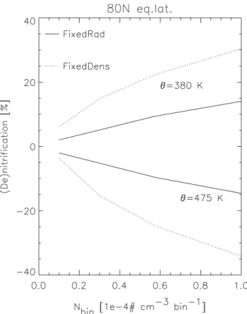
Fig. 9. De- and nitrification (%) on 20 January at 80◦N equiva-lent latitude, at 475 K and 380 K, respectively, using different total number densities (see Table 2) and both approaches; “FixedDens” (dotted line) and “FixedRad” (solid line).
of denitrification between an equilibrium and nonequilibrium approach were also found by Mann et al. (2002) for the same winter.
4.2.2 Total number density
The total number density of large particles (5–20 µm diame-ter) as observed by Fahey et al. (2001) was ∼2.3×10⁻⁴cm−3
on 20 January. The estimated uncertainty of this measure-ment is ±30% and may vary with the location inside the vortex. To test the model’s sensitivity to this parameter, the maximum allowable total number density was varied from 0.5 to 5×10⁻⁴cm−3, resulting in a nbin between 0.1 and
1×10⁻⁴cm−3 per size bin, respectively. The shape of the size distributions in terms of particle number concentrations are depicted in Fig. 3a, with the blue, black and red line denoting the contraints for the high, standard and low total number density runs, respectively.
Figure 9 shows the resulting (de)nitrification at 80◦N equivalent latitude against the total number density for these model runs on θ levels 380 K and 475 K, respectively. Even though the number density is variable within the “FixedRad” approach (i.e. nbinis merely used to define a threshold instead
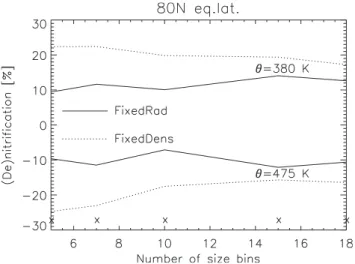
Fig. 10. De- and nitrification (%) on 20 January at 80◦N equivalent latitude, at 475 K and 380 K, respectively, using a different number of size bins (see Table 2) and both approaches. The crosses mark the number of size bins in the integrations that were done.
to this parameter, although less so than for the “FixedDens” approach. (De)nitrification increases with increasing nbin
due to an associated increase in the fraction of HNO3
par-titioned into NAT.
However, the maximum ¯d value becomes lower with in-creasing nbin (decreasing from 23.8 µm for 1×10⁻⁵cm−3
per bin to 18.2 µm for 1×10⁻⁴cm−3per bin at θ =430 K us-ing the “FixedDens” approach (not shown)), indicatus-ing that the growth of NAT particles is somewhat moderated by the choice of nbin. This is due to a related increase in
par-ticle mass (1mp ) in Eq. (2). This change is non-linear
with respect to nbin due to the increase in [NAT]tot. In all
cases, the [NAT]tot for the “FixedDens” method exceeded
that of the “FixedRad” approach by 30–40%. This increase in (de)nitrification with nbinwould eventually reach a
max-imal value due to the associated reduction in the available [HNO3(g)] within the vortex. The latter would result in a
limitation to particle growth, especially when a non-uniform HNO3(g)profile is considered. However, this situation would
only be reached when prescribing high number densities or during longer model runs. Moreover, temperature fluc-tuations would also limit the extent of the (de)nitrification by introducing periods where the evaporation of particles would hinder the sedimentation. Varying nbinfrom 0.25 to
1×10⁻⁴cm−3per bin, which is equivalent to halving or
dou-bling the total number density, leads to an increase in deni-trification from 12 to 34% at an equivalent latitude of 80◦N and θ =475 K for the “FixedDens” run, and from 5 to 15% for the “FixedRad” run (see Fig. 8).
4.2.3 The number of size bins
To make the algorithm as efficient as possible, it is impor-tant to know how many size bins (i.e. tracers) are required to
model denitrification. Figure 10 shows the (de)nitrification at 80◦N equivalent latitude calculated using an increasing
num-ber of size bins on identical θ levels as those shown in Fig. 8 for both model approaches. Due to the substantial increase in the redistribution of HNO3 with increasing particle number
density (see Sect. 4.2.2.), the total number density was kept constant throughout at 2.3×10⁻⁴cm−3, as prescribed in the base run. Since the size bin limits were not identical for each sensitivity run, the shape of the resulting size distributions varies depending on the number of bins used (c.f. Figs. 3a– d). However, it can be seen that the size spectrum essentially becomes flat once 7 or more bins are prescribed.
A pronounced result is that the methods are quite robust in calculated denitrification, since only small differences occur when the amount of size bins is doubled. The “FixedDens” approach results in more (de)nitrification than the “Fixe-dRad” approach regardless of the number of size bins used. But, remarkably, the differences in the vortex averaged val-ues between both approaches fall below 10% when the num-ber of size bins exceeds 7. “FixedRad” is less sensitive and only varies between 8 and 12% across the range of the cho-sen number of size bins, while the “FixedDens” denitrifica-tion clearly decreases with an increasing number of size bins, from 25% in the 5 bin simulation to 15% in the 18 bin run. This is due to the fact that the “FixedDens” particle growth is more sensitive to the resolution of the size spectrum (i.e. number of bins). The full content of the size bin is moved up or down during either growth or evaporation, while in the “FixedRad” approach the mass transport occurs only once the threshold nbinis exceeded. The use of more size bins,
with each of them a lower number density than the size bins in the standard run, results in a more concise and variable distribution of the mass over the size bins.
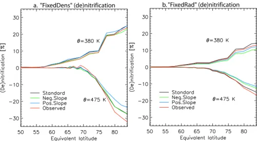
4.2.4 The shape of the size distribution
The particle size distributions measured by Fahey et al. (2001) suggest that constraining the model with a flat size distribution across the entire size spectrum maybe an over-simplification (as performed for the 7, 10, 15 and 18 bin sen-sitivity runs, c.f. Figs. 3b–d). To provide further insight into the extent to which the prescribed size spectrum has on the calculation of denitrification, we chose to alter the shape of the permitted size spectrum in a number of ways. For this purpose, we have performed runs with 7 bins using three distinctively different size distributions: one with decreas-ing and one with increasdecreas-ing nbinvalues from bin 2 to bin 7
(creating a negative and a positive “slope”, respectively) and one based on the distribution observed by Fahey et al. (2001). The shapes of these size distributions are shown in Figs. 3e–f and defined as the standard flat (black line), negative (blue), positive (green) and observed (red) distribution, respectively. Figures 11a and b show comparisons of the result-ing (de)nitrification at θ levels 380 and 475 K versus equivalent latitude for the “FixedDens” and “FixedRad”
a. "FixedDens" (de)nitrification b. "FixedRad" (de)nitrification
Fig. 11. De- and nitrification (%) along equivalent latitudes, at 475 K and 380 K, respectively, depending on the shape of the size distribution
(see Figs. 3e–3f). For (a) the “FixedDens” approach and (b) the “FixedRad” approach the number of size bins and total number density are fixed to seven and 2.3×10⁻⁴cm−3, respectively.
approaches, respectively. In summary it can be seen that the (de)nitrification changes by <8% for both approaches indicating that they are relatively robust with respect to the prescribed shape. For the run with the observed size spec-trum the model became unstable using the “FixedRad” ap-proach due to the last bin “overflowing” on the ninth day of the integration. However, the amount of NAT formed be-came rather excessive (>2 ppbv) in small regions of the vor-tex (not shown) meaning that no further discussion of this run is warranted. Prescribing an observed size distribution has the inherent weakness that the size distribution must re-main similar during the entire winter period. Unfortunately the size distributions shown in Northway et al. (2002b) indi-cate that the both the total number density and size distribu-tion change between 20 January and 3 February in the Arctic vortex for this winter. Therefore constraining the model with an observed size distribution would only be possible if many more measurements were available, during the whole winter, which is not feasible.
5 Discussion and conclusions
In this study we present an efficient and concise algorithm for the formation and sedimentation of NAT particles, which has been implemented in a global Eulerian 3D chemistry trans-port model using a non-equilibrium approach. For this pur-pose the transport of such particles is achieved by segregating the particles into distinct size bins, each of which is treated as an advected tracer. Two separate approaches were tested, one which prescribes a fixed particle number density per size bin (“FixedDens”) and the other which prescribes a fixed particle radius for each respective size bin (“FixedRad”). This algo-rithm has been applied in simulations over three selected
10-day periods during the Arctic winter 1999/2000, and the re-sulting particle sizes and number concentrations were found to agree favourably with those observed “in-situ” (Fahey et al., 2001; Brooks et al., 2003). Comparisons made with the results of a Lagrangian model study (Carslaw et al., 2002), from which the microphysical component of our algorithm was taken, reveals differences of between 0–4 µm for the di-ameters of the largest NAT particle formed, depending on the adopted approach (with the Eulerian model producing the larger sizes). Considering the differences in the perfor-mance and underlying concepts of both models we feel that agreement within ±20% is a satisfactory result. Although the results of the non-equilibrium approaches can only be tenta-tively compared with observations due to the restricted simu-lation periods, it is encouraging to find that the resulting den-itrification for such periods lies within the range of measured values (20–60%) for the Arctic winter 1999/2000 (Popp et al., 2001; Kleinb¨ohl et al., 2003; Santee et al., 2000). Clearly, further simulations are needed using realistic HNO3profiles,
with a full stratospheric chemistry scheme.
Substantial differences were found in both the magni-tude of denitrification and vertical/horizontal redistribution of HNO3, when compared against the results obtained using
a simple equilibrium approach. Applying the equilibrium ap-proach resulted in an unrealistically high removal of HNO3
when using an observed particle radius for 10–20 January. Decreasing the particle radius to 4 µm significantly reduced the HNO3removal, indicating the potential danger of using
such an approach. This large effect justifies the use of the computationally more expensive, but more realistic, treat-ment, of NAT particle growth and sedimentation. The re-sulting particle sizes of the “FixedDens” and the “FixedRad” method differ due to three main reasons: (i) particle size
discretization, (ii) treatment of NAT evaporation and (iii) di-lution of NAT mass by atmospheric mixing processes. When integrating over the selected 10-day periods this results in a difference in (de)nitrification between both methods of a fac-tor ∼2.]
The results from the sensitivity studies suggest that the model is rather robust and relatively insensitive to the ber of size bins used under conditions were the particle num-ber density summed over size bins remains constant. The “FixedRad” approach shows the smallest variation in deni-trification when changing the number of size bins, with the differences between both approaches becoming ≤10% for 10 size bins or more. This has advantages in that just a limited number of size bins (and thus tracers) are needed to account for nonequilibrium treatment of NAT and denitrification in a full chemistry run. Another important finding is that both ap-proaches are also quite insensitive to the shape of the size dis-tribution. However, both approaches show some sensitivity to the particle number density summed over size bins, with ∼17% increase in 10-day denitrification for the “FixedDens” method upon increasing the particle number density per size bin with 250% (from 0.4×10⁻⁵ to 1×10⁻⁴cm−3). Again, the “FixedRad” approach proved to be more robust towards this parameter, with the difference being lower at ∼7%. Here it should be noted that these sensitivity tests were performed during a prolonged period of low temperatures and therefore can be considered to be a worst case scenario. For many other periods temperature fluctations would lower the sensi-tivity of both methods to this parameter by introducing par-ticle evaporation. Considering the observed variability dur-ing 1999/2000,similar observations of the NAT total number density would be beneficial for future Arctic winters to re-move any bias introduced by using a prescribed value, as well as a continued effort in clarifying the details of the formation mechanisms of NAT. Our approaches do not require detailed knowledge on the shape of the size distribution, at least for the 1999/2000 winter.
For a more rigorous validation of our algorithms we are currently preparing simulations over the entire Arctic winter period of 1999/2000 with comprehensive chemistry active, as well as for more moderate Arctic winters. Lagrangian model studies have already shown that the nonequilibrium treatment of NAT calculates significant denitrification in other, more moderate winters (Mann et al., 2003). Using the Eulerian approaches presented here, we are now able to test the effect of denitrification during such a more moderate winter period to try and assess whether these differences lead to additional ozone depletion that warrants the increase in computational costs.
Acknowledgements. We would like to thank K. Carslaw, S. Davies,
G. Mann from the School of the Environment at the University of Leeds for their introduction to their nonequilibrium NAT algorithm and fruitful discussions. J. Buchholz, S. Meilinger and J. Lelieveld are also thanked kindly for their help and advice.
Edited by: B. K¨archer
References
Bregman, A., Lelieveld, J., van den Broek, M., Fischer, H., Sieg-mund, P., and Bujok, O.: The N2O and O2relationship for
mix-ing processes as represented by a three-dimensional chemistry-transport model, J. Geophys. Res., 105, 17 279–17 290, 2000. Bregman, A., Krol, M. C., Teyssedre, H., Norton, W. A., Iwi, A.,
Chipperfield, M., Pitari, G., Sundet, J. K., and Lelieveld, J.: Chemistry-Transport model comparison with ozone observations in the midlatitude lowermost stratosphere, J. Geophys. Res., 106, 17 479–17 496, 2001.
Bregman, A., Segers, A., Krol, M., Meijer, E., and van Velthoven, P.: On the use of mass-conserving wind fields in chemistry-transport models, Atm. Chem. Phys., 3, 447–457, 2003. Brooks, S. D., Baumgardner, D., Gandrud, B., Dye, J. E.,
North-way, M. J., Fahey, D. W., Paul Bui, T., Toon, O. B., and Tolbert, M. A.: Measurements of large stratospheric particles in the Arctic polar vortex, J. Geophys. Res., 108, D20, 4652, doi:10.1029/2002JD003278, 2003.
Carslaw, K. S., Kettleborough, J. A., Northway, M. J., Davies, S., Gao, R. S., Fahey, D. W., Baumgardner, D. G., Chipperfield, M. P., and Kleinb¨ohl, A.: A vortex-scale simulation of the growth and sedimentation of large nitric acid hydrate particles, J. Geo-phys. Res., 107, D20, 8300, doi:10.1029/2001JD000467, 2002. Chipperfield, M. P.: Multiannual simulations with a
three-dimensional chemical transport model, J. Geophys. Res., 104, 1781–1805, 1999.
Crutzen, P. and Arnold, F.: Nitric acid cloud formation in the cold Arctic stratosphere, a major cause for the springtime “‘ozone hole”, Nature, 324, 651–655, 1986.
Davies, S., Chipperfield, M. P., Carslaw, K. S., Sinnhuber, B.-M., Anderson, J. G., Stimpfle, R. M., Wilmouth, D. M., Fahey, D. W., Popp, P. J., Richard, E. C., von der Gathen, P., Jost, H., and Webster, C. R.: Modeling the effect of denitrification on Arctic ozone depletion during winter 1999/2000, J. Geophys. Res., 108, D5, 8322, doi:10.1029/2001JD000445, 2003.
Drdla, K., Schoeberl, M. R., and Browell, E. V.: Microphysical modelling of the 1999–2000 Arctic winter: 1. Polar stratospheric clouds, denitrification, and dehydration, J. Geophys. Res., 108, D5, 8312, doi:10.1029/2001JD000782, 2003.
Drdla, K., Turco, R. P., and Elliott, S.: Heterogeneous chemistry on Antarctic polar stratospheric clouds – a microphysical estimate of the extent of chemical processing, J. Geophys. Res., 98, D5, 8965–8981, 1993.
Fahey, D. W., Gao, R. S., Carslaw, K. S. et al.: The detection of large HNO3-containing particles in the winter Arctic Strato-sphere, Science, 1026–1031, 2001.
Fahey, D. W., Kelly, K. K., Kawa, S. R., Tuck, A. F., Loewenstein, M., Chan, K. R., and Heidt, L. E.: Observations of denitrification and dehydration in the winter polar stratospheres, Nature, 344, 321–324, 1990.
Fahey, D. W., Kelly, K. K., Ferry, G. V., Poole, L. R., Wilson, J. C., Murphy, D. M., Loewenstein, M., and Chan, K. R.: In situ measurements of total reactive nitrogen, total water and aerosol in a polar stratospheric cloud in the Antarctic, J. Geophys. Res., 94, 11 299–11 315, 1989.
Hanson, D. and Mauersberger, K.: Laboratory studies of the ni-tric acid trihydrate: Implications for the South polar stratosphere, Geophys. Res. Lett., 15, 855–858, 1988.
Jensen, E. J., Toon, O. B., Tabazadeh, A., and Drdla, K.: Impact of polar stratospheric cloud particle composition, number density, and lifetime on denitrification, J. Geophys. Res., 107, D20, 8284, doi:10.1029/2001JD000440, 2002.
Kleinb¨ohl, A., Bremer, H., von K¨onig, M., et al.: Vortexwide den-itrification of the Arctic polar stratosphere in winter 1999/2000 determined by remote observations, J. Geophys. Res., 108, D5, 8305, doi :10.1029/2001JD001042, 2003.
Knopf, D. A., Koop, T., Luo, B. P., Weers, U. G., and Peter, T.: Ho-mogeneous nucleation of NAD and NAT in liquid stratospheric aerosols: insufficient to explain denitrification, Atmos. Chem. Phys., 2, 207–214, 2002.
Koike, M., Kondo, Y., Takegawa, N. et al.: Redistribu-tion of reactive nitrogen in the Arctic lower stratosphere in the 1999/2000 winter, J. Geophys. Res., 107, D20, 8275, doi :10.1029/2001JD001089, 2002.
Krol, M. C., Lelieveld, J., Oram, D. E., Sturrock, G. A., Penkett, S. A., Brenninkmeier, C. A. M., Gros, V., Williams, J., and Scheeren, H. A.: Continuing emissions of methyl chloroform from Europe, Nature, 421, 131–135, 2003.
Krol, M.C., Houweling, S. Bregman, B., van den Broek, M., Segers, A., van Velthoven, P., Peters, W., Dentener, F., and Bergamaschi, P.: The two-way nested global chemistry-transport zoom model TM5: Algorithm and applications, Atmos. Chem. Phys. Discuss., 4, 3975–4018, 2004.
Mann, G. W., Davies, S., Carslaw, K. S., and Chipperfield, M. P.: Factors controlling Arctic denitrification in cold winters of the 1990s, Atmos. Chem. Phys., 3, 403–416, 2003.
Mann, G. W., Davies, S., Carslaw, K. S., and Chipperfield, M. P.: Polar vortex concentricity as a controlling factor in Arctic denitrification, J. Geophys. Res. 107, D22, 4663, doi:10.1029/20002JD002102, 2002.
Manney, G. L. and Sabutis, J. L.: Development of the polar vortex in the 1999–2000 Arctic winter stratosphere, Geophys. Res. Lett., 27, 2589–2592, 2000.
Northway, M. J., Gao, R. S., Popp, P. J., Holecek, J. C., Fahey, D. W., Carslaw, K. S., Tolbert, M. A., Lait, L. R., Dhaniyala, S., Flagan, R. C., Wennberg, P. O., Mahoney, M. J., Herman, R. L., Toon, G. C., and Bui, T. B.: An analysis of large HNO3 -containing particles sampled in the Arctic stratosphere during the winter of 1999/2000, J. Geophys. Res., 107, D20, 8298, doi:10.1029/2001JD001079, 2002a.
Northway, M. J., Popp, P. J., Gao, R. S., Fahey, D. W., Toon, G. C., and Bui, T. P.: Relating inferred HNO3flux values to the
dinitrification of the 1999–2000 Arctic Vortex, Geophys. Res. Lett., 29, D16, 1816, doi: 10.1029/2002GL015000, 2002b. Poole, L. R., Trepte, C. R., Harvey, V. L., Toon, G. C., and
Van-Valkenburg, R. L.: SAGE III observations of Arctic polar strato-spheric clouds – December 2002, Geophys. Res. Lett., 30, 23, 2216, doi :10.1029/2003GL018496, 2003.
Popp, P. J., Northway, M. J., Holecek, J. C., et al.: Lait, Severe and extensive denitrification in the 1999/2000 Arctic winter strato-sphere, Geophys. Res. Lett., 28, 2875–2878, 2001.
Prather, M. J.: Numerical advection by conservation of second-order moments, J. Geophys. Res., 91, 6671–6681, 1986. Rex, M., Salawitch, R. J., von der Gathen, P., Harris, N.
R. P., Chipperfield, M. P., and Naujokat, B.: Arctic ozone loss and climate change, Geophys. Res. Lett., 31, L04116, doi:10.1029/2003GL018844, 2004.
Rex, M., Harris, N. R. P., von der Gathen, P., et al.: Prolonged stratospheric ozone loss in the 1995–1996 winter, Nature, 389, 835–838, 1997.
Richard, E. C., Aikin, K. C., Andrews, A. E., et al.: Severe chemical ozone loss inside the Arctic polar vortex during win-ter 1999/2000 inferred from in situ airborne measurements, Geo-phys. Res. Lett., 28, 2197–2200, 2001.
Russell, G. L. and Lerner, J. A.: A new finite-differencing scheme for the tracer transport equation, J. Appl. Meteorol., 20, 1483– 1498, 1981.
Santee, M. L., Manney, G. L., Livesey, N. J., and Waters, J. W.: UARS Microwave Limb Sounder observations of denitrification and ozone loss in the 2000 Arctic late winter, Geophys. Res. Lett., 27, no. 19, 3213–3216, 2000.
Shine, K. P., Bourqui, M. S., de Forster, P. M., Hare, S. H. E., et al.: A comparison of model-simulated trends in stratospheric temper-atures, Quart. J. Met. Soc., 129, no. 590, 1565–1588, 2003. Sinnhuber, B.-M., Chipperfield, M. P., Davies, S., Burrows, J. P.,
Eichmann, K.-U., Weber, M., von der Gathen, P., Guirlet, M., Cahill, G. A., Lee, A. M., and Pyle, J. A.: Large loss of to-tal ozone during the Arctic winter of 1999/2000, Geophys. Res. Lett., 27, 21, 3473–3476, 2000.
Sugita, T., Kondo, Y., Nakajima, H., Schmidt, U., Engel, A., Oelhaf, H., Wetzel, G., Koike, M., and Newman, P. A.: Denitrification observed inside the Arctic vortex in February 1995, J. Geophys. Res., 103, 16 221–16 233, 1998.
Tabazadeh, A.: Commentary on “Homogeneous nucleation of NAD and NAT in liquid stratospheric aerosols : insufficient to explain denitrification” by Knopf et al., Atmos. Chem. Phys., 3, 863– 865, 2003.
Van den Broek, M. M. P., v. Aalst, M., Bregman, A., Krol, M., Lelieveld, J., Toon, G. C., Garcelon, S., Hansford, G. M., Jones, R. L., and Gardiner, T. D.: The impact of model grid zooming on tracer transport in the 1999/2000 Arctic polar vortex, Atmos. Phys. Chem., 3, 1833–1847, 2003.
Van den Broek, M. M. P., Bregman, A., and Lelieveld, J.: Model study of stratospheric chlorine activation and ozone loss dur-ing the 1996/1997 winter, J. Geophys. Res., 105, 28 961–28 977, 2000.
Waibel, A. E., Peter, Th., Carslaw, K. S., Oelhaf, H., Wetzel, G., Crutzen, P. J., P¨oschl, U., Tsias, A., Reimer, E., and Fischer, H.: Arctic ozone loss due to denitrification, Science, 283, 2064– 2069, 1999.