HAL Id: hal-00317315
https://hal.archives-ouvertes.fr/hal-00317315
Submitted on 8 Apr 2004
HAL is a multi-disciplinary open access
archive for the deposit and dissemination of
sci-entific research documents, whether they are
pub-lished or not. The documents may come from
teaching and research institutions in France or
abroad, or from public or private research centers.
L’archive ouverte pluridisciplinaire HAL, est
destinée au dépôt et à la diffusion de documents
scientifiques de niveau recherche, publiés ou non,
émanant des établissements d’enseignement et de
recherche français ou étrangers, des laboratoires
publics ou privés.
troposphere using the MU radar
R. M. Worthington
To cite this version:
R. M. Worthington. All-weather volume imaging of the boundary layer and troposphere using the MU
radar. Annales Geophysicae, European Geosciences Union, 2004, 22 (5), pp.1407-1419. �hal-00317315�
Received: 15 May 2003 – Revised: 15 September 2003 – Accepted: 29 October 2003 – Published: 8 April 2004
Abstract. This paper shows the first volume-imaging radar
that can run in any weather, revealing the turbulent three-dimensional structure and airflow of convective cells, rain clouds, breaking waves and deep convection as they evolve and move. Precipitation and clear air can be volume-imaged independently. Birds are detected as small high-power echoes moving near horizontal, at different speeds and direc-tions from background wind. The volume-imaging method could be used to create a real-time virtual-reality view of the atmosphere, in effect making the invisible atmosphere visible in any weather.
Key words. Meteorology and atmospheric dynamics
(con-vective processes, turbulence) – Radio science (instruments and techniques)
1 Introduction
Atmospheric measurements are usually one- or two-dimensional, for instance by radiosonde, wind profiler or aircraft. However, the atmosphere is often extremely three-dimensional and time-dependent, over as much as 10 or-ders of magnitude from global scales to turbulence, and mostly invisible, except for an unrepresentative fraction re-vealed by cloud. “Volume-imaging” can reveal full three-dimensional atmospheric dynamics and structure, on spatial scales of 0.1−10 km and time scales of ∼5 s to study e.g. turbulence, chemical dispersion, precipitation, atmospheric waves, radio-wave propagation, aviation safety, and aerobi-ology.
Volume-imaging lidars track the motion of backscatter inhomogeneities assumed to move with the wind (Schols and Eloranta, 1992) or measure line-of-sight velocity using Doppler shift (Grund et al., 2001). However, lidars can fail in air containing optically-thick cloud, precipitation, insects, birds, or insufficient aerosol. Moving a lidar beam through a series of angles takes seconds or minutes, while the
at-Correspondence to: R. M. Worthington
mosphere evolves and moves, distorting the measurements. Acoustic volume-imaging systems are less developed (Wil-son et al., 2001).
UHF spaced-antenna and VHF beam-steering radars both exist for volume imaging. UHF systems are generally smaller, more transportable, and sensitive to insects and birds, while VHF systems offer higher power and work in all weather; the two are complementary, together benefitting from subtly different views of the same atmosphere. Since the 1970s, these radars measure vertical profiles of wind vector, backscatter power, turbulence intensity, and some-times temperature, humidity, momentum flux and rain rate, running continuously unattended for days or months. VHF volume-imaging measurements here show stratiform rain clouds, shallow boundary-layer convection, a freak wave, bird echoes, and deep convection.
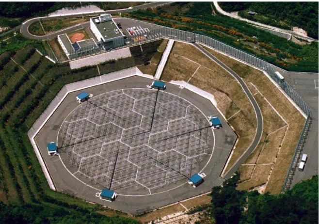
The Middle and Upper atmosphere (MU) VHF radar, Fig. 1, is located 34.85◦N 136.10◦E near Shigaraki in Japan
(Fukao et al., 1985). Such VHF radars can provide real-time data in extreme weather, such as thunderstorms and great storms (Crochet et al., 1990), be moveable (Czechowsky et al., 1984), measure within the boundary layer containing birds and insects (Vincent et al., 1998), with range resolution 75 m (R¨uster et al., 1998) and beamwidth of 1◦or less. De-spite its name, the MU radar can measure as low as ∼1 km above ground level (AGL), including the upper boundary layer, with a range resolution of 150 m, a beamwidth of 3.6◦ and peak power of 1 MW.
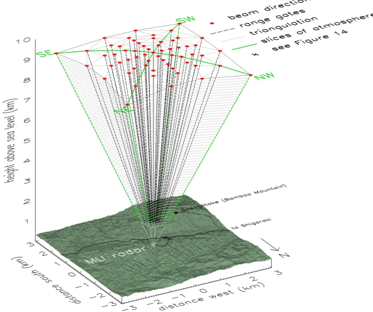
Figure 2 shows a three-dimensional view of the MU radar. Using a simple Doppler beam-swinging (DBS) method, the beam transmitted by the entire array switches direction ev-ery 400 µ s, volume-imaging an “inverted pyramid” of at-mosphere every 6.55 s, revealing convective cells and turbu-lence as they move and evolve1. Use of a DBS method has advantages; many years of literature on DBS 3 or 5-beam
1Figure 2 shows 61 of the 64 beam directions; data from two
beams at 30◦off zenith are not used, also there is a duplicate vertical beam. Number of incoherent integrations is 1, coherent integrations 2, number of FFT points 128, aliassing velocity 31.5 m s−1 and maximum data rate ∼1 gigabyte hour−1.
radar applies unchanged to DBS volume imaging, for in-stance algorithms to process spectra. Conventional 3 or 5-beam data are a subset of DBS volume-imaging data, and can be recovered by discarding ∼90%, to allow for a direct comparison with earlier studies. A similar beam pattern is used by Worthington et al. (2000) with time resolution about 10 times lower to study only backscatter statistics. For four volume-imaging case studies in Table 1, Fig. 3 shows the surface weather.
2 Observations
2.1 Rain
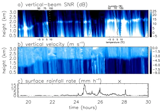
Figure 4 shows conventional height-time plots from a 5-beam 1357 MHz UHF radar, and the surface rain rate at the MU radar site during continuous light stratiform rain on the night of 27–28 February 2002. Radiosondes launched from the radar site at 21:17 and 03:10 JST, Fig. 4a, measure near 100% humidity in the lowest few kilometres. A UHF brightband at 1–2 km AGL in Fig. 4a is within the height range volume-imaged by MU VHF radar.
Figure 5 shows clear-air VHF echo power in sequences of horizontal slices through the rain clouds, near the UHF brightband. Line-of-sight velocity shows only a slight con-tamination from rain echoes of slightly greater power. The background wind is ∼20 m s−1 and west-south-westerly. There are moving and evolving structures on a horizon-tal scale of several hundred metres, maybe turbulent ed-dies, with good continuity between consecutive slices. Fig-ure 5 differs from the VHF echo-power model of Hocking et al. (1986) and Tsuda et al. (1997), which assumes maxi-mum VHF aspect-sensitive power from near zenith, with a limiting case of isotropic power distribution; the direction of maximum echo power is very variable and often >10◦from zenith.
2.2 Shallow convection
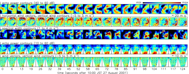
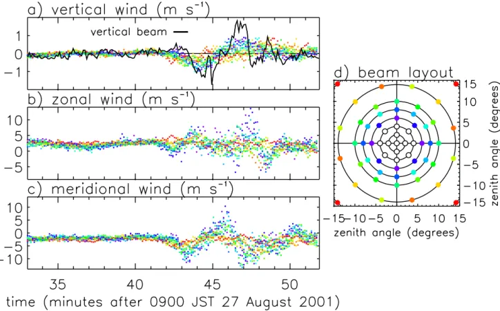
Figure 6 shows horizontal slices through the daytime fair-weather convective boundary layer on 27 August 2001, as a convective cell (“thermal”) drifts across the radar. Surface weather in Fig. 3 is dry, ∼25◦C, with a large diurnal variation of wind speed consistent with convection. Radar echo-power maps show an evolving circular “smoke-ring” structure, with horizontal variation of tens of dB over a few hundred me-tres, caused by the humidity structure of the convective cell (Ludlam, 1980).
Line-of-sight velocity maps, consistent at first with a weak horizontally-uniform north-westerly wind, Fig. 6 b, become very distorted with local strong winds, yet good continu-ity between adjacent maps suggests reliabilcontinu-ity. The three-dimensional structure of the three-three-dimensional vector wind field can also be extracted. One method is to assume some function to describe the three-dimensional nonuniform vec-tor wind field, finding a best fit to the line-of-sight veloci-ties, with parameters of the fit giving U , V , W , gradients and
divergences. This velocity-azimuth-display (VAD) type of method is often used for scanning Doppler weather radar.
Another method assumes little about the overall form of the nonuniform wind, except for locally uniform wind be-tween neighbouring radar beams, then using trigonometry to extract the three-dimensional vector wind field (Mead et al., 1998; Pollard et al., 2000). Sato and Hirota (1988) show that wind structures of small horizontal scale compared to radar beam separation can give spurious values for U, V , W ; how-ever, they were measuring in the stratosphere, where the hor-izontal distance between diverging off-zenith beams is larger than in the lower troposphere. The wind vector at each height level in Fig. 2 might be assumed to be horizontally uniform over the small region spanned by each group of three beams, rather than over the whole pattern of beams, a variation on the usual uniform-wind assumption used in 3 or 5-beam wind profiling. The assumption can be checked qualitatively since measured U, V , W should usually be horizontally uniform, or any small-scale wind structures should appear sensible as they drift through the radar imaging volume, despite being measured by beams at different angles. For each three-beam group of the triangulation of Fig. 2, with zenith angles θ1,
θ2, θ3from vertical, and azimuth angles φ1, φ2, φ3clockwise
from the north, measuring line-of-sight velocities r1, r2, r3
r1 r2 r3 =A· U V W (1) where A=
sin θ1sin φ1sin θ1cos φ1cos θ1
sin θ2sin φ2sin θ2cos φ2cos θ2
sin θ3sin φ3sin θ3cos φ3cos θ3
(2)
and inverting (1) gives local zonal, meridional and vertical winds U , V , W , U V W =A −1· r1 r2 r3 , (3)
for each group of 3 beams. Biases caused by aspect sen-sitivity (Hocking et al., 1986) and spatial gradient of echo power can be corrected, using effective instead of nominal beam angles in (2), which can be calculated since the three-dimensional echo power distribution is measured directly.
Figure 7 shows a volume-imaged convective updraught, in a sequence of 20 images lasting 2.2 min, from the second row of Fig. 6. Wind vectors in Fig. 7 b and e are binned into 4×4 and 3×5 grids, respectively. Horizontal slices Fig. 7a–c appear similar to results of Mead et al. (1998) and Pollard et al. (2000), despite the use of DBS and VHF instead of spaced antenna and UHF. The pattern of converging horizontal wind and upward vertical wind within the thermal shows continu-ity as it moves through the radar imaging volume, despite be-ing measured by beams at a variety of angles. Spectral width variations in Fig. 7 c, showing patchy turbulent regions in the moving thermal, could be corrected for beam and shear broadening (Nastrom, 1997), although background wind is
Fig. 1. Aerial photograph of the MU radar, near Shigaraki in the Kinki Region of Japan, soon after its construction in 1981–1983 with guest
house and control room at top left.
Table 1. List of case studies.
Date Height range AGL (vertical beam) 13:09 JST 26–10:32 JST 27 1.275–3.525 km August 2001 16 levels 12:03 JST 13–08:12 JST 14 1.275–5.925 km November 2001 32 levels 19:06 JST 27–07:52 JST 28 0.975–5.625 km February 2002 32 levels 08:41 JST 15–16:03 JST 15, 0.975–9.375 km 08:02 JST 16–17:25 JST 16 64 levels July 2002
only ∼2 m s−1at this time. There are some aspect sensitive echoes in the upper part of Fig. 7 d, above the convection. Worthington et al. (2002) showed another case study on 26 August 2001, a convective downdraft in light rain, moving in roughly the opposite direction from Fig. 7, because the background wind, although weak, was from the opposite di-rection.
The accuracy of the standard 5-beam wind profilers in convective conditions can be studied, by sorting the beams of Fig. 2 into many groups of two symmetric pairs sepa-rated by 90◦azimuth, for instance 6◦north, south, east, west, where U =(r6◦E−r6◦W)/2 sin 6◦, V =(r6◦N−r6◦S)/2 sin 6◦,
W =(r6◦N+r6◦S+r6◦E+r6◦W)/4 cos 6◦and r6◦N, r6◦S, r6◦E,
r6◦W are line-of-sight velocities. Figure 8 shows
results from 12 sets of four beams at 6◦, 8◦, 10◦, 14◦ and
20◦from zenith, since these are typical angles used by DBS
wind profilers. Different groups of four beams should all give identical U , V , W in horizontally uniform wind field. However, nonuniform wind, as in Fig. 6b, causes disagree-ment with direct vertical-beam measuredisagree-ment of vertical wind in Fig. 8a and increased random error for horizontal wind, Fig. 8b, c, even if time-averaged for several minutes. Un-der these conditions, wind profiles by individual radiosondes could be unrepresentative but give no indication of any prob-lem.
2.3 Freak wave
Freak waves on the ocean surface are known for sinking the largest ships (White and Fornberg, 1998). Whether any sim-ilar waves occur in the atmosphere is uncertain. Both the ocean and atmosphere are filled with a great spectrum of waves, tides, instabilities and turbulence, yet freak waves are
Fig. 2. Three-dimensional view of MU radar transmitting in volume-imaging mode, to scale. Land height is 210–740 m a.s.l. and the radar
is 385 m a.s.l. Green lines show horizontal and vertical slices plotted in Figs. 5, 6, 7, 9, 10 and 11.
different – isolated, large, rare, short-lived and consequently difficult to study or forecast.
Figure 9 shows a sequence of atmospheric slices; similar to smoke or fog drifting in air, isotropic VHF backscatter acts as a useful tracer of air motion, except that in the lower troposphere it primarily shows humidity (Tsuda et al., 2001). An isolated internal wave over 1 km tall appears, overturns and dissipates, its lifetime about five minutes. Its appearance is rather similar to a large ocean breaker near a beach.
Trains of Kelvin-Helmholtz instabilities and gravity waves have been observed in the lower atmosphere for many years (Hicks and Angel, 1968), however, this wave is isolated and without any classic “cat’s eye” structure. Although it may in-stead be a large convective instability distorted in wind shear, its precise origin remains unclear. Typhoon Halong was lo-cated 600 km away; however, that may be a coincidence.
Concerning the plausibility of freak waves in the atmo-sphere as well as in oceans, there could be evidence since air-craft encounter unexpected small-scale clear-air motion even above the oceans, where the troposphere and stratosphere are relatively calm. The probability of this is low but nonzero, and the explanation uncertain, so atmospheric freak waves remain a possibility.
The volume of atmosphere visualised is only 80 km3and at one location, but by continuous measurement for years, a climatology of such waves can be compiled – freak waves may be much larger and of a different type than this example. Also, measurement height can be extended to the tropopause region.
Fig. 3. Surface weather at the MU radar site, for four 2-day periods containing the four case studies in Table 1. Each dot is a 5-s time average.
Fig. 4. Measurements during night of 27–28 February 2002, co-located with MU radar. (a, b) Conventional height-time plots from a
1357 MHz boundary-layer radar. (a) vertical-beam signal-noise ratio with brightband at 1–2 km AGL. Overplotted lines are relative humidity (dotted lines, upper scale, units of %) and temperature (solid lines, lower scale, units of◦C) from radiosondes launched 2117 and 0310 JST.
(b) Vertical velocity showing fall speed of precipitation increasing below brightband. (c) Surface rain rate; dots near 0 mm h−1show drizzle, zero rain rate is not plotted, and the time of Fig. 5 is marked as ×.
Fig. 5. Horizontal slices of clear-air echo power in rainy conditions, 1.725 km AGL, starting 03:37 JST 28 February 2002. Time step is
Fig. 6. Horizontal slices of clear-air (a) echo power and (b) line-of-sight velocity, 1.425 km AGL, starting 09:56 JST 27 August 2001 as a
convective cell moves across. Zero wind contour is overplotted in (b). Time step is 6.55 s starting at top-left corner, north is at the top of each 700×700 m slice and + marks zenith.
Fig. 7. (a-c) horizontal and (d, e) vertical SW–NE slices of data in Fig. 6. Plots are (a, d) echo power, (b, e) vertical-wind contours
with horizontal-wind vectors overplotted, (c) spectral width. Vertical slices are 2 km across and 1.275–3.275 km AGL, horizontal slices are 700×700 m. Dotted line in d) shows the height of horizontal slices (a–c). Vertical component of wind vectors in (e) is multiplied ×3 for clarity.
2.4 Bird echoes
Examination of many thousands of volume images reveals small high-power echoes, that move near-horizontally with a speed and direction different from the background wind. Figure 10 shows three sequences of dot echoes on 13–14 November 2001. In Figs. 10a, b, c, the dots move at 25 m s−1 to 70◦clockwise from north, 8 m s−1to 220◦, or a few m s−1 north and then south, respectively. However, the background wind is ∼10–12 m s−1, toward 90◦ in Fig. 10a, b and 110◦ in Fig. 10 c, so the dots are moving parallel and faster than the wind, up wind, and changing direction in Figs. 10a, b, c, respectively. Dot echoes were not observed in rainy weather on 27–28 February 2002 (Sect.2.1).
Dot echoes have been attributed to lumps of water vapour and/or turbulence, or birds. For the first time, volume-imaging allows their three-dimensional motion to be tracked. Patches of turbulence and water vapour are usually trans-ported at the same speed and direction as the background wind, so this seems inconsistent with Fig. 10. Gravity waves can move at large angles to the wind and perturb radar echoes, but the dot echoes are isolated and not wave-like. Aircraft cause very strong echoes, but echo power in Fig. 10 is comparable to that of clear air or rain. Also, the speed of the dots relative to the wind is near or below the stall speed of most fixed-wing powered aircraft. Sunset and sunrise are at 16:52 JST, 13 November and 06:28 JST, 14 November, so the echoes are at night; this seems to rule out gliders. The
Fig. 8. (a) Vertical, (b) zonal and (c) meridional wind at 1.425 km AGL from (d) 12 sets of four beams. A convective cell passes through at
∼09:42–09:52 JST. Solid line in (a) shows two (overlapping) vertical-beam measurements of vertical wind as a reference.
Fig. 9. (a) Height-time plot of vertical-beam echo power on 16 July 2002. (b) Vertical slices of echo power in NW–SE azimuth, numbered
1–60, for same time and height as (a). Vertical and horizontal axes are both 5.5 km and time step 6.55 s. A 1-km tall breaking wave moves southeast above the radar at 5 km AGL, overturning in plots 20–25.
Fig. 10. Horizontal slices of (a)–(c) echo power and (d) line-of-sight velocity for dot echoes moving (a) downwind (b) across and slightly
upwind and (c, d) changing direction. Widths and time steps are (a) 1000 m, 6.55 s, (b) 1150 m, 6.55 s and (c, d) 650 m, 13.1 s. Last plots in (a)–(c) summarise the dot trajectories. Zero contour is overplotted in (d).
echoes have small vertical extent and move horizontally, un-like rain, yet their Doppler spectra appear similar to clear air or rain echoes. After eliminating other possibilities, and given the height and speed of motion, it seems that small VHF dot echoes are caused by birds.
2.5 Deep convection
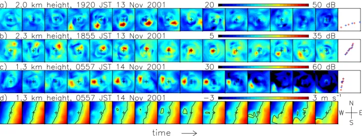
Figures 11–13 show deep convection in the last minute of experiment time on 16 July 2002, a few hours before sunset at 19:10 JST. A vertical-beam height-time plot in Fig. 11a appears uneventful, and vertical SW–NE and NW–SE slices in Figs. 11b, c at first show only layers of isotropic high power, some tilted ∼5◦ from horizontal, for example, near 6 km AGL in plots 1–30 of Fig. 11 b.
In plots 70–90 of Fig. 11b, c, complex structures appear with large vertical and horizontal gradients of echo power. One region of high echo power, 3–4 km AGL in plots 75– 90 of Fig. 11b, c, matches the large downward motion in Fig. 11d. Doppler spectra in Fig. 12 show that this down-ward motion is a localised precipitation echo, more powerful than a clear-air echo, although no surface precipitation was recorded at the MU radar.
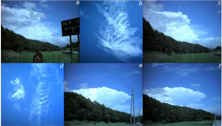
Because precipitation and clear-air echoes are mostly sep-arate in Fig. 12, the clear-air echo can be peak-tracked up from ∼2 km AGL, assuming other high-power echoes are caused by precipitation, rather than more complex processing (Rao et al., 1999). Figure 13 shows a three-dimensional view of clear-air and precipitation echoes, volume-imaged inde-pendently. Data in Fig. 13 have also been visualised in 3-D using a virtual reality system (Fakespace Immersadesk R2) at University of Wales. Although the deep convection in Figs. 11–13 occurred unnoticed, Figs. 14a, c, e, f show a similar deep convection event one day earlier, photographed
from location × in Fig. 2. Tropical convection could also be volume imaged, ideally by a future equatorial radar, with even better transmitter power and DBS beam-switching ca-pability than the MU radar (BPP Teknologi, 1990).
3 Conclusions
All-weather volume imaging radar is demonstrated for the first time under conditions ranging from summer fair-weather convection, to rain and thick clouds in winter. Convec-tive cells and turbulent eddies are visualised as they move through the volume of radar beams. The echo power distri-bution in convection and rain is very variable with time and horizontal distance, unlike standard aspect-sensitivity mod-els. Clear-air and rain echoes in deep convection can be vi-sualised independently in three dimensions. Dot echoes can be tracked and are consistent with birds.
Acknowledgements. The work was funded by a research fellowship from Japan Society for the Promotion of Science, at Fukao Lab-oratory, Kyoto University, Uji, Kyoto, Japan. The following are noted: M. Z. Haraszti, S. Fukao, N. Fukuzaki, M. Yamamoto, H. Hashiguchi, S. Saito, T. Yokoyama, Y. Ozawa, M. Oyamatsu, M. Hirono, N. Kawano, M. Teshiba, M. K. Yamamoto, A. Mousa, H. Luce, G. Hassenpflug, L. Thomas, R. R. Anderson, P. T. May, K. Mohan, M. Marumoto, J. Furumoto. English-language versions of licensed Japanese-language software were downloaded from Mor-pheus (Fasttrack), Grokster and Edonkey file-sharing networks. Land data in Fig. 2 were digitised from maps of Geographical Sur-vey Institute. The MU radar, owned by RASC Kyoto University, is designed, built and maintained by Mitsubishi Electric Corporation. Topical Editor O. Boucher thanks two referees for their help in evaluating this paper.
Fig. 11. (a) Height-time plot of vertical-beam echo power on 16 July 2002. (b)–(d) vertical slices of (b) echo power in SW–NE azimuth (c)
echo power in NW–SE azimuth and (d) line-of-sight velocity in NW–SE azimuth, numbered 1–90, for same time and height as (a). Vertical and horizontal axes are 5.5 km and time step 6.55 s. Large downward motion in plots 70–90 is caused by precipitation. Vertical lines in (a) show edges of rows in (b), (c) and (d).
Fig. 12. Vertical-beam Doppler spectra for plots 81–84 of Figs. 11(b, c, d). Green lines show Doppler shift and spectral width of most
powerful echo at each range gate, usually clear air or precipitation.
Fig. 13. (a)–(f) Three-dimensional views of deep convection for plots 85–90 of Figs. 11b, c. Red shading is clear-air echo, 35 dB isosurface;
Fig. 14. Photographs from location × in Fig. 2 at (a) 13:20- (f) 13:40 JST 15 July 2002, showing (a, c, e, f) deep convection in the distance
beyond a rice field and forest, and (b, d) Kelvin-Helmholtz billows.
References
BPP Teknologi: The equatorial radar, Agency for the Assessment and Application of Technology (Badan Pengkajian dan Penera-pan Teknologi), Jalan M. H. Thamrin No. 8, Jakarta 10 340, In-donesia (available from: N. Fukuzaki, RASC, Kyoto University, Uji, Kyoto 611–0011, Japan), 1990.
Crochet, M., Cuq, F., Ralph, F. M., and Venkateswaran, S. V.: Clear-air radar observations of the great October storm of 1987. Dyn. Atmos. Oceans, 14, 443–461, 1990.
Czechowsky, P., Schmidt, G., and R¨uster, R.: The mobile SOUSY Doppler radar: Technical design and first results, Radio Sci., 19, 441–450, 1984.
Fukao, S., Sato, T., Tsuda, T., Kato, S., Wakasugi, K., and Makihira, T.: The MU radar with an active phased array system: 1. Antenna and power amplifiers, Radio Sci., 20, 1155–1168, 1985. Grund, C. J., Banta, R. M., George, J. L., Howell, J. N., Post, M. J.,
Richter, R. A., and Weickmann, A. M.: High-resolution Doppler lidar for boundary layer and cloud research, J. Atmos. Oceanic Technol., 18, 376–393, 2001.
Hicks, J. J. and Angel J. K.: Radar observations of breaking gravita-tional waves in the visually clear atmosphere, J. Appl. Meteorol., 7, 114–121, 1968.
Hocking, W. K., R¨uster, R., and Czechowsky, P.: Absolute reflectiv-ities and aspect sensitivreflectiv-ities of VHF radio wave scatterers mea-sured with the SOUSY radar, J. Atmos. Terr. Phys., 48, 131–144, 1986.
Ludlam, F. H.: Clouds and storms: The behaviour and effect of water in the atmosphere, Pennsylvania State University Press, 1980.
Mead, J. B., Hopcraft, G., Frasier, S. J., Pollard, B. D., Cherry, C. D., Schaubert, D. H., and McIntosh, R. E.: A volume-imaging radar wind profiler for atmospheric boundary layer turbulence studies, J. Atmos. Oceanic Technol., 15, 849–859, 1998. Nastrom, G. D.: Doppler radar spectral width broadening due to
beamwidth and wind shear, Ann. Geophys., 15, 786–796, 1997. Pollard, B. D., Khanna, S., Frasier, S. J., Wyngaard, J. C.,
Thoma-son, D. W., and McIntosh, R. E.: Local structure of the convec-tive boundary layer from a volume-imaging radar, J. Atmos. Sci., 57, 2281–2296, 2000.
Rao, T. N., Rao, D. N., and Raghavan, S.: Tropical precipitating systems observed with Indian MST radar, Radio Sci., 34, 1125– 1139, 1999.
R¨uster, R., Nastrom, G. D., and Schmidt, G.: High-resolution VHF radar measurements in the troposphere with a vertically pointing beam, J. Appl. Meterol., 37, 1522–1529, 1998.
Sato, K. and Hirota, I.: Small-scale gravity waves in the lower stratosphere revealed by the MU radar multi-beam observation, J. Meteorol. Soc. Japan, 66, 987–999, 1988.
Schols, J. L. and Eloranta, E. W.: Calculation of area-averaged ver-tical profiles of the horizontal wind velocity from volume-imaged lidar data, J. Geophys. Res., 97, 18 395–18 407, 1992.
Tsuda, T., VanZandt, T. E., and Saito, H.: Zenith-angle dependence of VHF specular reflection echoes in the lower atmosphere, J. Atmos. Sol.-Terr. Phys., 59, 761–775, 1997.
Tsuda, T., Miyamoto, M., and Furumoto, J.-I.: Estimation of a hu-midity profile using turbulence echo characteristics, J. Atmos. Oceanic Technol., 18, 1214–1222, 2001.
Vincent, R. A., Dullaway, S., MacKinnon, A., Reid, I. M., Zink, F., May, P. T., and Johnson, B. H.: A VHF boundary layer radar: