Ten-year global distribution of downwelling longwave radiation

HAL Id: hal-00295388

https://hal.archives-ouvertes.fr/hal-00295388

Submitted on 30 Jan 2004

HAL is a multi-disciplinary open access

archive for the deposit and dissemination of

sci-entific research documents, whether they are

pub-lished or not. The documents may come from

teaching and research institutions in France or

abroad, or from public or private research centers.

L’archive ouverte pluridisciplinaire HAL, est

destinée au dépôt et à la diffusion de documents

scientifiques de niveau recherche, publiés ou non,

émanant des établissements d’enseignement et de

recherche français ou étrangers, des laboratoires

publics ou privés.

radiation

K. G. Pavlakis, D. Hatzidimitriou, C. Matsoukas, E. Drakakis, N.

Hatzianastassiou, I. Vardavas

To cite this version:

K. G. Pavlakis, D. Hatzidimitriou, C. Matsoukas, E. Drakakis, N. Hatzianastassiou, et al.. Ten-year

global distribution of downwelling longwave radiation. Atmospheric Chemistry and Physics, European

Geosciences Union, 2004, 4 (1), pp.127-142. �hal-00295388�

www.atmos-chem-phys.org/acp/4/127/

SRef-ID: 1680-7324/acp/2004-4-127

Chemistry

and Physics

Ten-year global distribution of downwelling longwave radiation

1_{Foundation for Research and Technology-Hellas, Heraklion, Crete, Greece} 2_{Department of Physics, University of Crete, Heraklion, Crete, Greece}

3_{Department of Electrical Engineering, Technological Educational Institute of Crete, Greece} 4_{Department of Physics, University of Ioannina, Greece}

Received: 26 July 2003 – Published in Atmos. Chem. Phys. Discuss.: 13 October 2003 Revised: 18 December 2003 – Accepted: 15 January 2004 – Published: 30 January 2004

Abstract. Downwelling longwave fluxes, DLFs, have been

derived for each month over a ten year period (1984–1993), on a global scale with a spatial resolution of 2.5×2.5 de-grees and a monthly temporal resolution. The fluxes were computed using a deterministic model for atmospheric ra-diation transfer, along with satellite and reanalysis data for the key atmospheric input parameters, i.e. cloud proper-ties, and specific humidity and temperature profiles. The cloud climatologies were taken from the latest released and improved International Satellite Climatology Project D2 se-ries. Specific humidity and temperature vertical profiles were taken from three different reanalysis datasets; NCEP/NCAR, GEOS, and ECMWF (acronyms explained in main text). DLFs were computed for each reanalysis dataset, with dif-ferences reaching values as high as 30 Wm−2_{in specific}

re-gions, particularly over high altitude areas and deserts. How-ever, globally, the agreement is good, with the rms of the difference between the DLFs derived from the different re-analysis datasets ranging from 5 to 7 Wm−2. The results are presented as geographical distributions and as time series of hemispheric and global averages. The DLF time series based on the different reanalysis datasets show similar seasonal and inter-annual variations, and similar anomalies related to the 86/87 El Ni˜no and 89/90 La Ni˜na events. The global ten-year average of the DLF was found to be between 342.2 Wm−2 and 344.3 Wm−2, depending on the dataset. We also con-ducted a detailed sensitivity analysis of the calculated DLFs to the key input data. Plots are given that can be used to obtain a quick assessment of the sensitivity of the DLF to each of the three key climatic quantities, for specific climatic conditions corresponding to different regions of the globe. Our model downwelling fluxes are validated against avail-able data from ground-based stations distributed over the globe, as given by the Baseline Surface Radiation Network.

Correspondence to: I. Vardavas

(vardavas@iesl.forth.gr)

There is a negative bias of the model fluxes when compared against BSRN fluxes, ranging from −7 to −9 Wm−2_{, mostly}

caused by low cloud amount differences between the station and satellite measurements, particularly in cold climates. Fi-nally, we compare our model results with those of other de-terministic models and general circulation models.

1 Introduction

The estimation of the surface radiation budget represents a major objective of the World Climate Research Programme as demonstrated by its Global Energy and Water Cycle Ex-periment (GEWEX), and in particular the GEWEX Surface Radiation Budget Project (Stackhouse et al., 1999; Gupta et al., 1999). The amount of downwelling longwave radia-tion reaching the surface of the Earth is an indicator of the strength of the atmospheric greenhouse effect and hence it is a key parameter in climate modelling. The only reliable direct measurements of downwelling longwave fluxes at the surface are those provided by well-calibrated surface instru-ments. Current archives of such measurements have a very limited temporal and geographical coverage. For example, downwelling longwave fluxes (DLF) reaching the surface, exist for about 36 BSRN (Baseline of Surface Radiation Net-work) stations around the world and in most cases data exist only since the mid-nineties. Therefore, in order to monitor the surface downwelling longwave radiation on a global scale and over a long enough period to identify climate change impacts, one needs to rely on satellite data, in conjunction with radiative transfer models, with validation against sur-face measurements.

The reliability of the computed fluxes is primarily affected by its sensitivity to cloud cover and cloud properties, and to the vertical profiles of temperature and humidity, especially in the lower troposphere. Clouds, which are a very impor-tant determinant of the surface radiation budget, represent a

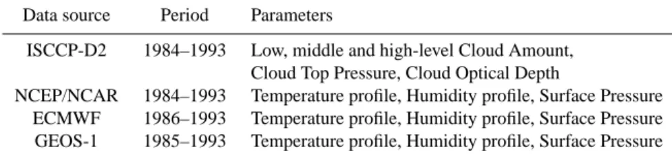
Table 1. List of the meteorological data sources used as inputs to the radiation code.

Data source Period Parameters

ISCCP-D2 1984–1993 Low, middle and high-level Cloud Amount, Cloud Top Pressure, Cloud Optical Depth

NCEP/NCAR 1984–1993 Temperature profile, Humidity profile, Surface Pressure ECMWF 1986–1993 Temperature profile, Humidity profile, Surface Pressure GEOS-1 1985–1993 Temperature profile, Humidity profile, Surface Pressure

major uncertainty in climate modelling (Intergovernmental Panel on Climate Change, IPCC 2001). The International Satellite Cloud Climatology Project (Rossow and Schiffer, 1991; 1999), which is also part of the WCRP GEWEX Project, provides one of the most extensive and comprehen-sive global cloud climatologies currently available, as well as Earth surface and atmospheric parameters. The latest re-leased D-series cloud datasets cover a sixteen-year period (July 1983 to December 2000) and show significant improve-ments over the earlier C-series, e.g. increased sensitivity of low-cloud detection, especially at high latitudes and over snow or ice in polar regions, as well as increased cirrus cloud detection over land. The changes in the detection thresholds for the D-series analysis have been successful in reducing the main biases of the C-series results found in validation ies (see Rossow and Schiffer, 1999, for details). All stud-ies of the Earth’s radiation field, based on ISCCP data that have been published to date have relied on C-series cloud climatology (Darnell et al., 1992; Schweiger and Key, 1994; Rossow and Zhang, 1995; Fowler and Randall, 1996; Chen and Roeckner, 1996; Yu et al., 1999; Gupta et al., 1999; Hatzianastassiou et al., 1999; 2001a; 2001b; Hatzianastas-siou and Vardavas, 2001). They also have limitations in tem-poral and/or spatial coverage, spatial resolution, and valida-tion with surface measurements.

The purpose of the present paper is to provide a fully validated dataset of monthly averaged DLF at the surface of the Earth, for the entire globe, on a 2.5-degree reso-lution (equal-angle), for 10 years (1984–1993), based on ISCCP-D2 cloud data. The fluxes are available on the web http://esrb.iesl.forth.gr/LW-Fluxes. They are computed by a radiation transfer model, which is based on a detailed radiative-convective code (see Sect. 2 for details). Temper-ature and humidity profiles from three different reanalyses (NCEP/NCAR, ECMWF and GEOS) are used and the cor-responding DLF results are inter-compared, following the recommendation of Kistler et al. (2001) regarding the use of reanalysis data for long-term climate studies. The calcu-lated fluxes are compared with surface measurements from the Baseline Surface Radiation Network (BSRN) (Ohmura et al., 1998).

2 Model and input data

2.1 Model description

In a series of previous papers, we have presented calculations of the longwave radiation budget for 10◦ latitudinal zones for the Northern (Hatzianastassiou et al., 1999) and South-ern Hemisphere (Hatzianastassiou and Vardavas, 2001), and for the polar regions (Hatzianastassiou et al., 2001a), based on a radiation transfer model, which is a simplification of a detailed radiative-convective code developed for climate change studies (Vardavas and Carver, 1984). Here, we use the same code, but modified to derive fluxes on a 2.5-degree spatial resolution and monthly temporal resolution, for both hemispheres. We use simple expressions for the total absorp-tion of infrared radiaabsorp-tion by the atmospheric molecules, in-dependently in each 2.5◦×2.5◦grid-box, dividing vertically the atmosphere (from the surface up to 50 mb) in about 5 mb layers to ensure that they are optically thin with respect to the Planck mean longwave opacity, and using simple trans-mission coefficients which depend on the amount of absorb-ing molecules in each layer. The molecules considered are; H2O, CO2, CH4, O3, and N2O. The sky is divided into clear

and cloudy fractions. The cloudy fraction includes three non-overlapping layers of low, middle and high-level clouds, however the effect of cloud overlap on the model results is examined using two different schemes in Sect. 5. Expres-sions for the fluxes for clear and cloudy sky can be found in Hatzianastassiou et al. (1999).

2.2 Input data

All of the cloud meteorological data except for the cloud-base temperature are taken from the ISCCP-D2 data set, which supplies monthly means for 72 meteorological vari-ables in 2.5-degree equal-angle grid-boxes. More specifi-cally, the variables used include: the cloud cover fractions for low, middle, and high-level clouds, the corresponding cloud top pressures and temperatures, and the cloud optical depth, which is particularly relevant for the high clouds, since low and middle clouds can be treated in most cases as blackbod-ies. Missing data in specific grid-boxes are replaced with val-ues derived by linear interpolation between the valval-ues of the neighboring grid-boxes. No other currently available cloud

(a) (b)

(c) (d)

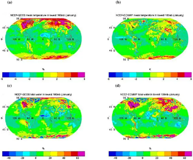
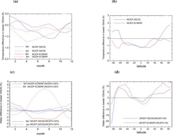
Fig. 1. (a) Map of the differences between the mean temperature in the lowest 100mbar of the atmosphere as given by GEOS from that given

by NCEP/NCAR. (b) Same as in (a), but for ECMWF instead of GEOS. (c) Same as 1a, but for water vapour in the lowest 100 mb of the atmosphere. (d) Same as (c), but for ECMWF instead of GEOS.

climatology dataset gives the detailed information on cloud properties provided by ISCCP and required by the model.

Another cloud parameter which is necessary for the es-timation of the downwelling flux at the surface and which is not provided by satellite data is the cloud-base temper-ature. This parameter is estimated (as in Hatzianastassiou et al., 1999) from the ISCCP-D2 cloud-top pressure and the cloud physical thickness values given by Peng et al. (1982).

The vertical temperature and humidity profiles (including surface pressure) were taken from three different reanalyses projects: (i) NCEP/NCAR (National Center for Environmen-tal Prediction/National Center for Atmospheric Research Re-analysis project, see Kistler et al., 2001); (ii) ECMWF (Euro-pean Centre for Medium-Range Weather Forecasts Reanaly-sis); and (iii) GEOS-1 Reanalysis (Goddard Earth Observing System, see Schubert et al., 1995). All data were monthly averaged and remapped to match the 2.5-degree resolution of the ISCCP-D2 dataset. Table 1 summarizes the various sources of input data used in the present study and their

ba-sic characteristics. The model runs with the three different datasets are referred to as case-i, case-ii and case-iii, respec-tively.

Finally, the total amounts and vertical distribution of ozone, carbon dioxide, methane, and nitrous oxide in the atmosphere are taken from Hatzianastassiou and Var-davas (2001) and references therein.

Aerosols are not currently included in the calculations of the DLF. Although inclusion of the aerosol effect could be significant in specific regions (e.g. in the Sahara, or over biomass burning regions), on the whole it is not expected to affect our analysis substantially (see for example Morcrette, 2002; Zhou and Cess, 2000).

2.3 Inter-comparison of temperature and specific humidity datasets

Air temperature: especially of the lower atmospheric layer, plays an important role in determining the DLF reaching the surface. In Fig. 1a we show, as an example, the global

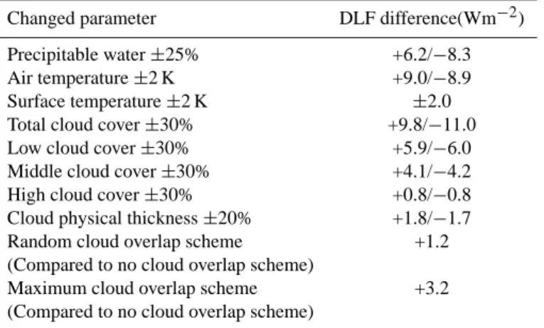
Table 2. Summary of results of the sensitivity analysis performed

Changed parameter DLF difference(Wm−2)

Precipitable water ±25% +6.2/−8.3

Air temperature ±2 K +9.0/−8.9

Surface temperature ±2 K ±2.0

Total cloud cover ±30% +9.8/−11.0

Low cloud cover ±30% +5.9/−6.0

Middle cloud cover ±30% +4.1/−4.2

High cloud cover ±30% +0.8/−0.8

Cloud physical thickness ±20% +1.8/−1.7 Random cloud overlap scheme +1.2 (Compared to no cloud overlap scheme)

Maximum cloud overlap scheme +3.2 (Compared to no cloud overlap scheme)

distribution of the difference between the mean temperature of the lowest 100 mbar of the atmosphere given by GEOS and that given by NCEP/NCAR, for the month of January

1_{. The largest differences reaching values of 6 K (with}

NCEP/NCAR giving the higher values) occur over land, par-ticularly in extended regions of the Northern Hemisphere in winter (North America, Siberia, Antarctica), while over oceans the differences are smaller, of the order of 1 K. The discrepancies between NCEP/NCAR and ECMWF are gen-erally less pronounced (Fig. 1b). Again, best agreement is encountered over oceans, as also found by Anyamba and Susskind (1998), while differences of up to 4 K can be found over land, especially in high altitude- regions (Andes, Green-land, Tibetan plateau, Antarctica).

Figure 2a shows the seasonal dependence of the long-term averaged temperature (of the lowest 100 mbar) bias between the different databases, plotted separately for the Northern and Southern Hemispheres. Globally, both GEOS and ECMWF give higher temperatures than NCEP/NCAR in the lowest 100 mbar of the atmosphere. Significant sea-sonality is displayed by the NCEP/NCAR-GEOS bias in the Northern Hemisphere (solid blue curve in Fig. 2a), and by the NCEP/NCAR-ECMWF bias in the Southern Hemisphere (dashed red curve in Fig. 2a). In the former case, the lowest bias is observed in winter months and the highest in August and September, while in the latter the highest bias is in April and the lowest bias in (southern) summer.

Figure 2b shows the latitudinal dependence of the an-nual long-term zonally averaged temperature (of the lowest 100 mbar) bias between the different databases. On average, GEOS and ECMWF show no systematic difference between

−40◦and 40◦, while they both give higher temperatures, by 1 K, than NCEP/NCAR, in the same zone. On the contrary, in high latitudes of the Northern Hemisphere (50◦N–80◦N) the NCEP/NCAR temperature has a mean annual value of

∼1 K greater than GEOS.

1_{Longterm average for the years common in the two datasets}

Specific Humidity: The differences between water vapour content in the lowest 100 mb of the atmosphere given by the three databases are typically about 25% over much of the globe, although there are extended regions in the Northern Hemisphere mostly above 40◦ _{(North America and Asia),} where there are much larger differences, that exceed 60%.

As an example, we show the global distribution of the wa-ter vapour difference between NCEP/NCAR and GEOS, and NCEP/NCAR and ECMWF, in Figs. 1c and d respectively, for the month of January. The large discrepancies in the Northern Hemisphere between NCEP/NCAR and ECMWF are obvious in Fig. 1d, however they are much reduced (to 15%) during summer.

Figure 2c shows the seasonal dependence of the long-term averaged water vapour content (in the lowest 100 mbar) bias between the different databases, plotted separately for the Northern and Southern Hemispheres.

Generally, there is a strong seasonality in the water vapour difference between NCEP/NCAR and ECMWF (red curves). In the Northern Hemisphere, the water vapour given by NCEP/NCAR is more than that of ECMWF for the winter months, while the reverse occurs in sum-mer. In the Southern Hemisphere, the seasonal depen-dence is even stronger (dashed red curve), with large positive NCEP/NCAR-ECMWF bias in (southern) winter and nega-tive bias in summer. There is no such pronounced seasonality in the water vapour difference between the NCEP/NCAR and GEOS databases.

Figure 2d shows the latitudinal dependence of the an-nual long-term zonally averaged water vapour (in the lowest 100 mbar) bias between the different databases. On average all three databases show better agreement (within 2–5%), in the tropics, with ECMWF giving the highest water vapour values, followed by GEOS and then by NCEP/NCAR. At mid-latitudes, the discrepancies are larger, reaching 10–12%, with ECMWF giving the lowest values of water vapour, fol-lowed by GEOS and then by NCEP/NCAR.

(a) (b)

(c) (d)

Fig. 2. (a) Seasonal dependence of the long-term averaged temperature (in the lowest 100 mb of the atmosphere) difference between

NCEP/NCAR and GEOS (blue curve), and between NCEP/NCAR and ECMWF (red curve), for the Northern Hemisphere (solid line) and for the Southern Hemisphere (dashed line). (b) Latitudinal dependence of the annual long-term zonally averaged temperature (of the lowest 100 mbar) bias between NCEP/NCAR and GEOS (blue curve), and between NCEP/NCAR and ECMWF (red curve). (c) Same as (a), but for water vapour in the lowest 100 mb of the atmosphere. (d) Same as (b), but for water vapour in the lowest 100 mb of the atmosphere.

3 Model Sensitivity Analysis

A series of sensitivity tests were performed to investigate how much uncertainty is introduced to the model down-welling longwave fluxes by uncertainties in the input param-eters. Each test calculation covers the entire globe for one month. The results are summarised in Table 2.

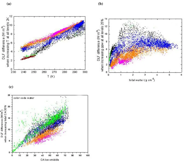
Atmospheric temperature profile: We have run a sensitiv-ity test examining the effect on the DLF of an increase (or decrease) in the air temperature by 2 K2(the entire profile is moved to higher/lower temperature). It was found that such an increase causes an increase of the global average DLF by 9 Wm−2(or decrease of 8.9 Wm−2), as shown in Ta-ble 2. This is similar in magnitude to the results by Zhang et al. (1995) using the GISS radiation transfer model. On grid-box level (Fig. 3a), the increase of the DLF, caused by a 2 K atmospheric temperature increase, ranges from 2 Wm−2to 11 Wm−2depending on the climatic conditions, i.e. on tem-perature, cloud cover and water vapour content. For the fixed

2_{This is the typical value of the difference between temperatures}

given by the three reanalyses datasets

2 K increase, the weakest effect (about 2 Wm−2)is observed in very cold climates with very low cloud cover (practically clear sky), while the largest effect (about 10 Wm−2)occurs in hot and cloudy (mainly tropical) regions. In each tempera-ture regime there is a range of about 3 Wm−2in the observed DLF difference, caused mainly by cloud amount differences.

3

Specific Humidity: We have run a sensitivity test in which we have increased (or decreased) by 25%4the specific hu-midity in each atmospheric layer for each grid-box. The re-sulting global increase in the DLF is 6.2 Wm−2(or decrease by 8.3 Wm−2) on average, with differences ranging from 1 to 14 Wm−2. Grid-boxes with originally low water vapour con-tent are obviously the least affected. For example, for grid-boxes with (total) precipitable water less than 0.5 g cm−2, the average increase of the DLF in the above test was 3 Wm−2_. 3_{The apparent bifurcation in DLF difference observed for very}

low temperatures in this figure is caused by an actual absence of grid-boxes with low/middle cloud cover between 10 and 30%.

4_{This is the typical value of the difference between water vapour}

(a) (b)

(c)

Fig. 3. (a) The increase in DLF when the temperature of the atmosphere is increased by 2 K at all levels, as a function of mean temperature

in the lowest 100 mbars of the atmosphere. The colour coding refers to low plus middle cloud cover: brown is for CA<5%, green is for CA between 5% and 10%, black is for CA between 10% and 30%, blue is for CA between 30% and 50%, orange is for CA between 50% and 70% and magenta is for CA>70%. (b) The increase in DLF when precipitable water of the atmosphere is increased by 25% at all levels, as a function of total precipitable water (prior to the increase). The colour coding refers to low plus middle cloud cover: green is for CA<10%, black is for CA between 10% and 30%, blue is for CA between 30% and 50%, orange is for CA between 50% and 70% and magenta is for CA>70%. (c) The increase in DLF when cloud cover increases by 30% of its given value, as a function of original cloud (low and middle-level) cover. The colour coding refers to: green is for precipitable water less than 0.5 g cm−2, black is for precipitable water between 0.5 and 1 g cm−2, blue is for precipitable water between 1 and 2.5 g cm−2, orange is for precipitable water between 2.5 and 4 g cm−2and magenta is for precipitable water larger than 4 g cm−2.

The response of the DLF to water vapour changes clearly de-pends also on temperature -with the colder regions the least affected- and on low and middle cloud cover, since, when cloud is present, water vapour thermal emission that reaches the surface, comes from a much smaller column. For exam-ple, for precipitable water between 1 and 2 g cm−2, the in-crease in DLF due to a 25% inin-crease in precipitable water, is about 3 Wm−2_{, on average, for grid-boxes with cloud cover}

larger than 70%, while it rises to 12 Wm−2_{for grid-boxes}

with cloud cover less than 10%. This coupling between low and middle cloud cover and DLF sensitivity to water vapour

changes is shown in Fig. 3b. Fasullo and Sun (2001)5also noted the role of the presence of low clouds in determining the sensitivity of the DLF and found that the largest sen-sitivity of the DLF on water vapour is encountered in the dry zones of the subtropics and eastern Pacific Ocean. An-other effect that can be seen in Fig. 3b is that in regions with large water vapour content, i.e. larger than approximately 3 g cm−2_{(mostly in the tropics) the DLF sensitivity becomes}

saturated, as the infrared emissivity of the water vapour layer

5_{Based on the CCM3 radiation code, on ISCCP-C2 cloud}

increases towards unity. So, in these regions, the DLF only rises by 5–8 Wm−2_{, irrespective of variations in cloud cover}

and water vapour, and in spite of the high temperatures. Cloud cover: Satellite cloud-cover uncertainties can be quite large. Threshold temperature and reflectivity are used to identify clouds from satellite measurements. As a re-sult, the fractional cloud cover can differ greatly among var-ious data sets depending upon the threshold values used. As shown by Stowe et al. (2002), for example, the (abso-lute) difference in total cloud cover between ISCCP-D and NOAA/PATHFINDER (PATMOS) is quite large, reaching 15% in the tropics (with ISCCP giving on average 65% to-tal cloud cover and PATMOS giving about 50%) and almost 35% at the poles (with ISCCP-D giving on average 60% to-tal cloud cover and PATMOS6giving about 95%). We have therefore run a test to examine the sensitivity of the DLF to possible errors in the cloud data. We have changed the to-tal cloud amount by ±30% of its value for each grid-box and found that the global mean value of the DLF at the sur-face changed by ±10 Wm−2. If just the low cloud amount is changed by ±30%, the effect on the global average DLF is ±6 Wm−2 _{while if the middle cloud amount is changed}

by ±30%, the effect on the DLF is less but comparable to the low cloud case (±4 Wm−2). For the high cloud cover the effect is, expectedly, much less significant (±0.8 Wm−2). Close examination of the effect on a grid-box basis shows that the difference in the DLF ranges from 0 to 25 Wm−2, depending on original (low and middle) cloud cover, water vapour content and temperature. For the same amount of cloud cover, the less the amount of water vapour is in the lower atmosphere, the higher the increase in the DLF caused by the increase in cloud cover (see Fig. 3c). Temperature plays a secondary role (and therefore its effect is not shown in Fig. 3c). For example, the warmest regions, in which the mean temperature of the lower part of the atmosphere is larger than 290 K, show the lowest sensitivity to the cloud cover increase. This is due to the fact that in these same re-gions generally the water vapour content of the atmosphere is very high, which in conjunction with high atmospheric tem-peratures leads to a significant contribution to the DLF under clear-sky conditions. On the other hand, cold regions (mean T<270 K) with low water vapour content are the most af-fected by an increase in cloud cover. This is an important re-sult, given that the most severe discrepancies in cloud cover between different datasets, mentioned above, occur in cold climates.

For example, the mean difference of about 60% in cloud cover between PATMOS and ISCCP-D in Antarctica, can produce differences in the DLF of about 40 Wm−2. On the other hand, the 30% difference in cloud cover between the two datasets in the tropics would lead to discrepancies in the DLF, only of about 5–10 Wm−2.

6_{The PATMOS cloud data do not include information on}

indi-vidual cloud types or properties.

The three plots given in Fig. 3, and discussed in the pre-vious paragraphs, can be used effectively for assessing the sensitivity of the DLF to temperature, precipitable water and cloud amount, for specific geographical regions (with spe-cific climatic conditions).

Cloud-physical thickness: This quantity, taken from Peng et al. (1982), determines along with the cloud-top pres-sure provided by the satellite meapres-surements, the cloud-base height, which in turn specifies the cloud-base temperature. We ran a sensitivity test in which we increased (or decreased) the cloud physical thickness by 20%, which caused a cor-responding lowering (or rising) of the cloud base. As a consequence, the global average DLF increased (decreased) by 2 Wm−2. Similar values were also found by Zhang et al. (1995). On a grid-box level, the change in DLF ranges between −1 and 4.5 Wm−2_{, with most of the grid-boxes}

hav-ing values between 1 and 3 Wm−2_{. Further, there is a}

depen-dence of the sensitivity of the DLF (caused by the change of the cloud base) on cloud cover, as expected, but it is not very strong. Some negative changes occur in a few grid-boxes in polar regions with temperature inversions, where the original cloud base happened to coincide with the local maximum in the temperature profile.

Cloud overlap scheme: One known limitation of the ISCCP-D2 dataset is the assumption that the clouds are clas-sified into non-overlapping layers. From the satellite point of view, if there are low clouds under the optically thick middle clouds, they will not be observed. This fact leads to a systematic underestimation in low-level cloud amount, and consequently in DLF at the surface. In order to ex-amine the possible effect that this assumption has on the DLF, we implement two cloud-overlap schemes, based on random and maximum overlap, corresponding to the ran-dom and maximum overlap with no-constraints, described in Chen et al. (2000). The random-overlap scheme assigns lower cloud amounts under higher clouds, based on cloud cover in areas where the satellite’s view to the lower cloud is not obscured. The maximum-overlap scheme assumes that a lower cloud always exists under the higher cloud. Over-all, the random overlap assumption seems to be the prefer-able procedure (Zhou and Cess, 2000). Application of the random-overlap scheme leads to an increase of the DLF by about 1.2 Wm−2on average, globally, while the maximum-overlap scheme leads, expectedly, to a larger increase of 3.2 Wm−2, as shown in Table 2. The maximum effect on the DLF reaches 8 Wm−2_{, for the random overlap scheme and}

is observed in areas where originally both low and middle cloud cover is significantly high. This value is comparable to the effect reported by Chen et al. (2000), but it is signifi-cantly lower than the value of 20 Wm−2reported by Zhou and Cess (2000). For the maximum overlap scheme, the maxi-mum effect on the DLF reaches 14 Wm−2in specific regions, although the median value is only 2.9 Wm−2over most of the globe.

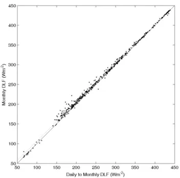
Fig. 4. Comparion between the monthly DLFs derived from monthly climatologies, against the monthly DLFs derived by av-eraging the daily DLFs. The dashed line is the least squares best fit line, while the solid line shows a slope equal to 1.

Temporal resolution: As mentioned in Sect. 2, in this study we use mean monthly climatological data as input to our model. The climate processes, however, often display non-linear behavior, so we examined the effect that monthly av-eraging has on the estimation of fluxes by the model. Specif-ically, we ran the model with daily data, producing daily fluxes and averaging these to derive monthly fluxes. These fluxes were compared with those derived by the model when mean monthly climatological data were used to produce the monthly fluxes. The sensitivity test was performed using daily data for physical quantities that significantly affect the DLF, i.e. the cloud amounts, and the vertical temperature and humidity profiles of the atmosphere. All these parame-ters are provided at BSRN stations with temporal resolution of a few minutes. We produced daily cloud amounts and vertical atmospheric profiles from these datasets and ran the daily model for 12 stations, covering a range of climates from tropical to polar, which had the necessary data. In Fig. 4, we compare the monthly DLFs derived from monthly clima-tologies, against the monthly DLFs derived by averaging the daily DLFs. The least squares best fit line is shown with a dashed line and has a slope of 0.981±0.004, at the 95% con-fidence level. The solid line shows a slope equal to 1, for comparison. The average difference between the two sets of monthly fluxes is 3.5 Wm−2, while the standard deviation of the differences is 4.8 Wm−2.

4 Model results

The model was run for all three different input meteorolog-ical reanalysis data sets: NCEP/NCAR (cases-i), ECMWF (case-ii) and GEOS (case-iii). Cloud data were taken from ISCCP-D2 for all three cases.

4.1 Geographical Distribution

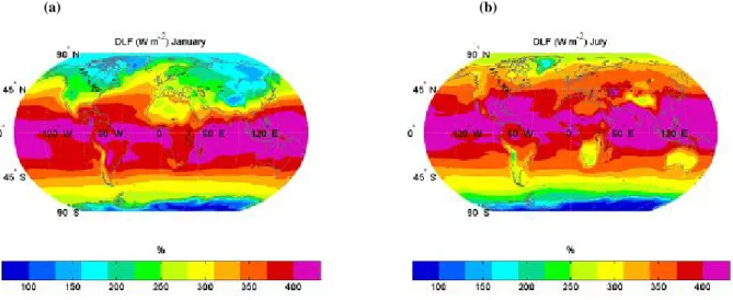
Case-i: The resulting geographical distribution of the 10-year average of the DLF, for case-i, is shown in Figs. 5a and b for two months (January and July). As expected, in January, the maxima of DLF occur over a broad swath along the equator, mainly over tropical and subtropical oceans along the inter-tropical convection zone. In these regions cloud amounts, water vapor and air temperatures are high, while cloud bases are low. The maxima are shifted slightly northwards in July. Minima occur, as expected, in the polar regions, with Antarc-tica and Greenland having the lowest values, and over an ex-tended area in the Northern Hemisphere in winter. A lower seasonal variability is seen in the Southern Hemisphere com-pared with that in the Northern Hemisphere. Note the re-gional minima of the DLF in winter over dry desert areas (Sahara, Atacama, Kalahari, Central Australia), character-ized by clesky conditions, as well as over high-altitude ar-eas (Tibetan Plateau, Rocky Mountains, Andes, Greenland, Antarctica), with low cloud cover, low air temperatures, and low moisture content.

Case-ii : The global distribution of the DLF generally has the same characteristics as for case-i. Figure 6a shows the global distribution of the difference in DLF between case-i and case-ii, for the month of January, as an example. Gen-erally, the differences are about 10 Wm−2or less, over most of the globe. The scatter around the best-fit line represent-ing DLFcase−i vs DLFcase−ii (for all individual grid-boxes)

is 5.4 Wm−2. However, there are regions where the differ-ence between them can reach values as large as 30 Wm−2, with DLFcase−ibeing significantly higher over high attitude

regions such as the Tibetan plateau, the Andes, the Rocky Mountains, as well as in Eastern Africa. Comparison with Fig. 1d, shows that these discrepancies are mainly connected to differences in water vapour. However, similarly large dif-ferences in water vapour (Fig. 1d) exist also over extended regions of North America and Siberia, although the corsponding DLFs are in relatively good agreement. This re-flects the relatively low sensitivity of the DLF to the water vapour content in the lowest 100 mbar of the atmosphere, in regions with large (over 50%) low cloud amount (see Sect. 3).

Case-iii: As for case-ii, the global distribution of the DLF is similar to case-i for most of the globe, however there are large differences over specific regions. Figure 6b shows the difference between cases iii and i, again for January. The most pronounced differences occur in India, Sahel, and the Andes, where the (absolute) differences exceed 20 Wm−2,

(a) (b)

Fig. 5. (a) Geographical distribution of model downwelling longwave flux, DLF, at the surface for January, averaged over 1984–1993, for

case-i; (b) Same as Fig. 1 but for July.

linked to large water vapour differences (Fig. 1c). There are also relatively large differences over high latitude land in the Northern Hemisphere, due to temperature differences (Fig. 1a). The scatter around the best-fit line represent-ing DLFcase−ivs DLFcase−iii (for all individual grid-boxes)

is 5.3 Wm−2_{. The differences between cases ii and iii are}

mapped over the globe in Fig. 6c. The most significant dif-ferences (of the order of 30 Wm−2)occur in the Northern Hemisphere in the Sahel, the Tibetan plateau as well as in the Andes where case-iii fluxes are higher than case-ii fluxes. On the other hand, in the Southern Hemisphere the differ-ences are of the opposite sign, and are more pronounced over the oceans at mid-latitudes. The scatter around the best-fit line representing DLFcase−iivs DLFcase−iii(for all individual

grid-boxes) is 6.8 Wm−2.

In Figs. 6a, b and c the differences are relatively large in specific regions, although globally the agreement is good, with the rms of the difference between the DLFs of different cases ranging from 5 to 6.8 Wm−2. Some of these regions are areas with rough topography, so the differences between the DLFs may not be entirely due to differences in the databases, but may be partly caused by the remapping of the original databases onto a 2.5×2.5 degree grid. We are currently pro-cessing 1×1 degree climatologies from NASA-Langley and will be able to investigate this issue further in a future work.

4.2 Latitudinal and Seasonal inter-comparison

Figure 7a shows the latitudinal dependence of the annual long-term zonally averaged difference between the DLFs de-rived by the different model runs. Generally, DLFcase−iiand

DLFcase−iiishow relatively small differences in all latitudes

(except for the polar regions). However, larger discrepancies occur between DLFcase−iand the other two cases, particularly

in the tropics 20 S–20 N, where the difference in the zonal

average DLFs reach 6–8 Wm−2. This difference is caused primarily by the fact that both GEOS and ECMWF have tem-peratures (in the lowest 100 mb) higher by 1 K (Fig. 2b) on average than NCEP/NCAR in the tropical zone and secon-darily by the ∼4% difference in water vapour (Fig. 2d). In mid latidudes (30◦_–60◦_{)the differences between the DLFs} are less than 2 Wm−2_.

Figure 7b shows the seasonal dependence of the long-term mean hemispherical difference between the DLFs derived by the different model runs, plotted separately for the northern (solid lines) and southern (dashed lines) hemisphere.

The DLFcase−i–DLFcase−ii difference shows strong

sea-sonal dependence in both hemispheres, following the strong seasonality of the water vapour difference between the cor-responding input databases (Fig. 2c). Less pronounced, but significant, is the seasonal dependence of the DLFcase−i–

DLFcase−iiidifference, which is caused mainly by the

season-ality in the difference between the NCEP/NCAR and GEOS temperatures (in the lowest 100 mb), as is seen in Fig. 2a.

4.3 DLF Time-series

Figure 8a shows the time-series of the global average value of the monthly DLF for the ten year period 1984–1993, for all three cases. The large regional discrepancies are smoothed out when considering global means. Thus the differences in the global average monthly values are only of the order of 1–2%. It is also obvious from Fig. 8a that all three datasets follow overall the same seasonal variability, with the maxima corresponding to Northern Hemisphere Summer.

In Fig. 8b, we present the time-series of the difference of the DLF time-series between case-ii and case-i, between case-iii and case-i and between case-ii and case- iii. The lat-ter pair shows the best agreement. It should also be noted that although the difference between case-ii and case-iii DLF

(a) (b)

(c)

Fig. 6. (a) Global map of the difference between the downwelling longwave fluxes calculated by case-ii [vertical profile of precipitable water

and temperature from ECMWF reanalysis] and case-i [vertical profile of precipitable water and temperature from NCEP/NCAR reanalysis], for January. (b) Global map of the difference between the downwelling longwave fluxes calculated by case-iii [vertical profile of precipitable water and temperature from GEOS reanalysis] and case-i, for January. (c) Global map of the difference between the downwelling longwave fluxes calculated by case-iii and case-ii, for January.

is relatively small, it is of opposite signs for the periods be-fore and after 1989, resulting in a small decadal trend. Both case-ii and case-iii give systematically higher DLF globally by about 2 Wm−2than case-i.

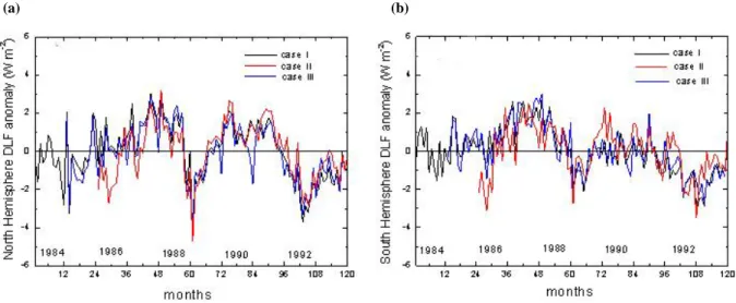
Figure 9 shows the time series of the anomaly of the mean monthly DLF at the surface of the earth for the period 1984– 1993 for the northern (Fig. 9a) and the southern (Fig. 9b) hemispheres. All three cases show similar interannual vari-ations of the DLF, in both hemispheres, with a broad maxi-mum corresponding to the 86/87 El Ni˜no episode, followed by a well-defined minimum related to the 89/90 La Ni˜na event. There is no strong signature of the 91/92 El Ni˜no event, although there is an increase in the flux compared to 89/90. It is possible that the Pinatubo eruption in June 1991 may have caused a depression in the DLF, more or less co-incident with the 91/92 El Ni˜no event: The aerosols from

this eruption caused a decrease in solar heating, which led to a global cooling of the lower troposphere, and an associ-ated reduction in global water vapour concentrations (Soden et al., 2002).

Finally, all three cases show a well defined minimum in the second part of 1992, mainly in the Northern Hemisphere. The case-ii anomaly time-series shows a broad significant minimum in 1986 in both hemispheres, which however is not shown by the other two time-series. On the other hand, the case-iii anomaly time-series shows two narrow minima at the end of 1989 and end of 1990, again not seen in the other time-series. Flux variations not seen in all three cases (i.e. based on input data from the three different reanalyses), and in both hemispheres should be given lower confidence (see e.g. Kistler et al., 2001).

(a) (b)

Fig. 7. (a) Latitudinal dependence of DLFcase−i–DLFcase−ii(red line), and DLFcase−i–DLFcase−iii(blue line). (b) Seasonal dependence

of DLFcase−i–DLFcase−ii (red line), and DLFcase−i–DLFcase−iii(blue line) for the Northern Hemisphere (solid lines) and the Southern

Hemisphere (dashed lines).

(a) (b)

Fig. 8. (a) Time series of the global average of the DLF for a period of 120 months (from January 1984 to December 1993), as calculated

by the model for the three different cases of input parameters: case-i, black line; case-ii, red line and case-iii, blue line. (b) Time series of the DLF differences between the three cases: case-ii minus case-i (red line), case-iii minus case-i (blue line) and case-ii minus case-iii (black line).

5 Comparison with long-term averages of other models

The global long-term average of the DLF reaching the sur-face of the Earth is 342.2 Wm−2for case-i, 344.3 Wm−2for case-ii and 343.9 Wm−2for case-iii, respectively.

The hemispherical and global long-term averages of the DLF for all three cases are given in Table 3, along with re-sults of other recent calculations, based either on determistic models, or on general circulation models. We also in-cluded in the Table the global average of the DLF at the sur-face as estimated from GEBA station measurements. The global long-term averages and the hemispherical values cal-culated here are in good agreement with recent results from

other deterministic radiation transfer models using satellite data. Our global long-term average is somewhat lower (by about 4 Wm−2for case-iii) than the values derived by Gupta et al. (1999) and by Rossow and Zhang (1995). As far as comparison with GCM results is concerned, we mention here the excellent agreement with ECHAM4 (Wild et al., 2001) that has been shown to provide better agreement with obser-vations than many other GCMs, examined in detail by Wild et al. (1998) and Garratt et al. (1998). Very good agree-ment is also found with the CSU/GCM of Randall (1997), as quoted by Gupta et al. (1999), while CCM3 gives about 7 Wm−2less DLF than found here. An improvement to the CCM3 radiation code has been employed recently (Iacono

(a) (b)

Fig. 9. Time-series of hemispherical DLF anomaly over the ten-year period 1984–1993. The black line corresponds to case-i, the red line to

case-ii and the blue line to case-iii. (a) Northern Hemisphere, (b) Southern Hemisphere.

Table 3. Hemispherical and global long-term averages of the DLF at the surface as found in the present study, and in other recent studies.

Reference DLF (Wm−2) NH DLF (Wm−2) SH DLF (Wm−2) Global comment Deterministic models

Present study 343.3 341.1 342.2 1984–1993 FORTH-model Case-i

” 345.2 343.4 344.3 1985–1993 FORTH-model Case-ii

” 345.3 342.6 343.9 1986–1993 FORTH-model Case-iii

Rossow and Zhang (1995) 348.0 modified GISS code with ISCCP-C1 data

Gupta et al. (1999) 351.0 344.6 347.8 Gupta model with ISCCP-C1 data

Hatzianastassiou and Vardavas (2001) 341.0 FORTH zonal model with ISCCP-C2 data

Hatzianastassiou et al. (2001b) 331.5 Zonal FORTH model with ISCCP-D2 data

General circulation models

Wild et al. (2001) 344.0 ECHAM4 GCM

Wild et al. (2001) 337.0 HadAM2 GCM

Wild et al. (2001) 333.0 HadAM3 GCM

Garratt et al. (1998) 339.0 CSIRO-2 GCM

Randall (1997), as given 343.7 337.2 340.8 CSU GCM

in Gupta et al. (1999)

Zhang (1997),as given 335.1 332.7 333.9 CCM3 GCM

in Gupta et al. (1999)

ECMWF 339.3 339.9 339.6 ERA-15 GCM

Surface stations

Ohmura (2003) 345.0 GEBA & BSRN

private communication

et al., 2000) which has led to an increase of the DLF fluxes at the surface by 8–15 Wm−2at high latitudes and other dry regions, which will in turn reduce the bias between our re-sults and the CCM3 rere-sults. A host of other GCMs (e.g. HadAM2b, HadAM3, ERA, CSIRO) also shown in Table 3 give values that are generally lower than our value by about 8–14 Wm−2.

6 Validation against BSRN station data

Validation of model results for the downward flux reaching the surface of the Earth is only possible through comparison with ground-based measurements at specific sites. To this aim we have used ground-based observations taken from the Baseline Surface Radiation Network (BSRN, Ohmura et al., 1998).

Table 4. List of BSRN stations used to validate the model derived downwelling longwave fluxes.

Station Name Latitude (◦) Longitude (◦) Elevation (m) Period

Ny- ˚Alesund, Norway 78.92 11.95 11 1992–1996

Barrow, Alaska 71.32 −156.61 8 1992–2001

Payerne, Switzerland 46.82 6.94 491 1992–1996

Boulder, Colorado 40.05 −105.01 1577 1992–2001

Bermuda 32.30 −64.77 8 1992–2001

Kwajalein, Marshall Isl. 8.72 167.73 10 1992–2000

Ilorin, Nigeria 8.53 4.57 350 1992–1995

Neumayer, Antarctica −70.65 −8.25 42 1992–1996

Table 5. Validation of model vs. BSRN measured DLF for the three different runs. Bias is the mean difference between model and station

fluxes, RMS is the root mean square difference, Slope is the slope of the least squares line. The value intervals correspond to 95% confidence. All values except the slope are in Wm−2.

Model Run Bias (Wm−2) RMS(Wm−2) Slope

ISCCP-D2 cloud climatologies and −8.3 19.4 1.12±0.03 NCEP/NCAR temperature and

humidity profiles [case-i]

ISCCP-D2 cloud climatologies −7.9 22.6 1.14±0.04 and ECMWF temperature and

humidity profiles [case-ii]

ISCCP-D2 cloud climatologies and −6.6 21.3 1.19±0.03 GEOS temperature and

humidity profiles [case-iii]

Model DLFs (for all three cases of input reanalysis data) were compared against BSRN fluxes. Data from 8 BSRN sta-tions7(Table 4) were used for this purpose. In Fig. 10, we show the corresponding scatter plot, comparing model fluxes (for case-ii model fluxes as an example) against station mea-surements. Similar scatter plots were also constructed for cases i and iii. Table 5 lists the results of the comparison between model and BSRN station DLFs for all three cases. There is a negative bias of the model fluxes when compared against BSRN fluxes, ranging from −7 to −9 Wm−2. It must be emphasized here that although the number of BSRN stations used for the comparison is small, the geographi-cal distribution of these stations represents a wide variety of climates. The slope of the line best fitted to the data is marginally larger than 1, indicating that low fluxes are under-estimated and high fluxes are somewhat overunder-estimated. This underestimation of DLF in cold and dry climates seems to be caused by a clear-sky bias of our simple radiation scheme, found also with other simple radiation codes used in GCMs and reanalyses as reported in Wild et al. (2001). The scatter around the best fit line in Fig. 10, ranges from 19 Wm−2to 23 Wm−2. The smallest bias is displayed by case-iii, while the smallest scatter is displayed by case-i, which also

dis-7_{These are the only BSRN stations that have longwave flux}

mea-surements within the period 1984–1993.

plays the smallest deviation from a slope of 1. It must be noted that the model fluxes have been slightly adjusted, prior to the comparison against station fluxes, to account for any elevation difference between the station site and the much larger 2.5◦×2.5◦grid box. We adopted a height gradient of 2.8 Wm−2(100 m)−1(Wild et al., 1995) to allow for this ef-fect.

The observed biases could be due to two factors, a) model deficiencies and b) input data errors. By input data errors we mean either input data problems, or that the grid box and sta-tion have different climatic condista-tions. In order to determine which one of factors a) and b) is predominant, we ran the model with locally observed cloud fractions and radiosonde profiles for the temperature and humidity and compared the resulting DLF against the BSRN measured DLF. This ex-periment is run for BSRN stations for which cloud fractions and radiosonde measurements were recorded routinely. The model bias was significantly reduced to −2.4 Wm−2_{, with a}

scatter of only 11.6 Wm−2_{, showing that the model is able to}

reproduce the observed DLF at a specific station very well, when run with the local data.

Fig. 10. Comparison between BSRN DLF and model case-i DLF.

The dashed line is the line best fitted to the data.

Fig. 11. Dependence of model DLFcase−i over/underestimation

with respect to BSRN station measurements on the difference be-tween ISCCP-D2 low cloud amount and BSRN synoptic low cloud amount measurements.

Further analysis showed that the mismatch between model and BSRN fluxes was related in most cases to low cloud cover and less frequently to temperature and specific hu-midity differences. Although the ISCCP low-level cloud amounts generally agree with the ones observed at the BSRN locations, sometimes they are substantially lower,

particu-larly at mid and high latitudes in winter, i.e. at the low end of the DLF scatter plot. There is a clear correlation between the model underestimation of the DLF and the underestimation of low-level cloud cover by ISCCP D2. We see that as the differences between the ISCCP D2 and the BSRN low-level cloud amount decrease, so do the differences between model and BSRN DLF (Fig. 11).

7 Summary

Downwelling longwave fluxes, DLFs, have been derived for each month over a ten year period (1984–1993), on a global scale with a resolution of 2.5×2.5 degrees. The fluxes are available on the World Wide Web at http://esrb.iesl.forth.gr/ LW-Fluxes.

The fluxes were computed using a deterministic model for atmospheric radiation transfer, along with satellite and re-analysis data for the key atmospheric input parameters, i.e. cloud properties, and specific humidity and temperature pro-files.

The cloud climatologies were taken from the latest re-leased and improved International Satellite Climatology Project D2 series. Specific humidity and temperature vertical profiles were taken from three different reanalysis datasets; NCEP/NCAR, GEOS, and ECMWF (acronyms explained in main text).

A series of sensitivity tests were performed to investigate how much uncertainty in the DLF can be caused by uncer-tainties in the input data. This sensitivity was investigated regionally, as well as globally. The maximum sensitivity of the DLF to a temperature increase (or decrease) occurs in the tropics, where there is high water vapour content and signif-icant cloud cover. In these regions, the DLF can increase by up to 11 Wm−2_{for a 2 K temperature increase. The}

sen-sitivity of the DLF to water vapour increase (or decrease) depends crucially on the amount of low and middle cloud cover. The maximum sensitivity of the DLF to changes in the water vapour content of the atmosphere occurs over areas with little cloud cover and precipitable water values between 1–2 g cm−2(deserts). In these regions, the DLF can increase by up to 25 Wm−2for a 25% increase in precipitable water. The sensitivity to the same percentage of precipitable water increase is much smaller, about 5–8 Wm−2, in the tropics, despite the high temperatures and high water vapour content in these regions. The sensitivity of the DLF to differences in cloud cover values depends primarily on water vapour and secondarily on temperature. Cold regions with low water vapour content are the most affected by an increase in cloud cover, while the opposite is true for hot and humid (tropical) regions. Finally, uncertainties in cloud physical thickness of about 20% do not affect significantly the DLF.

DLFs were computed separately for all three reanaly-sis temperature and specific humidity datasets. The tem-perature and specific humidity data (particularly for the

lower troposphere) as well as the resulting fluxes were inter-compared. Significant regional differences between the three reanalyses were noted both in temperature and in specific hu-midity (in the lower troposphere), over land, particularly over high altitude and dry regions. The combined effect of these differences on the regional DLFs can reach 30 Wm−2in spe-cific regions, however, globally the agreement is good, with the rms of the difference between the DLFs derived from the three reanalysis datasets ranging from 5 to 6.8 Wm−2. Gen-erally, the DLFs derived using GEOS and ECMWF reanal-ysis data are in better agreement between themselves, than with the DLFs derived on the basis of NCEP/NCAR reanal-ysis.

The results are presented as geographical distributions and as time series of hemispheric and global averages. The DLF time series based on the different reanalysis datasets show similar seasonal and inter-annual variations. Anoma-lies caused by the 86/87 El Ni˜no and 89/90 La Ni˜na events, are clearly seen in all cases. Therefore, although for regional studies, there are significant differences, for longterm climate studies all model runs (using the different reanalyses temper-ature and humidity data) give similar results, at least over the 10 year period examined in the present study.

The global ten-year average of the DLF was found to be 342.2 Wm−2 when using NCEP temperature and humidity data, 344.3 Wm−2with ECMWF data, and 343.9 Wm−2with GEOS data. These agree very well with the ECHAM 4 value, but it is generally larger than most other GCM results. It is however lower than other deterministic model results, such as the results of Gupta et al. (1999).

Our model downwelling fluxes are validated against avail-able data from ground-based stations distributed over the globe, as given by the Baseline Surface Radiation Network. There is a negative bias of the model fluxes when compared against BSRN fluxes, ranging from −7 to −9 Wm−2, mostly caused by low cloud amount differences between the sta-tion and satellite measurements, particularly in cold climates. The model bias was significantly reduced to −2.4 Wm−2, with a scatter of just 12 Wm−2, showing that the model is able to reproduce the observed DLF at a specific station very well, when run with the local data.

Acknowledgements. This study has been conducted as part of a project (EVK2-CT2000-00055), funded by the European Commis-sion, under the thematic programme ‘Preserving the Ecosystem’ (Key Action 2). The ISCCP data were obtained from the NASA Langley Research Center Earth Observing System Data and In-formation System (EOSDIS) DAAC, while GEOS-1 data from the NASA Data Assimilation Office (DAO). Ground station data were obtained from the Baseline Surface Radiation Network (BSRN).

References

Anyamba, E. and Susskind, J.: A comparison of TOVS ocean skin and surface air temperatures with other data sets, J. Geophys. Res., 103, C5, 10 489–10 511, 1998.

Chen, C.-T. and Roeckner, E.: Validation of the Earth radiation budget as simulated by the Max Planck Institute for Meteorol-ogy general circulation model ECHAM4 using satellite obser-vations of the Earth Radiation Budget Experiment, J. Geophys. Res., 101, 4269–4288, 1996.

Chen, T., Zhang, Y., and Rossow, W. B.: Sensitivity of Atmo-spheric Radiative Heating Rate Profiles to Variations of Cloud Layer Overlap, J. Climate, 13, 2941–2959, 2000.

Darnell, W. L., Staylor, W. F., Gupta, S. K., Ritchey, N. A., and Wilber, A. C.: Seasonal variation of surface radiation budget de-rived from International Satellite Cloud Climatology Project C1 data, J. Geophys. Res, 97, 15 741–15 760, 1992.

Fasullo, J. and Sun, D.-Z.: Radiative sensitivity to water vapour under all sky conditions, J. Climate, 14, 2798–2807, 2001. Fowler, L. D. and Randall, D. A.: Liquid and ice cloud

micro-physics in the CSU General Circulation Model, Part II, Impact on cloudiness, the Earth’s radiation budget and the general circu-lation of the atmosphere, J. Climate, 9, 530–560, 1996. Garratt, J. R., Prata, A. J., Rotstayn, L. D., McAvaney, B. J., and

Cusack, S.: The surface radiation budget over oceans and conti-nents, J. Climate, 11, 1951–1968, 1998.

Gupta, S. K., Darnell, W. L., and Wilber, A. C.: A parameteriza-tion for longwave surface radiaparameteriza-tion from satellite data: Recent improvements, J. Appl. Meteor, 31, 1361–1367, 1992.

Gupta, S. K., Ritchey, N. A., Wilber, A. C., and Whitlock, C. H., Gibson, G. G., and Stackhouse, P. W.: A Climatology of Surface Radiation Budget Derived from Satellite Data, J. Climate, 12, 2691–2710, 1999.

Hatzianastassiou, N. and Vardavas, I.: Longwave radiation bud-get of the Southern Hemisphere using ISCCP C2 climatological data, J. Geophys. Res., 106, 17 785–17 798, 2001.

Hatzianastassiou, N., Cleridou, N., and Vardavas, I.: Polar cloud climatologies from C2 and D2 Datasets, J. Climate, 14, 3851– 3862, 2001a.

Hatzianastassiou, N., Cleridou, N., and Vardavas, I.: Global Radi-ation Budget using the new ISCCP-D2 satellite data, IRS 2000, Current Problems in Atmospheric Radiation, edited by Smith, W. L. & Timofeyev, Yu. M., A.DEEPAK publishing, Hampton, Virginia, 524–527, 2001b.

Hatzianastassiou, N., Croke, B., Kortsalioudakis, N., Vardavas, I., and Koutoulaki, K.: A model for the longwave radiation budget of the NH: Comparison with Earth Radiation Budget Experiment data, J. Geophys. Res., 104, 9489–9500, 1999.

Iacono, M. J., Mlawer, E. J., Clough, S. A., Morcrette, J.-J.: Impact of an improved longwave radiation model, RRTM, on the energy budget and thermodynamic properties of the NCAR community climate model, CCM3, J. Geophys. Res., 105, 14 873–14 890, 2000.

Kistler, R., Kalnay, E., Collins, W., Saha, S., White, G., Woollen, J., Chelliah, M., Ebisuzaki, W., Kanamitsu, M., Kousky, V., van den Dool, H., Jenne, R., and Fiorino, M.: The NCEP-NCAR 50-Year Reanalysis: Monthly Means CD-ROM and Documentation, Bulletin of the American Meteorological Society, 82, 247–268, 2001.

Morcrette, J. J.: The Surface Downward Longwave Radiation in the ECMWF Forecast system, J. Climate, 15, 1875–1892, 2002. Ohmura, A., Gilgen, H., Hegner, H., Muller, G., Wild, M.,

Dut-ton, E. G., Forgan, B., Frohlich, C., Philipona, R., Heimo, A., Konig-Langlo, G., McArthur, B., Pinker, R., Whitlock, C. H., and Dehne, K.: Baseline Surface Radiation Network (BSRN/WCRP), a new precision radiometry for climate re-search, Bull. Am. Meteorol. Soc., 79, 2115–2136, 1998. Peng, L., Chou, M.-D., and Arking, A.: Climate studies with a

multi-layer energy balance model, part I, Model description and sensitivity to the solar constant, J. Atmos. Sci., 39, 2639–2656, 1982.

Rossow, W. B. and Schiffer, R. A.: ISCCP cloud products, Bull. Am. Meteorol. Soc., 72, 2–20, 1991.

Rossow, W. B. and Schiffer, R. A.: Advances in understanding clouds from ISCCP, Bull. Am. Meteorol. Soc., 80, 2261–2288, 1999.

Rossow, W. B. and Zhang, Y.-C.: Calculation of surface and top of atmosphere radiative fluxes from physical quantities based on ISCCP data sets, 2, Validation and first results, J. Geophys. Res., 100, 1167–1197, 1995.

Schubert, S. , Park, C. K., Wu, C., Higgins, W., Kondratyeva, Y., Molod, A., Takacs, L., Seablom, M., and Rood, R.: A MultiYear Assimilation with the GEOS-1-1 System: Overview and Results, The NASA technical report series on Global Modeling and Data Assimilation, 6, available on http://dao.gsfc.nasa.gov/subpages/ techreports.html, 1995.

Schweiger, A. J. and Key, J. R.: Arctic ocean radiative fluxes and cloud forcing estimated from the ISCCP C2 cloud dataset, 1983B–1990, J. Appl. Meteorol., 33, 948–963, 1994.

Soden, B. J., Wetherald, R. T., Stenchikov, G. L., and Robock, A.: Global cooling after the eruption of Mount Pinatubo: A test of climate feedback by water vapour, Science, 296, 727–730, 2002.

Stackhouse Jr., P. W., Cox, S. T., Gupta, S. K., Dipasquale, R. C., and Brown, D. R.: The NCRP/GEWEX Surface Radiation Bud-get Project Release 2: First results at 1 degree resolution, pa-per presented at10th Conference on Atmospheric Radiation: A Symposium with Tributes to the Works of Verner Suomi, Am. Meteorol. Soc., Madison, Wisc., 1999.

Stowe, L. L., Jacobowitz, H., Ohring, G., Knapp, K. R., and Nalli, N. R.: The Advanced Very High Resolution Radiometer (AVHRR) Pathfinder Atmosphere (PATMOS) Climate Dataset: Initial Analyses and Evaluations, J. Climate, 15, 1243–1260, 2002.

Vardavas, I. and Carver, J. H.: Solar and terrestrial parameteri-zations for radiative convective models, Planet. Space Sci., 32, 1307–1325, 1984.

Wild, M., Ohmura, A., Gilgen, H., and Roeckner, E.: Validation of general circulation model radiative fluxes using surface observa-tions, J. Climate, 8, 1309–1324, 1995.

Wild, M., Ohmura, A., Gilgen, H., Roeckner, E., Giorgetta, M. and Morcrette, J.-J.: The disposition of radiative energy in the global climate system: GCM-calculated versus observational estimates, Climate Dynamics, 14, 853–869, 1998.

Wild, M., Ohmura, A., Gilgen, H., Morcrette, J.-J., and Slingo, A.: Evaluation of downward longwave radiation in general circula-tion models, J. Climate, 14, 3227–3239, 2001.

Yu, R., Zhang, M., and Cess, R. D.: Analysis of the atmospheric en-ergy budget: A consistency study of available data sets, J. Geo-phys. Res., 104, 9655–9662, 1999.

Zhang, Y.-C., Rossow, W. B., and Lacis, A. A.: Calculation of sur-face and top of atmosphere radiative fluxes from physical quan-tities based on ISCCP data set, 1. Method and sensitivity to input data uncertainties, J. Geophys. Res., 100, 1149–1165, 1995. Zhou, Y. P. and Cess, R. D.: Validation of longwave atmospheric

ra-diation models using Atmospheric Rara-diation Measurement data, J. Geophys. Res., 105, 29 703–29 716, 2000.