HAL Id: hal-01528347
https://hal.archives-ouvertes.fr/hal-01528347v2
Submitted on 9 Jun 2017
HAL is a multi-disciplinary open access
archive for the deposit and dissemination of
sci-entific research documents, whether they are
pub-lished or not. The documents may come from
teaching and research institutions in France or
abroad, or from public or private research centers.
L’archive ouverte pluridisciplinaire HAL, est
destinée au dépôt et à la diffusion de documents
scientifiques de niveau recherche, publiés ou non,
émanant des établissements d’enseignement et de
recherche français ou étrangers, des laboratoires
publics ou privés.
Distributed under a Creative Commons Attribution - NoDerivatives| 4.0 International
Detection of vortex coherent structures in superfluid
turbulence
Eléonore Rusaouën, Bernard Rousset, Philippe-Emmanuel Roche
To cite this version:
Eléonore Rusaouën, Bernard Rousset, Philippe-Emmanuel Roche.
Detection of vortex
coher-ent structures in superfluid turbulence.
EPL - Europhysics Letters, European Physical
Soci-ety/EDP Sciences/Società Italiana di Fisica/IOP Publishing, 2017, 118 (1), pp.14005.
�10.1209/0295-5075/118/14005�. �hal-01528347v2�
EPL, 118 (2017) 14005 www.epljournal.org doi: 10.1209/0295-5075/118/14005
Detection of vortex coherent structures in superfluid turbulence
E. Rusaouen1, B. Rousset2and P.-E. Roche1
1 Institut NEEL, CNRS, Universit´e Grenoble Alpes - F-38042 Grenoble, France
2 SBT/INAC CEA, Universit´e Grenoble Alpes - F-38054 Grenoble, France
received 31 March 2017; accepted in final form 25 May 2017 published online 9 June 2017
PACS 47.27.De– Turbulent flows: Coherent structures
PACS 47.37.+q– Hydrodynamic aspects of superfluidity; quantum fluids
PACS 67.25.dk– Vortices and turbulence
Abstract– Filamentary regions of high vorticity irregularly form and disappear in the turbulent flows of classical fluids. We report an experimental comparative study of these so-called “coherent structures” in a classical vs. quantum fluid, using liquid helium with a superfluid fraction varied from 0% up to 83%. The low-pressure core of the vorticity filaments is detected by pressure probes located on the sidewall of a 78-cm-diameter von K´arm´an cell driven up to record turbulent intensity (Rλ∼
√
Re ≃ 10000). The statistics of occurrence, magnitude and relative distribution of the filaments in a classical fluid are found indistinguishable from their superfluid counterpart, namely the bundles of quantized vortex lines. This suggests that the internal structure of vortex filaments, as well as their dissipative properties have a negligible impact on their macroscopic dynamics, such as lifetime and intermittent properties.
Copyright c⃝EPLA, 2017
Introduction. –
Motivation. Turbulent flows of water, air or other
classical fluids are populated by so-called “coherent struc-tures”. These structures are localized in space and char-acterized by an organized flow motion. In particular, worm-shaped regions of high vorticity —often referred to as “vortex filaments”— irregularly spring up, and after a lifetime significantly larger than their turnover time, destabilize and vanish [1–5].
A few numerical studies of superfluid helium have shown that bundles of quantum vortex lines should be the coun-terparts of classical vortex filaments in quantum fluids. The formation of such bundles in a freely evolving quan-tum fluid have been recently reported in ref. [6]. This re-sult was preceded by a number of numerical studies where an external field was promoting the formation of vortex bundles in a superfluid (e.g., see refs. [7,8]).
The motivation of the present study is to detect exper-imentally coherent structures in quantum turbulence.
Experimental context. The comparison between
clas-sical and quantum (or superfluid) turbulence has focused a lot of attention over the last years [9]. Regarding exper-imental studies of turbulent fluctuations, the situation is contrasted [10]. On the one hand, several similarities have been reported including on velocity spectra [11,12] and en-ergy transfer between eddies of different sizes [13]. On the
other hand, differences between classical and quantum tur-bulences are reported when vorticity (instead of velocity) is directly or indirectly probed, by spectral measurements of the vortex line density [14,15] and by visualization of reconnections of individual vortices [16,17].
In this context, coherent vortex structures are interest-ing objects to compare classical and quantum turbulence. Indeed, a bundle of quantum vortices is an intermedi-ate structure living between the quantum scales (where a quantized vortex line can move without dissipation) and macroscopic scales (where classical turbulent properties are expected).
Methodology. We use liquid helium 4He, both above
its superfluid transition (where it is a classical fluid) and below it, where it acquires properties of a quantum fluid [18,19]. In the latter case, according to the two-fluid model of Landau and Tisza, it behaves as an intimate mix-ture of a “normal” fluid and a “superfluid”, which are cou-pled by a mutual friction force. The normal fluid follows the Navier-Stokes equation, while the superfluid has zero viscosity and can be described as a tangle of quantized vortex lines. In the zero-temperature limit, the normal
fluid density (volumetric mass) ρn vanishes and 4He
be-comes a pure superfluid. Conversely, near the transition
temperature (≃ 2 K), the superfluid density ρs = ρ − ρn
vanishes. In the present study, the superfluid fraction ρs/ρ varies from 0% to 83% (2.46 K ≥ T ≥ 1.58 K).
E. Rusaouen et al.
To detect coherent vortex structures, we look for the low pressure appearing in their core due to centrifugal force. This pressure depletion can be assessed from the Poisson equation for pressure p in an incompressible flow [20], de-rived by taking the divergence of Navier-Stokes equation (a generalization for compressible flow is proposed in [21]):
∆p = ρ
2(ω 2
− σ2), (1)
where ρ are the fluid density, ω, and σ are the flow vorticity and rate of strain defined as
ω2 = 1 2 ! i,j (∂ivj− ∂jvi)2, (2) σ2 = 1 2 ! i,j (∂ivj+ ∂jvi)2. (3)
By analogy with electrostatics, eq. (1) shows that a localized region of high vorticity is a (negative) source term for pressure1. The technique of tracking low-pressure spikes to detect coherent structures has been widely used in classical turbulent flows, in particular the von K´arm´an
geometry (e.g., see refs. [23–28]). In practice, a
pres-sure transducer is imbedded in the sidewall of the cell; when a vortex filament passes by the probe, the result-ing negative spike greatly exceeds in magnitude the stan-dard deviation of the pressure fluctuations generated by the “background” turbulence. Thus, the vortex filament can be detected.
Generalization of this equation in a quantum fluid at finite temperature is straightforward in the framework of HVBK equations, discussed in [29]. In this approach, the superfluid tangle is coarse-grained into continuous veloc-ity ⃗vsand vorticity ⃗ωsfields. The detail of individual vor-tices is lost but the resulting equation for the superfluid can account for fluid motion at scales much larger than the typical inter-vortex distance. The HVBK equations are an Euler equation for the superfluid (subscript s) and a Navier-Stokes equation for normal fluid (subscript n), both coupled together:
ρs[(∂⃗vs/∂t) + (⃗vs· ∇)⃗vs] = − ρs ρ∇p+ρsS∇T − ⃗F , (4) ρn"(∂⃗vn/∂t) + (⃗vn· ∇)⃗vn# = − ρn ρ ∇p−ρsS∇T + ⃗F + µ∇2⃗vn, (5)
where µ is the dynamic viscosity, S is the entropy, and
where the coupling term ⃗F accounts for mutual coupling.
Assuming incompressibility, and taking the divergence of the sum of eqs. (4) and (5), one gets a generalized Pois-son equation in the two-fluid model:
∆p = ρs 2 (ω 2 s− σ 2 s) + ρn 2 (ω 2 n− σ 2 n). (6)
1Contrary to a frequent assumption, ω2 and σ2 do not balance
each other on average in closed flows [22].
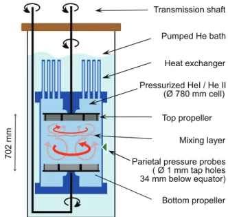
Pumped He bath Pressurized HeI / He II (Ø 780 mm cell) Bottom propeller Heat exchanger 702 mm
Parietal pressure probes ( Ø 1 mm tap holes 34 mm below equator) Transmission shaft
Top propeller Mixing layer
Fig. 1: (Colour online) Schematic of the experiment.
The above equation shows that negative-pressure spikes in a quantum fluid remain markers of high-vorticity re-gions. Superfluid and normal fluid vorticities are probed simultaneouly, and weighted in proportion of the density of each fluid. Note that the low pressure on individual quantum vortices has been invoked to explain the trap-ping of light particles along vortices (see [16,30,31] and references therein).
Experimental set-up. –
The von K´arm´an flow. The von K´arm´an flow used
for this experiment has been extensively described in a dedicated paper [32]. We only recall below its main spec-ifications, see fig. 1.
The liquid helium4
He used in this experiment was se-quentially set to temperatures of 2.4 K, 2.1 K and 1.6 K, that is both above and below the superfluid transition
tem-perature (Tλ ≃ 2.15 K at 3 bars). These three
tempera-tures correspond respectively to superfluid fractions of 0%, 19% and 80% at the pressures of interest (see table 1). The pressurization of the flow prevents the occurrence of cavitation for all flow conditions.
The flow is enclosed in a 780-mm-diameter cylindri-cal vessel and it is mechanicylindri-cally stirred by two co-axial bladed disks of radius R = 360 mm, located 702 mm away, counter-rotating in this work. The 8 blades on each disk are curved, and the direction of rotation is such that the convex side of the blades moves into the fluid. This specific direction is chosen because it results in a stable large-scale circulation between the disks [32].
Such a stirring gives rise to two counter-rotating sub-flows separated by a mixing layer, as depicted in, fig. 1. The (mean) position of this mixing layer is determined by
the relative angular velocities Ωb and Ωt of the bottom
and top disks. For exact counter-rotation (Ωb = Ωt), the mixing layer is located at mid-height. In this study, we set
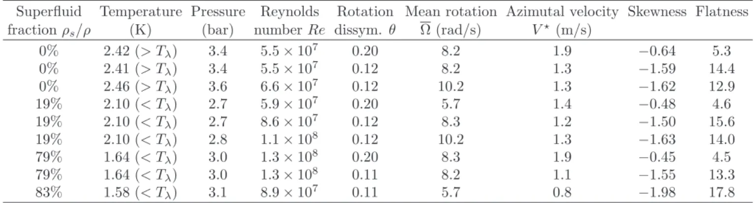
Table 1: Characteristics of the times series.
Superfluid Temperature Pressure Reynolds Rotation Mean rotation Azimutal velocity Skewness Flatness
fraction ρs/ρ (K) (bar) number Re dissym. θ Ω (rad/s) V⋆ (m/s)
0% 2.42 (> Tλ) 3.4 5.5 × 10⁷ 0.20 8.2 1.9 −0.64 5.3 0% 2.41 (> Tλ) 3.4 5.5 × 10⁷ 0.12 8.2 1.3 −1.59 14.4 0% 2.46 (> Tλ) 3.6 6.6 × 10⁷ 0.12 10.2 1.3 −1.62 12.9 19% 2.10 (< Tλ) 2.7 5.9 × 10⁷ 0.20 5.7 1.4 −0.48 4.6 19% 2.10 (< Tλ) 2.7 8.6 × 10⁷ 0.12 8.3 1.2 −1.50 15.6 19% 2.10 (< Tλ) 2.8 1.1 × 10⁸ 0.12 10.2 1.3 −1.63 14.0 79% 1.64 (< Tλ) 3.0 1.3 × 10⁸ 0.20 8.3 1.9 −0.45 4.5 79% 1.64 (< Tλ) 3.0 1.3 × 10⁸ 0.11 8.2 1.1 −1.55 13.3 83% 1.58 (< Tλ) 3.1 8.9 × 10⁷ 0.11 5.7 0.8 −1.98 17.8
Ωb> Ωt, to position the mixing layer above the mid-plane away from the probes which are located 34 mm below this mid-plane. The relative angular velocity of the disks is characterized by
θ = Ωb− Ωt Ωb+ Ωt
. (7)
The parameter θ was set to 11–12% and 20% to probe the flow at two distances from the mixing layer. In classical
von K´arm´an flow, the Reynolds number is often defined as
Re = ρR 2 (Ωb+ Ωt) 2µ = ρR2 Ω µ , (8)
where ρ is the density of the fluid and Ω is the mean
angular velocity. For our purposes, this definition
re-mains a convenient control parameter below the super-fluid transition. Indeed, at large scales, the supersuper-fluid and normal fluid are strongly locked by the mutual coupling force which make them behave as a single fluid of viscosity µ [8,33].
The flow parameters θ and Re used in the present study are given in table 1. We stress that this study is performed
at ultra-large Reynolds number, of order Re ≃ 108 rarely
reached in laboratory conditions. Following [34], the typ-ical Taylor microscale Reynolds number can be assessed
from Re as Rλ≃$(Re) ≃ 10000.
Instrumentation. –
The parietal pressure probes. Fluctuations of parietal
pressure are monitored at two locations, both 34 mm be-low the mid-plane and at 80 mm from each other (mea-sured along the sidewall circumference). At each location, a differential transducer senses the pressure difference be-tween an orifice in the sidewall and a pressure reference.
The pressure reference is low-pass-filtered by an hy-draulic impedance so that it mirrors the static pressure inside the flow, and follows its possible slow drift. From the spectral analysis of the measured pressure fluctuations, this lower cut-off frequency of the probe is estimated to be significantly lower than 100 mHz.
The orifice in the flow sidewall is a square-edge 1-mm-diameter hole, perpendicular to the wall, with an effective
depth of around 20 mm. The membrane of the pressure transducer is mounted at the end of this connecting pipe. The Helmholtz resonance is close to 1 kHz and mechanical vibrations of the transducers are damped using a mechan-ical filter.
In practice, the largest useful frequencies of the mea-sured signal was not limited by the probe itself but by broadband pressure oscillations in the flow, in the hun-dreds of hertz range. Those oscillations were probably originating from the cryogenic system maintaining the ex-periment cold.
Electronics and acquisition. Each piezo-resistive
pres-sure transducer consists in a Wheatstone bridge laying over a deflecting membrane. Each bridge is polarized by a battery-based ∼ 350 mA current source. The bridge output voltage is amplified using a low-noise
instrumen-tation preamplifier (0.6 nV/√Hz, model EPC1-B). A
8th-order linear-phase anti-alias filter at frequency fc (Kemo 1208/20/41LP) is inserted before an 18-bits acquisition board (National Instrument 6289). Acquisitions are
per-formed at sampling frequency 20 kHz (with fc = 6 kHz)
and last between 25 and 45 min, except for a few sam-pled at 1 kHz (with fc = 200 Hz) for practical reasons. All times series are post-processed by a numerical low-pass filter at 160 Hz to avoid possible post-processing artifacts caused by the Helmholtz resonance.
Results. –
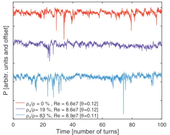
Detection of coherent structures in turbulent superfluid. We first discuss the classical flow regime (ρs/ρ = 0). The red time series plotted in fig. 2 illustrates the recording of several sharp depressions during 100 rotations of the disks. The time axis is scaled by 2π/Ω so that it corresponds to a number of turns of the disks.
Two possible artifacts of the measurements are acoustic noise within the fluid and mechanical noise propagating along the mechanical structure of the experiment. Pres-sure fluctuations were simultaneously recorded from two nearby sensors (as previously done in [24], for example), and were compared. Most depressions are only captured by one probe, which would not be the case if they were
E. Rusaouen et al.
0 20 40 60 80 100
Time [number of turns]
P [ a rb it r. u n it s a n d o ff s e t] ρs/ρ = 0 % , Re = 6.6e7 [θ=0.12] ρs/ρ= 19 %, Re = 8.6e7 [θ=0.12] ρs/ρ= 83 %, Re = 8.9e7 [θ=0.11]
Fig. 2: (Colour online) Pressure time series at 3 temperatures for roughly similar forcing. The superfluid fraction ranges from 0% to 84%. Time on the x-axis is rescaled by the mean rotation time 2π/Ω of the disks. The sharp depressions are interpreted as the signature of vortical coherent structures passing over the pressure tap.
caused by an external noise source. Occasionally, depres-sions are recorded by both probes with mean delays con-sistent with the mean direction of the flow, which confirms that the measured signal corresponds to localized coherent structures carried in the fluid.
Assuming a passive transport of the coherent structures between the two probes, the delay can be interpreted as a “time of flight” and gives the local flow (azimutal) veloc-ity V⋆ using the 8 cm probe separation. It is found in the m · s−1 range, as given in table 1. With V⋆ = 1.6 m · s−1 and taking 160 Hz as the effective noise-free probe dynam-ics, we find a noise-free effective probe resolution of 1 cm but the wavelet analysis of the raw time series (without the 160 Hz low-pass filter) allows to track the signature of the depression nearly up to the ≃ 1 kHz probe resonance frequency, showing that the coherent structures can be at least as thin as 1.6 m · s−1/1 kHz ≃ 2 mm, to be compared with the large scale L of such von K´arm´an flows [28],
L ≃ R/2 ≃ 200 mm, (9)
and to rough estimates of the Taylor and Kolmogorov dis-sipative scales λ and η based on the homogeneous isotropic turbulence equations,
λ ∼ L ·$10/Re⋆≃ 0.2 mm, (10)
η ∼ L/Re⋆3/4≃ 10−3mm, (11)
where we took Re⋆ = LV⋆ρ/µ ≃ 1.4 · 107
. Surely, the flow is neither homogeneous nor isotropic, but these equa-tions can still provide useful orders of magnitude, and show that the present probe is partly resolving the in-ertial range of the turbulent cascade, which extends from ∼ L down to ∼ 10η. -10 -5 0 10-4 10-3 10-2 10-1
P [standard deviation unit]
P ro b a b ili ty d e n s it y ρ s/ρ= 0 %, Re=5.5e7 [θ=0.12] ρ s/ρ= 0 %, Re=6.6e7 [θ=0.12] ρ s/ρ= 19 % Re=5.9e7 [θ=0.20] ρ s/ρ= 19 % Re=8.6e7 [θ=0.12] ρ s/ρ= 19 % Re=1.1e8 [θ=0.12] ρ s/ρ= 79 % Re=1.3e8 [θ=0.20] ρ s/ρ= 79 % Re=1.3e8 [θ=0.11] ρ s/ρ= 83 % Re=8.9e7 [θ=0.11] gaussian (standard deviation=1) ρ
s/ρ= 0 %, Re=5.5e7 [θ=0.20]
Fig. 3: (Colour online) Probability density function (pdf) of the pressure fluctuations normalized to unity standard deviation.
We now address the superfluid regime. Figure 2 illus-trates two typical times series with superfluid fractions of
ρs/ρ = 19% and 83% acquired at Reynolds numbers
sim-ilar to the classical regime (Re = 7.107
± 16%). As in the classical case, sharp depressions are found. No qualitative difference is found between the classical and superfluid regimes when all the acquired time series are scrutinized. To the best of our knowledge, this is the first experimen-tal evidence of coherent structures detected in a turbulent superfluid. We present below a quantitative analysis of the strength, density spatial distribution of those coher-ent structures with respect to their classical counterpart.
Histogram of pressure: density and strength of
coher-ent structures. Figure 3 shows the probability
den-sity functions (pdf) of pressure time series normalized by the standard deviation of their positive pressure fluctua-tions. The pdf shape is compatible with the description
given in classical turbulence literature for von K´arm´an
flows [23,24,26–28]. It can be approximated as
Gaus-sian complemented with a long exponential tail associated to the rare but intense negative pressures spikes associ-ated with the coherent structures. Such skewed pressure pdf have been reported in a number of classical lent flows, for instance in homogeneous isotropic turbu-lence [35,36], along the centerline of pipes [37] and in jets [38]2
. One advantage of the von K´arm´an geometry
over these other flows is the efficient generation of vortex filaments in its mixing layer, and the resulting significant enhancement of the pressure skewness compared to the background skewness resulting from the quadratic veloc-ity dependence of pressure [40].
Whatever the superfluid fraction and Reynolds num-ber, all the pdf corresponding to a given θ are found to collapse, up to our statistical uncertainty. In other words, the density and strength of coherent structures are
2In boundary layers more symmetrical pdf can be found, see,
6e+07 8e+07 1e+08 1.2e+08 1.4e+08 -2.5 -2 -1.5 -1 -0.5 0 Re skewness
6e+07 8e+07 1e+08 1.2e+08 1.4e+08 0 5 10 15 20 Re flatness
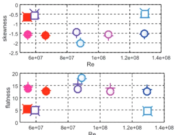
Fig. 4: (Colour online) Upper (lower) plot: skewness (flatness) of pressure fluctuations. The open (full) symbols correspond to measurements in superfluid (in classical liquid helium). The square-shaped (circle-shape) symbols are for a differential ro-tation parameter of θ = 0.2 (θ = 0.11–0.12). The crosses and pluses symbols correspond to the probe-bandwidth check with 53 Hz low-pass filtering (see text).
found independent of the superfluid fraction from 0% up to 83% of superfluid. This is the second important result of this study. When θ is lowered, the mixing layer gets closer to the probes and the density of coherent structures increases. This suggests that the mixing layer is an intense source of coherent structures, both in classical and super-fluid turbulence. The dependence with the distance to the mixing layer can then be understood as the result of the finite lifetime [27] of the vortical coherent structures. This provides an indirect indication that the lifetime of the co-herent structures is similar in the classical and superfluid cases.
The asymmetry and flatness of the pdf can be assessed quantitatively from two statistical quantities: the skew-ness and kurtosis of the pressure fluctuations. They are respectively defined as the centered third and fourth mo-ments of the fluctuations normalized by their standard deviation.
Figure 4 shows the measured skewness and flatness (kurtosis) below and above the superfluid transition tem-perature. The numerical values are given in table 1. Ap-plication of an additional 160 Hz/3 ≃ 53 Hz low-pass filter on the time series does not alter significantly those quanti-ties suggesting that we do not have time resolution issues. For a given value of θ, no Reynolds number dependence
emerges from our measurements when Re ∼ 108is varied
by a factor 2.3, justifying a posteriori that the definition of a Reynolds number below the superfluid transition is not critical in the present study. On the contrary, the dependence of both parameters vs. θ is around a factor 3. Spatial distribution of superfluid coherent structures. To go one step further in the comparison of coherent structures, we now address their relative spatial distri-bution in the classical and superfluid regimes. To this end, we focus on the statistics of time interval δT between two consecutive coherent structures passing by one probe.
0 10 20 30 40
101
102
103
δT [in numbers of turns]
counts
Classical fluid (ρs/ρ=0%), Re = 5.5e7 [θ=0.12] Superfluid ( ρ
s/ρ = 83 %), Re = 8.9e7 [θ=0.11] independent events stat. (1 mean occurence / 11.5 turns)
Fig. 5: (Colour online) Histogram of the intervals between successive coherent structures which are larger than δT . To improve statistical convergence, the statistics from two pres-sure taps (thin lines) have been averaged (thicker line). The dashed line corresponds to the expected dependence of inde-pendent events with a mean separation of 11.5 mean rotations (see text).
We need to choose an arbitrary criterion for identifica-tion of coherent structures. Several criteria have been proposed and studied in the classical turbulence litera-ture, with little incidence in the respective conclusions (e.g., see [24–26,41]). Following [26], we choose a pres-sure threshold at −3 in standard deviation units. Larger thresholds of 4 and 5 were also tested and gave compatible results but with a worse statistical convergence. In fig. 5, the y-axis represents the number of intervals between suc-cessive coherent structures which are larger than δT (x-axis). For the best convergence, the longest time series at temperatures corresponding to 0% and 83% of superfluid have been chosen and the times series from the two probes (thin lines) were averaged together (thick lines).
If coherent structures were fully independent of each other, we would expect a Poisson statistics for the inter-vals p(δT ) ∼ e−δT /τ. By integration, the probability of an interval larger than δT is proportional to τ e−δT /τ. This exponential law accounts reasonably well for the results for intervals δT longer than a characteristic correlation time of ∼ 10 mean rotation periods, in good agreement with the classical turbulence literature [26,41]. A fit gives a mean separation time τ = 11.5 ± 1.5 in units of rotation period. For shorter intervals, the statistics is no longer exponential. This reveals a trend for coherent structures to cluster, which is found similar in the classical and su-perfluid cases. In a frozen turbulence picture, this result means that the spatial distribution of the coherent struc-tures is found similar in classical and quantum flows.
Concluding remarks. – If the pressure probes were
able to resolve individual quantum vortices, dissipative scales or the genuine pressure profile of a vortex bundle, some differences between measurements in a classical and
E. Rusaouen et al.
in a quantum flows would be apparent. Obviously, the resolution of the present probes is not as such, but we showed that it is sufficient to clearly detect the individ-ual coherent structures, from their measured (low-pass-filtered) pressure profile. Thus, the statistics of occurrence and strength of coherent structures could be characterized and we found that they are statistically indistinguishable when measured in a classical flow and with a superfluid fraction of 19% and 79% to 83%. In other words, the microscopic differences in internal structures of classical vorticity filaments and superfluid vortex bundles do not prevent both types of coherent structures from recovering similar macroscopic properties.
Among the perspectives, it would be interesting to
re-late these findings to the unexpected f−5/3 vortex line
spectra [14], which have been interpreted as passive scalar spectra postulating that a large amount of vorticity was localized at small scales and carried by the flow [42,43]. The presence of vortex bundles could support well this interpretation (for an alternative interpretation, see [44]). Another interesting perspective is to explore temperatures around 1.9 K where a singular behavior has been numeri-cally predicted for intermittency [45,46], but not yet evi-denced experimentally [11,47]. A third perspective would be understand the dissipative interaction between the bun-dles of superfluid vortices and the (possibly overlapping) filaments of normal fluid.
∗ ∗ ∗
Financial support from EC Euhit project (WP21) is acknowledged, and special thanks go to its coordinator
E. Bodenschatz for his initiative. We also thank the
members of the SHREK Collaboration, with whom the facility was designed [32], M. Bon Mardion for facility operation, A. Girard for Euhit aspects, P. Diribarne and M. Gibert for support in data-logging flow
param-eters and B. H´ebral for discussions and proof reading.
We warmly acknowledge the help from O. Cadot in un-derstanding better the origins of the skewness of pressure, and the feedback from Y. Tsuji.
REFERENCES
[1] Siggia E. D., J. Fluid Mech., 107 (1981) 375.
[2] She Z.-S., Jackson E. and Orszag S. A., Nature, 344 (1990) 226.
[3] Vincent A. and Meneguzzi M., J. Fluid Mech., 225 (1991) 1.
[4] Douady S., Couder Y. and Brachet M. E., Phys. Rev. Lett., 67 (1991) 983.
[5] Jimenez J. and Wray A. A., J. Fluid Mech., 373 (1998) 255.
[6] Baggaley A. W., Barenghi C. F., Shukurov A. and Sergeev Y. A., EPL, 98 (2012) 26002.
[7] Kivotides D., Phys. Rev. Lett., 96 (2006) 175301. [8] Morris K., Koplik J. and Rouson D. W. I., Phys. Rev.
Lett., 101 (2008) 015301.
[9] Barenghi C. F., Skrbek L. and Sreenivasan K. R., Proc. Natl. Acad. Sci. U.S.A., 111 (2014) 4647.
[10] Barenghi C. F., L’vov V. S. and Roche P.-E., Proc. Natl. Acad. Sci. U.S.A., 111 (2014) 4683.
[11] Maurer J. and Tabeling P., Europhys. Lett., 43 (1998) 29.
[12] Salort J., Baudet C., Castaing B., Chabaud B., Daviaud F., Didelot T., Diribarne P., Dubrulle B., Gagne Y., Gauthier F., Girard A., H´ebral B., Rousset B., Thibault P.and Roche P.-E., Phys. Flu-ids, 22 (2010) 125102.
[13] Salort J., Chabaud B., L´evˆeque E.and Roche P.-E., EPL, 97 (2012) 34006.
[14] Roche P.-E., Diribarne P., Didelot T., Franc¸ais O., Rousseau L. and Willaime H., EPL, 77 (2007) 66002.
[15] Bradley D. I., Fisher S. N., Gu´enault A. M., Haley R. P., O’Sullivan S., Pickett G. R.and Tsepelin V., Phys. Rev. Lett., 101 (2008) 065302.
[16] Bewley G. P., Lathrop D. P. and Sreenivasan K. R., Nature, 441 (2006) 588.
[17] Paoletti M. S., Fisher M. E., Sreenivasan K. R. and Lathrop D. P., Phys. Rev. Lett., 101 (2008) 154501. [18] Van Sciver S., Helium Cryogenics, International
Cryo-genics Monograph Series(Springer) 2012.
[19] Donnelly R. J., Quantized Vortices in Helium-II, Cam-bridge Studies in Low Temperature Physics (Cambridge University Press, Cambridge) 1991.
[20] Bradshaw P. and Koh Y., Phys. Fluids, 24 (1981) 777.
[21] Horne W. C., Smith C. A. and Karamcheti K., Phys. Rev. Lett., 69 (1992) 2602.
[22] Raynal F., Phys. Fluids, 8 (1996) 2242.
[23] Fauve S., Laroche C. and Castaing B., J. Phys. II, 3 (1993) 271.
[24] Cadot O., Douady S. and Couder Y., Phys. Fluids, 7 (1995) 630.
[25] Roux S., Muzy J. and Arneodo A., Eur. Phys. J. B-Condens. Matter Complex Syst., 8 (1999) 301. [26] Chainais P., Abry P. and Pinton J.-F., Phys. Fluids,
11(1999) 3524.
[27] Titon J. H. C. and Cadot O., Phys. Rev. E, 67 (2003) 027301.
[28] Burnishev Y. and Steinberg V., Phys. Fluids, 26 (2014) 055102.
[29] Hills R. N. and Roberts P. H., Arch. Ration. Mech. Anal., 66 (1977) 43.
[30] Sergeev Y. A. and Barenghi C. F., J. Low Temp. Phys., 157 (2009) 429.
[31] Guo W., La Mantia M., Lathrop D. P. and Van Sciver S. W., Proc. Natl. Acad. Sci. U.S.A., 111 (2014) 4653.
[32] Rousset E. A., Rev. Sci. Instrum., 85 (2014) 103908. [33] Roche P.-E., Barenghi C. F. and Leveque E., EPL,
87(2009) 54006.
[34] Mordant N., Pinton J.-F. and Chilla F., J. Phys. II, 7(1997) 1729.
[35] M´etais O.and Lesieur M., J. Fluid Mech., 239 (1992) 157.
[36] Pumir A., Phys. Fluids, 6 (1994) 2071.
[37] Lamballais E., Lesieur M. and M´etais O., Phys. Rev. E, 56 (1997) 6761.
[38] Tsuji Y. and Ishihara T., Phys. Rev. E, 68 (2003) 026309.
[39] Tsuji Y., Fransson J. H. M., Alfredsson P. H. and Johansson A. V., J. Fluid Mech., 585 (2007) 1. [40] Holzer M. and Siggia E., Phys. Fluids A: Fluid Dyn.,
5(1993) 2525.
[41] Abry P., Fauve S., Flandrin P. and Laroche C., J. Phys. II, 4 (1994) 725.
[42] Roche P.-E. and Barenghi C. F., EPL, 81 (2008) 36002.
[43] Salort J., Roche P.-E. and L´evˆeque E., EPL, 94 (2011) 24001.
[44] Nemirovskii S. K., Phys. Rev. B, 86 (2012) 224505.
[45] Bou´e L., L’vov V., Pomyalov A. and Procaccia I., Phys. Rev. Lett., 110 (2013) 014502.
[46] Shukla V. and Pandit R., Phys. Rev. E, 94 (2016) 043101.
[47] Salort J., Chabaud B., L´evˆeque E.and Roche P.-E., J. Phys.: Conf. Ser., 318 (2011) 042014.