HAL Id: halshs-02919697
https://halshs.archives-ouvertes.fr/halshs-02919697
Preprint submitted on 23 Aug 2020HAL is a multi-disciplinary open access
archive for the deposit and dissemination of sci-entific research documents, whether they are pub-lished or not. The documents may come from teaching and research institutions in France or abroad, or from public or private research centers.
L’archive ouverte pluridisciplinaire HAL, est destinée au dépôt et à la diffusion de documents scientifiques de niveau recherche, publiés ou non, émanant des établissements d’enseignement et de recherche français ou étrangers, des laboratoires publics ou privés.
Persistence-Dependent Optimal Policy Rules
Jean-Bernard Chatelain, Kirsten Ralf
To cite this version:
Jean-Bernard Chatelain, Kirsten Ralf. Persistence-Dependent Optimal Policy Rules. 2020. �halshs-02919697�
WORKING PAPER N° 2020 – 49
Persistence-Dependent Optimal Policy Rules
Jean-Bernard Chatelain Kirsten Ralf
JEL Codes: Keywords:
Persistence-Dependent Optimal Policy
Rules
Jean-Bernard Chatelain
Kirsten Ralf
yAugust 22, 2020
Abstract
A policy target (for example in‡ation) may depend on the persistent compo-nent of exogenous shocks, such as the cost-push shock of oil, energy or imported prices. The larger the persistence of these exogenous shocks, the larger the welfare losses and the larger the response of policy instrument to this exogenous shock in a feedback rule, in order to decrease the sensitivity of the policy target to this shock.
JEL classi…cation numbers: C61, C62, E31, E52, E58.
Keywords: Core in‡ation, Imported in‡ation, Optimal Policy, Welfare, Policy rule.
1
Introduction
Ramsey optimal policy theoretically grounds Ashley, Tsang and Verbrugge’s (2020) em-pirical evidence that the Fed funds rate response increases with the persistence of exoge-nous shocks. For example, imported in‡ation or oil prices changes do have a persistent component (Ashley and Tsang (2013))).
Firstly, the optimal response of the policy instrument to persistent shocks increases with the auto-correlation of shocks. Although the central bank cannot control the persis-tence of exogenous shocks, it can control the sensitivity of core in‡ation to these shocks with its policy rule response.
Secondly, optimal policy may even set this sensitivity to zero when responding to non-stationary shocks when the auto-correlation tends to one. This is one explanation among others for the observed smaller order of the dynamics of the policy target (a smaller number of lags) than the order of the dynamics (the number of lags) of the policy instrument. For example, this is the case for US in‡ation (one lag) and Fed funds rate (two lags) for quarterly data from 1982 to 2006.
Thirdly, a non-zero weight in the loss function of the variance of the policy instruments (which respond to persistent exogenous shocks) implies that the value function which evaluates welfare depends on the volatility of persistent exogenous shocks. This occurs even if the loss function has sets a zero weight on the volatility of persistent exogenous shocks.
Paris School of Economics, Université Paris 1 Pantheon Sorbonne, PjSE, 48 Boulevard Jourdan, 75014 Paris. Email: [email protected]
yESCE International Business School, INSEEC U. Research Center, 10 rue Sextius Michel, 75015 Paris, Email: [email protected].
2
Persistence-Dependent Optimal Policy Rule
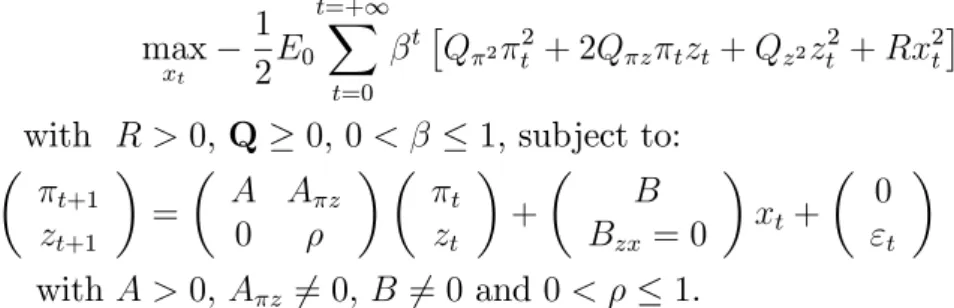
The policy maker’s optimal policy program is:max xt 1 2E0 t=+1X t=0 t Q 2 t2+ 2Q z tzt+ Qz2zt2+ Rx2t
with R > 0, Q 0, 0 < 1, subject to:
t+1 zt+1 = A A z 0 t zt + B Bzx= 0 xt+ 0 "t with A > 0, A z 6= 0, B 6= 0 and 0 < 1.
where Et denotes the expectation operator, t denotes the rate of core in‡ation
be-tween periods t 1and t. The persistent cost-push shock ztmay correspond to oil, energy
or imported in‡ation due to foreign supply or demand shocks. The policy instrument is xt. It may represent the welfare-relevant output gap, i.e. the deviation between (log)
output and its e¢ cient level (Gali (2015)).
The policy maker preferences includes a discount factor and weights Q on the
variance and covariance of in‡ation and of the persistent cost-push shock and R on the variance of the policy instrument. Q is a positive matrix. R is strictly positive.
The cost-push shock follows an autoregressive process of order one (AR(1)), 0 < 1, with identically and independently normally distributed white noise disturbances "t of
variance 2
". The policy maker’s instrument cannot change the persistence of this shock
(Bzx= 0). The full system of core in‡ation and imported in‡ation is of order two.
Our results do not depend on speci…c relations between the parameters ( ; A; A z; B)
of the policy transmission mechanism. They hold for backward-looking models assum-ing in‡ation is predetermined or for Ramsey optimal policy where in‡ation is non-predetermined and optimally anchored by the policy maker. They can be extended to multiple policy targets, multiple persistent shocks and multiple policy instruments using Chatelain and Ralf (2019, 2020) algorithm. In this case, only numerical values are avail-able. Closed form solutions can only be found for order two models with single target, single persistent shock and single policy instrument as follows.
We apply these results on Gali (2015, chapter 5) new-Keynesian Phillips curve (NKPC) transmission mechanism (table 1):
t= xt+ Et t+1+ zt , Et t+1 =
1
t xt
1
zt (1)
Table 1: New-Keynesian Phillips curves parameters and welfare
pref-erences, = 0:99, = 0:1275, " = 6.
Parameters A B A z Q 2 Q z Qz2 R
NKPC 1 1 < 0 1 = A 1 0 0
"
Calibration 0:991 0:12750:99 0:991 1 0 0 0:12756 = 2:125% 0:8
Gali’s (2015) example has a large sensitivity (close to one in absolute value) between
core in‡ation and cost-push shock: A z = 1 = 0:991. One percent change of imported
in‡ation leads to one percent change of core in‡ation (A z = 1 = 1:01). Gali’s
(2015) calibration uses welfare computation for the weight on the variance of the policy
values of optimal policy parameters consistent to an allowed large variance of the policy instrument.
Following Chatelain and Ralf (2019, 2020) algorithm, the optimal policy rule is de…ned by endogenous policy rule parameters: F for the response of the policy instrument to core in‡ation, Fz for the response of the policy instrument to persistent shocks:
xt= F t+ Fzzt (2)
The results of optimal policy are summarized in the following propositions. Proofs are in the appendix.
Proposition 1 Optimal core "intrinsic" in‡ation persistence is controllable by the policy
maker and equal to = A + BF . The optimal response of the policy instrument to policy
target F do not depend on the exogenous persistence ( ) of cost-push shock nor on the sensitivity of core in‡ation to these cost-push variables (A z):
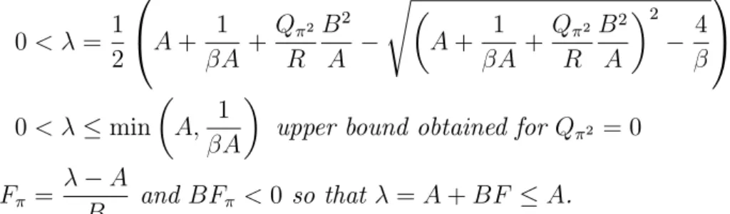
0 < = 1 2 0 @A + 1 A + Q 2 R B2 A s A + 1 A + Q 2 R B2 A 2 4 1 A 0 < min A; 1
A upper bound obtained for Q 2 = 0
F = A
B and BF < 0 so that = A + BF A.
Example 1 For Gali’s (2015) calibration, because the welfare weight on the variance of
the policy instrument in the loss function is implausibly low (R=Q 2 = 2%), this implies a very low persistence of in‡ation ( = 0:4291604) due to an implausibly large negative-feedback response of the policy instrument (F = 4:51) to deviations of in‡ation from its long run target.
The comparison between policy rules which do not react to the persistent exogenous cost-push shocks versus optimal policy rules are presented in …gures 1 to 4 corresponding to the following propositions. They highlight the dependence on the persistence of shocks
( ) of the response of the policy instrument Fz to persistent shocks, of the resulting
sensitivity of the policy target to the cost-push shock A z+ BFz, of the resulting impulse
response functions of in‡ation, of the initial jump of non-predetermined in‡ation 0 and
of welfare W . Welfare is a particular case of Chatelain and Ralf (2020).
Figure 1 to 4: Key parameters functions of imported in‡ation persistence:
1: Sensitivity A z+ BFz = 2: Optimal policy parameter Fz 0.0 0.2 0.4 0.6 0.8 1.0 -1.0 -0.5 0.0 Rho Az+BFz 0.0 0.2 0.4 0.6 0.8 1.0 -8 -6 -4 -2 0 Rho Fz
3: In‡ation initial jump 0 4: Welfare W
0.0 0.2 0.4 0.6 0.8 1.0 0.0 0.5 1.0 Rho Pi0 0.0 0.2 0.4 0.6 0.8 1.0 -100 -50 0 Rho W
Proposition 2 The absolute value of the sensitivity of the policy target to the cost-push shock after policy rule response below the sensitivity before policy intervention jA z+ BFzj <
jA zj. It is a non-linear decreasing function of the persistence of the of the cost-push shock
measured by . It is an a¢ ne function of the sensitivity A z of the policy target to the
persistent shock when the policy instrument does not respond to cost-push shock. We
denote = A z+ BFz = A z+ BFz = A 1 1 A z(1 A ) Q z B2 R One has: jA z+ BFzj < jA zj because BF A = A A < 0
When cost-push shock tends to zero persistence, the sensitivity tends a lower sensitivity than the one obtained for Fz = 0.
lim
!0jA z + BFz( )j = A zA jA zj
When cost-push shock persistence tends to a unit root, the absolute value of the sensitivity of the policy instrument to the cost-push shock reaches its lowest value:
lim !1(A z+ BFz) = A 1 1 A z(1 A ) Q z B2 R
Because 6= 0 and 6= 0, this lowest value is equal to zero for A = 1= (which is a
property of the new-Keynesian Phillips curve) and for a zero weight on the covariance of in‡ation and cost push shock Q z = 0 in the loss function.
persistence = 0:8 of the cost-push shock, because the welfare weight on the variance of the policy instrument in the loss function is extremely low (2%), the large response of the policy instrument to the cost-push shock implies that the sensitivity of the in‡ation to the cost push shock is 13% of what it would have been if the policy instrument would not have responded to the persistent cost-push shock (Fz = 0):
A z+ BFz = (1 ) 1 = 0:4291604 (1 ) 1 0:4291604 0:99 = 0:13 lim !1(A z+ BFz) = 0 because A = 1 and Q z = 0: lim !0jA z + BFzj = j j = 0:429 < 1 = 1:01
Proposition 3 Core in‡ation overall persistence and impulse response function …rstly
depends on its "intrinsic" persistence (controllable root = A + BF ) and secondly depends on the "extrinsic" non-controllable imported in‡ation persistence of the cost push shock, which is itself attenuated by the policy instrument response Fz to the cost-push
shock decreasing the sensitivity of core in‡ation to the cost-push shock A z+ BFz.
Et t A z + ; + = t 0+ t t z0 if 6=
Under the condition A = 1, if the cost-push shock autocorrelation tends to one, the
order of the dynamics of the policy target is reduced to one (single eigenvalue ): lim !1Et t = t 0 if A = 1 and Q z = 0 so that ! 0
Example 3 For Gali’s (2015) calibration, the impulse response function of core in‡ation
is lower when the policy rule responds to imported in‡ation (Fz 6= 0) than when the policy rule does not respond to imported in‡ation (Fz = 0). This is because the sensitivity of
core in‡ation to imported in‡ation is 13% of 1 = 1:01:
Et t = 0:429t 0+ 0:8t 0:429t 0:8 0:429 ( 0:13) z0 lim !1Et t = 0:429 t 0
In the limit case of unit root persistence for the cost push shock ( ! 1) such as a trend in oil price, the sensitivity of in‡ation to the cost push shock (A z+ BFz) tends to
zero, so that in‡ation is an order one process (with single root ) instead of an order two
process depending on two roots ( and of the cost-push shock).
Proposition 4 The policy instrument has a persistence-dependent rule parameter Fz
increasing in absolute value with the persistence of the cost-push shock. It increases in absolute value with the sensitivity A z of the policy target to the cost-push shock:
Fz A z + ; + = A z B = Fz = A z A 1 1 A B Q z A B R 1
The limit are: lim !0jFz( )j = A z A A B > 0 = Fz( = 0) lim !0jFz( )j = 0 if Q 2 = 0 and if = A < 1
The lack of response of the policy instrument when the persistence of the shock tends to zero is obtained only in an irrelevant case where welfare and the policy maker do not weight the volatility of the policy target in the loss function Q 2 = 0 and if in‡ation is stationary for a …xed setting of the policy instrument at its long run equilibrium value ( = A < 1).
Example 4 As seen in …gure 1, for Gali (2015) persistence = 0:8 of the cost-push
shock, because the welfare weight on the variance of the policy instrument in the loss function is extremely low (2%), this allows large variations of the policy instrument with a large response of the policy instrument to the cost-push shock ( 6:86):
Fz = 1 1 1 = 1 0:1275 1 0:4291604 0:99 1 0:4291604 0:99 = 6:86 lim !0jFz( )j = jF j = 4:52 > jFz( = 0)j = 0 and lim!1jFz( )j = 7:84
Proposition 5 If core in‡ation 0 is non-predetermined, in Ramsey optimal policy, it is
optimally anchored on the policy instrument which is itself anchored on the predetermined cost-push shock. The …rst order conditions sets the marginal value of the loss function with respect to in‡ation at the initial date (itself equal to it costate variable, the Lagrange
multiplier 0) equal to zero. Initial core in‡ation 0 increases with imported in‡ation
persistence . @L @ 0 = 0 = 2 (P 2 0+ Pzz0) = 0) 0 = P 21P z z0 0 A z + ; + = 1 1 A z + Q z Q 2 (1 A) lim !0 0 = A z Q z Q 2 (1 A)
Example 5 As seen in …gure 3, with Gali’s (2015) calibration ( = 0:8):
0 = 1 = 0:4291604 1 0:4291604 0:99 = 0:64 lim !0 0 = = 0:42274, lim!1 0 = 1 = 0:73
Proposition 6 Welfare: Even if households and/or Central Bank preferences set a zero
weight on the covariance between core in‡ation and cost-push shock (Q z = 0) and the
variance of cost-push shock (Qzz = 0), the variance of the policy instrument depends on
this variance. Therefore, the optimal value of welfare depends on the covariance of core in‡ation and of the cost-push shock (P z 6= 0) and of the variance of the cost-push shock
(Pzz 6= 0). Both weights (P z; Pzz) increases with the persistence of the cost-push shock
(the opposite of the optimal value of the loss function) decreases in a non-linear fashion
with the persistence of imported in‡ation and with the sensitivity of core in‡ation to
imported in‡ation A z with no response of the policy instrument to the cost-push shock.
Welfare can be computed for a given initial predetermined in‡ation 0 as follows. For
non-predetermined in‡ation, we take into account the optimal initial anchor of in‡ation for the welfare of Ramsey optimal policy, using 0 = P 21P zz0:
W A z; = P z P 2z0 z0 P 2 P z P z Pz2 P z P 2z0 z0 = Pz2 P2 z P 2 z02 > 0
Example 6 For welfare dependence on the persistence of the cost-push shock, with Gali’s
(2015) calibration with = 0:8 (…gure 4):
W z2 0 = (1 )2(1 2) = 0:4291604 (1 0:99 0:4291604 )2 1 1 0:99 2 = 2:688 lim !0 W z2 0 = = 0:429, lim !1 W z2 0 = (1 )2(1 ) = 130
3
Conclusion
Optimal policy facing persistent exogenous cost-push shock, for example, imported in‡a-tion or de‡ain‡a-tion due to oil or energy shocks implies a dependence to the persistence of the cost-push shock …rstly of the policy instrument in the policy rule, secondly of the policy target persistence and of its impulse responses function through a change of its sensitivity to the cost push shock and of the initial jump of in‡ation and thirdly of welfare.
References
[1] Chatelain, J.B. and Ralf, K. (2019). A Simple Algorithm for Solving Ramsey Optimal Policy with Exogenous Forcing Variables. Economics Bulletin. 39(1). pp. 2429-2440. [2] Chatelain, J.B. and Ralf, K. (2020). The Welfare of Ramsey Optimal Policy Facing
Auto-regressive shocks. Economics Bulletin. 40(2), pp. 1797-1803.
[3] Ashley, R, Tsang K. P. and Verbrugge R. (2020). “A New Look at Historical Monetary Policy and the Great In‡ation through the Lens of a Persistence-Dependent Policy Rule”. Oxford Economic Papers. 72(3). pp.692-671.
[4] Ashley R. and Tsang K. P. (2013). “International Evidence on the Oil Price-Macroeconomy Relationship: Does Persistence Matter?” Working Paper, Virginia Tech.
[5] Gali J. (2015). Monetary Policy, In‡ation, and the Business Cycle, (2nd edition) Princeton University Press.
4
Appendix
Stable subspace of the Hamiltonian system
Following Chatelain and Ralf (2020), we form the Lagrangian by attaching a sequence
of Lagrange multipliers t+1
t+1 and t+1 t+1to the sequence of constraints of the policy
transmission mechanism: L = t=+1X t=0 t 2 4 1 2Q 2 2 t + Q z tzt+ 21Qz2zt2+1 2Rx 2 t + t+1(A t+ Bxt+ A zzt t+1) + t+1( zt zt+1) 3 5 The …rst order necessary conditions are:
@L @xt = Rxt+ B t+1= 0 ) xt = B R t+1 or t+1 = R Bxt @L @ t = Q 2 t+ Q zzt+ A t+1 t= 0 @L @zt = Q z tt+ Qz2zt+ A z t+1+ vt+1 vt= 0
The Hamiltonian system is: 0 B B @ 1 0 BR2 0 0 1 0 0 0 0 A 0 0 0 A z 1 C C A 0 B B @ t+1 zt+1 t+1 t+1 1 C C A = 0 B B @ A A z 0 0 0 0 0 Q 2 Q z 1 0 Qz Qz2 0 1 1 C C A 0 B B @ t zt t t 1 C C A
We seek the elements of the value function (welfare) matrix: P 2, P z and Pz2, which are the unknown parameters of eigenvectors of the stable subspace of the Hamiltonian
system: 0 B B @ t zt t t 1 C C A = 0 B B @ 1 0 0 0 0 1 0 0 P 2 P z 0 0 Pz Pz2 0 0 1 C C A 0 B B @ t zt t t 1 C C A It follows: 0 B B @ B2 RP 2 + 1 B2 RP z 0 1 AP 2 AP z P z+ A zP 2 Pz2 + A zP z 1 C C A zt+1t+1 = 0 B B @ A A z 0 P 2 Q 2 P z Q z P z Q z Pz2 Qz2 1 C C A ztt
We eliminate zt+1 by zt. Solving the model amounts to use the following three key
equations for …nding the three unknown parameters P 2, P z and Pz2 of the welfare matrix: 0 @ 1 + B2 RP 2 AP 2 P z+ A zP 2 1 A ( t+1) = 0 @ A A z B2 RP z P 2 Q 2 (1 A) P z Q z P z Q z (1 2) Pz2 Qz2 A zP z 1 A t zt (3)
The …rst terms of the three equations implies three formulas for the intrinsic
persis-tence of the policy target, = A + BF :
= A + BF = A 1 + BR2P 2 = P 2 Q 2 A P 2 = P z Q z P z + A zP 2 .
The second terms of the three equations implies three formulas for the sensitivity of
the policy target to the persistent shock, = A z+ BF z, with F z = BA z.
= A z B2 R P z 1 + RB2P 2 = (1 A) P z Q z AP 2 = (1 2) P z2 Qz2 A zP z P z+ A zP 2 .
Proof of proposition 1. Compute the optimal root = A + BF , a …rst
ele-ment of the welfare matrixP 2 (proposition 5a) and the policy rule parameter
F :
The …rst term of each of the three equation has the same value:
= A 1 + BR2P 2 = P 2 Q 2 A P 2 = P z Q z P z+ A zP 2
Using the …rst equality:
1 + B 2 R P 2 = A , P 2 = R B2 A > 0 Using the second equality:
P 2 Q 2 = A P 2 , P 2 =
Q 2
1 A
Using the …rst and second equality leads to a characteristic polynomial for solving :
1 + B 2 R P 2 A = 0 1 + B 2 R Q 2 1 A A = 0 2 A + 1 A + B2Q 2 AR + 1 = 0
Optimal persistence is the stable root of this characteristic polynomial:
0 < = 1 2 0 @A + 1 A + Q 2 R B2 A s A + 1 A + Q 2 R B2 A 2 4 1 A 0 < min A; 1 A for Q 2 = 0
F = A
B and BF < 0 so that = A + BF A.
Proof of proposition 5b: Second element of the welfare matrix P z
We use the third equality for the …rst term:
= A 1 + BR2P 2 = P 2 Q 2 A P 2 = P z Q z P z+ A zP 2
P z is an increasing function of the two characteristics of the forcing variable A z and
: P z Q z = P z+ A zP 2 ) P z = A zP 2 + Q z 1 With: P 2 = R B2 A = Q 2 1 A
P z can be written as a function of :
P z(A z; ) = 1 1 A z R B2 A + Q z P z(A z; ) = 1 1 A z R B2 (A ) + Q z or P z(A z; ) = 1 1 A zQ 21 A + Q z
Proof of proposition 2: Compute the sensitivity = A z+ BFz:
One has: = A z B2 RP z A = (1 A ) P z Q z AP 2 = (1 2) P z2 Qz2 A zP z P z+ A zP 2 .
In the …rst equality, substitute P z and the denominator by A= leads to:
= A A z 1 B2 R A z R B2 (A ) + Q z = A A z 1 1 (A ) Q z B2 R 1 = A A z 1 A 1 Q z B2 R 1
Proof of example 2: For Gali’s example: Q z = 0 and A = A z = 1=
= 1 1 1
1 = (1 )1
Proof of proposition 3: The impulse response function of in‡ation The following result can be found using at least three methods:
t= t 0
(A z+ BFz) z0
+ t(A z + BFz) z0
(a) Solve the sum of two geometric sequences or geometric progressions using the
homogeneous solution related to the geometric sequence with common ratio and a
particular solution proportional to the forcing variable following a geometric sequence with common ratio ;
(b) compute the power of the matrix A z+ BFz
0 using its Jordan
decompo-sition;
(c) prove it by mathematical induction.
Proof of proposition 4: Policy rule parameter Fz:
Fz = A z B = A z B A A A 1 Q z B R A A Fz = A z AB A 1 Q z B R A A Fz = A z A 1 1 A B Q z A B R 1
Proof of example 4: For Gali’s example: Q z = 0 and A = A z = 1=
Fz =
1 1
1
Proof of proposition 5c: Optimal jump of in‡ation 0:
The …rst order conditions sets the marginal value of the loss function with respect to in‡ation at the initial date (itself equal to it costate variable, the Lagrange multiplier 0)
equal to zero. @L @ 0 = 0 = 2 (P 2 0+ Pzz0) = 0 ) 0 A z + ; + = P z P 2 z0 One has: P z P 2 = 1 P 2 Q z+ A z P 2 1 and P 2 = Q 2 1 A P z P 2 = 1 1 A z + Q z Q 2 (1 A)
Proof of proposition 6: Welfare parameter Pz2
shock determines Pz2: = A A z B2 R P z = (1 A ) P z Q z AP 2 = (1 2) P z2 Qz2 A zP z P z+ A zP 2
The third equality leads to:
1 2 Pz2 = Qz2 + (A z + ) P z + A zP 2 with: P z = 1 1 A z Q 2 1 A + Q z and P 2 = Q 2 1 A A z+ = A z+ (1 A ) P z Q z A P 2 so that: P 2 P z P z Pz2 = Q 2 1 A Q z 1 Q z 1 Qz2 1 2 ! + 0 1 1 A z P 2 1 1 A z P 2 1 1 2 ((A z+ ) P z+ A zP 2)
Proof of welfare, example 6 (Gali): Computation of Pz2:
1 2 Pz2 = Qz2 + ( P z+ A zP 2) + A z P z with: P z = 1 1 1 and P 2 = 1 1 = (1 ) 1 , Qz2 = 0, A z = 1 One has: 1 2 Pz2 = 1 (1 ) 1 1 1 1 1 1 1 1 2 Pz2 = 1 1 1 2 1 1 Pz2 = 1 1 (1 )2 1 2 1 2 so that: P= 1 1 1 1 1 1 1 1 1 1 (1 )2 1 2 1 2 ! = 1:7518055 1:1389181 1:1389181 3:4285107
For welfare dependence on the persistence of the cost-push shock, with Gali’s (2015) calibration: Pz2 = 1 1 (1 )2 1 2 1 2 = 3:4285 P2 z P 2 = 1 1 2 (1 )2
Welfare has this form: W z2 0 = Pz2 + P2 z P 2 = 1 1 (1 )2 1 2 1 2 W z2 0 = 1 1 (1 )2 1 1 2 W z2 0 = (1 )2 1 1 2 = 0:4291604 (1 0:99 0:4291604)2 1 1 0:99 2 W z2 0 = 0:4291604 (1 0:99 0:8 0:4291604)2 1 1 0:99 0:82 = 2:688 QED.
SCILAB Code for numerical solutions: beta1=0.99; eps=6; kappa=0.1275; rho=0.8; Qpi=1; Qz=0 ; Qzpi=0; R=kappa/eps;
A1=[1/beta1 -1/beta1 ; 0 rho] ; A=sqrt(beta1)*A1;
B1=[-kappa/beta1 ; 0]; B=sqrt(beta1)*B1;
Q=[Qpi Qzpi ;Qzpi Qz ]; Big=sysdiag(Q,R); [w,wp]=fullrf(Big); C1=wp(:,1:2); D12=wp(:,3:$); M=syslin(’d’,A,B,C1,D12); [Fy,Py]=lqr(M) A1+B1*Fy -inv(Py(1,1))*Py(1,2) Py(2,2)-Py(1,2)*inv(Py(1,1))*Py(1,2)