HAL Id: hal-02928408
https://hal.archives-ouvertes.fr/hal-02928408
Submitted on 7 Sep 2020HAL is a multi-disciplinary open access
archive for the deposit and dissemination of sci-entific research documents, whether they are pub-lished or not. The documents may come from teaching and research institutions in France or abroad, or from public or private research centers.
L’archive ouverte pluridisciplinaire HAL, est destinée au dépôt et à la diffusion de documents scientifiques de niveau recherche, publiés ou non, émanant des établissements d’enseignement et de recherche français ou étrangers, des laboratoires publics ou privés.
Hawkes point processes based inference applied to
seismic data analysis
Loubna Ben Allal, Antoine Lejay, Radu S. Stoica
To cite this version:
Loubna Ben Allal, Antoine Lejay, Radu S. Stoica. Hawkes point processes based inference applied to seismic data analysis. 2020 RING MEETING, Sep 2020, Nancy, France. �hal-02928408�
Hawkes point processes based inference applied to seismic data analysis
Loubna Ben Allal1, A. Lejay2, and R. S. Stoica21Mines Nancy/ F-54000 Nancy
2Université de Lorraine, CNRS, Inria, IECL, F-54000 Nancy, France
September 2020
Abstract
The occurrences of earthquakes can be regarded as a point process. The arrivals of these earthquakes are, however not independent. Large earthquakes can trigger aftershocks. We say that the process is self-exciting. Hawkes processes are widely used self-exciting processes to model such phenomena. In this article, we apply these models with an exponential decay function to seismic data and show their relevance.
Introduction
Hawkes processes are self-excited counting processes: each event increases the rate of future arrivals over time. This is the case with aftershocks of earthquakes; an earthquake increases the geographical tension in the region and can cause a second earthquake (Ogata, 1988). This paper presents properties, simulation algorithms, and inference methods to fit a one-dimensional Hawkes process to seismic data. The modeling of Hawkes processes in terms of the conditional intensity and its simulation using a thinning algorithm is presented in Section 1. Statistical inference procedures are discussed in Section 2, while Section 3 is dedicated to practical applications on simulated and real earthquake data from Guadeloupe over 2004-2005. Finally, conclusions and perspectives are depicted.
1
Modeling of Hawkes processes and simulation
This part introduces basic notions regarding Hawkes processes. For this presentation, we have fol-lowed Laub, Taimre, and Pollett (2015). For more details, the interested reader may consult Daley and Vere-Jones (2003).
1.1 Modeling in terms of conditional intensity
Definition 1. We consider a counting process (𝑁 (𝑡), 𝑡 > 0), defined as the number of events that occurred up to time 𝑡, with associated history (𝐻(𝑡), 𝑡 > 0) of arrivals, and conditional intensity defined as
𝜆*(𝑡) = lim
ℎ→0
E(𝑁 (𝑡 + ℎ) − 𝑁 (𝑡)|𝐻(𝑡))
ℎ . (1)
A Hawkes process is such a counting process defined by a constant 𝜆 > 0, called background intensity and a function 𝜇 : [0, +∞) → [0, +∞), called excitation function, such that
𝜆*(𝑡) = 𝜆 + ∫︁ 𝑡 0 𝜇(𝑡 − 𝑠) d𝑁 (𝑠) = 𝜆 + 𝑛 ∑︁ 𝑖=1 𝜇(𝑡 − 𝑡𝑖),
Let us recall that the choice of the intensity in (1) means that for all 𝑡, ℎ > 0,
P(𝑁 (𝑡 + ℎ) − 𝑁 (𝑡) = 0|𝐻(𝑡)) = 1 − 𝜆*(𝑡)ℎ + o(ℎ),
P(𝑁 (𝑡 + ℎ) − 𝑁 (𝑡) = 1|𝐻(𝑡)) = 𝜆*(𝑡)ℎ + o(ℎ),
P(𝑁 (𝑡 + ℎ) − 𝑁 (𝑡) = 𝑛|𝐻(𝑡)) = o(ℎ) for any 𝑛 > 1.
Each arrival increases the intensity of future arrivals which makes the process self-exciting. The form of this self-excitation depends on the excitation function 𝜇. In this article, we use the exponential decay function 𝜇(𝑡) = 𝛼 exp(−𝛽𝑡). In this case, more recent events have a higher influence on the process. Each event instantaneously increases 𝜆* by 𝛼 and the influence of this event decreases over time at rate 𝛽.
Theorem 1. For the process to be well defined it is necessary that
𝑛 = ∫︁ ∞
0
𝜇(𝑠) d𝑠 < 1.
A proof of this result can be found in Laub et al. (2015).
If 𝑛 ≥ 1, the model explodes. For an exponential decay excitation function we should respect the condition 𝛼 < 𝛽.
1.2 Simulation with thinning algorithm
To simulate a Hawkes process we use the thinning algorithm (see e.g., Chen, 2016): Similarly to the generation of an inhomogeneous Poisson process. Knowing 𝑡1, 𝑡2, ..., 𝑡𝑘, 𝜆* is deterministic on [𝑡𝑘, 𝑡𝑘+1],
so we can see the generation of the point 𝑡𝑘+1 as the generation of the first point of an inhomogeneous
Poisson process using a rejection procedure. We use Ogata’s modified algorithm (Ogata, 1981, p.25, Algorithm 2).
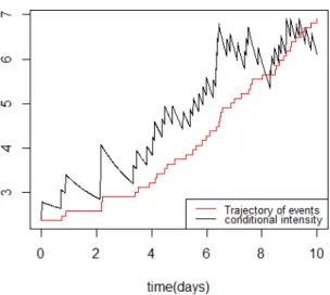
Figure 1 shows the conditional intensity curve of a simulated Hawkes process with parameters 𝛼 = 0.6, 𝛽 = 0.8 and 𝜆 = 2 on a period 𝑇 = 10, superimposed on the event curve. We observe that each jump in the intensity corresponds to the arrival of a new event, and after some time, the events occur more frequently than at the beginning.
2
Inference and model validation
The Hawkes process has 3 parameters to estimate. We present a maximum likelihood procedure.
2.1 Likelihood function
Theorem 2 (Hawkes process likelihood). Let 𝑁 be a Hawkes process with a conditional intensity 𝜆* and let {𝑡1, . . . , 𝑡𝑘} be the arrival times on [0, 𝑇 ]. The likelihood 𝐿 of the process is
𝐿 = 𝑘 ∏︁ 𝑖=1 𝜆*(𝑡𝑖) exp (︂ − ∫︁ 𝑇 0 𝜆*(𝑢) d𝑢 )︂ .
A proof of this expression can be found in Daley and Vere-Jones (2003)[Section 7.2].
In the case of an exponential decay function 𝜇(𝑡) = 𝛼 exp(−𝛽𝑡), the log-likelihood function is in the form ℓ = log 𝐿 = 𝑘 ∑︁ 𝑖=1 ln ⎛ ⎝𝜆 + 𝛼 𝑖−1 ∑︁ 𝑗=1 exp(−𝛽(𝑡𝑖− 𝑡𝑗)) ⎞ ⎠− 𝜆𝑡𝑘+ 𝛼 𝛽 𝑘 ∑︁ 𝑖=1 exp (−𝛽(𝑡𝑘− 𝑡𝑖)).
Hawkes processes applied to seismic data Ben Allal et al.
Figure 1: The conditional intensity curve of a simulated Hawkes process with parameters 𝛼 = 0.6, 𝛽 = 0.8 and 𝜆 = 2, superimposed on the event curve.
2.2 Parameter estimation
To estimate the model parameters, we need to maximize the (log-)likelihood function. It is a max-imization problem with linear constraints. In the case of exponential decay excitation function, the objective function is asymptotically concave. In R, we use the optimization method ConstrOptim. It transforms the problem into a constraint free problem using a logarithmic barrier and then solves it by using the constraint free optimization function Optim of R.
2.3 Model validation: residual analysis
In this section, we present an approach to check the goodness of fit of a Hawkes process to some arrival times of a point process. This approach is called residual analysis (See Daley & Vere-Jones, 2003, Theorem 7.4.I.).
Theorem 3. Let {𝑡1, 𝑡2, . . . } be the arrival times of a point process 𝑁 . We define the cumulative
inten-sity Λ as Λ(𝑡) = ∫︀0𝑡𝜆*(𝑠) d𝑠. The residuals sequence {𝜏1, 𝜏2, . . . } = {Λ(𝑡1), Λ(𝑡2), . . . } is a realisation
of a unit rate Poisson process if and only if 𝑁 is a Hawkes process with conditional intensity 𝜆*. Given the arrivals of a counting process and the estimated parameters using the maximum likelihood procedure, we check if the residuals of this model form a unit rate Poisson process. In practice, we use the envelope test, where we plot the envelope of a unit rate Poisson process and we superimpose several samples of Hawkes processes with the estimated parameters, generated by the thinning algorithm. These samples have to be within the envelope, this test also allows us to have a vision of the average behavior of Hawkes processes with the same parameters. We can also check if the inter-arrivals of the residuals are exponential variables with unit rate, using a Kolmogorov-Smirnov test. Another possible test is to check whether the martingale residuals, defined as 𝑅(𝑡) = 𝑁 (𝑡) −∫︀𝑡
0𝜆
*(𝑢)𝑑𝑢, are close to 0
(Daley & Vere-Jones, 2003, Lemma 7.2.V), they actually represent the error between the model and the data accumulated over time.
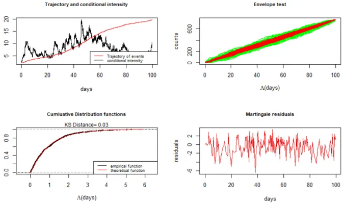
Figure 2: Inference procedures on synthetic data: Conditional intensity curve superimposed on event curve, envelope test ( the green curves correspond to unit rate Poisson processes and the red curves correspond to the residuals of the simulated Hawkes processes),
Kolmogorov-Smirnov test and martingale residuals.
3
Application to synthetic and real data
3.1 Simulated data
First, in order to verify the previously presented results, we have performed statistical inference on the data given by a simulated process.
The obtained estimation results are ˆ
𝜆 = 2.06, ˆ𝛼 = 0.61, ˆ𝛽 = 0.81.
The real values are 𝜆 = 2, 𝛼 = 0.6 and 𝛽 = 0.8, so the estimated values are close to the real ones. If the unit of time is days, then the value 𝜆 = 2 means that every day, 2 events that are not aftershocks arrive.
Figure 2 makes a synthetic presentation of the implemented inference procedures.
The envelope test consists of the residuals of 100 simulated Hawkes processes with parameters ˆ𝛼, ˆ
𝛽 and ˆ𝜆 in the time interval [0, 𝑇 ] with 𝑇 = 100 days. These residuals are all within the envelope, which confirms that they are unit rate Poisson processes. The martingale residuals oscillate around 0, therefore the error between the model and the data accumulated over time is small.
Concerning the Kolmogorov-Smirnov test of the inter-arrivals of the residuals. The test returns a p-value equal to 0.65. This value is high so we cannot reject the hypothesis of having a sequence that follows an exponential law of unit rate. The Kolmogorov-Smirnov test plot shows the distribution function of the empirical data and that of the exponential distribution of unit rate. The two functions are very close, and the Kolmogorov-Smirnov distance is equal to 0.03 which is a small value. Therefore all of these tests do not reject the null hypothesis, that the residuals form a unit rate Poisson process, so the process is a Hawkes process with a conditional intensity whose parameters are 𝛼, 𝛽 and 𝜆.
Hawkes processes applied to seismic data Ben Allal et al.
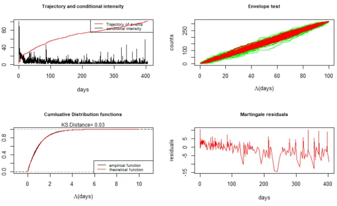
Figure 3: Inference procedures on seismic data: Conditional intensity, envelope test, Kolmogorov-Smirnov test and martingale residuals.
3.2 Inference for the seismic data from Guadeloupe
As an application of what we have presented, we use the earthquake data in Guadeloupe during the years 2004 - 2005 obtained by RING Team. We test if the Hawkes process provides us with a suitable model for this seismic sequence, consisting of the main earthquakes that occurred after November 21, 2004. The earthquakes’ arrival times were in seconds and we converted them into days, to guarantee numerical stability for the maximum likelihood optimization.
We found the following estimated values ˆ
𝜆 = 1.76, ˆ𝛼 = 3.44, ˆ𝛽 = 5.06.
In this case ˆ𝜆 = 1.76 means that every 1/1.76 days, an event that is not an aftershock arrives.
Figure 2 makes a synthetic presentation of the implemented inference procedures. The residuals of the envelope test are all within the envelope, which confirms that they are unit rate Poisson processes. The martingale residuals oscillate around 0 and they move slightly away from 0 around day 110. Concerning the Kolmogorov-Smirnov test plot, it shows the distribution function of the empirical data and that of the exponential distribution of unit rate. The two functions are very close, and the Kolmogorov-Smirnov distance is equal to 0.03 which is a small value. However, the p-value of the test is equal to 0.02. These results encourage us to pursue the modeling work based on Hawkes point processes by using also the information provided by the magnitudes.
4
Conclusions and perspectives
This paper introduced the Hawkes point process and applied it to simulated and real seismic data. A simulation algorithm based on a thinning procedure was also presented together with a parameter estimation procedure. Statistical tests using residual analysis were also provided to verify the estimation quality and to validate the obtained model.
The conditional intensity of the proposed model was built using an exponential decay excitation. The results obtained on real data showed that Hawkes processes are indeed a mathematical tool that is interesting for such type of data. In order to improve the quality of the results several points should be mentioned: using other models than exponential, extending the mathematical framework to the marked and spatial cases (See Ogata, 1988, 1998).
Acknowledgments
The authors would like to acknowledge Corentin Gouache and the RING team from GeoRessources for kindly providing the seismic data.
References
Chen, Y. (2016). Thinning algorithms for simulating point processes. Florida State University, Talla-hassee, FL.
Daley, D. J., & Vere-Jones, D. (2003). An introduction to the theory of point processes, volume I: Elementary theory and methods (2nd ed.). Springer Science & Business Media.
Laub, P. J., Taimre, T., & Pollett, P. K. (2015). Hawkes processes. arXiv preprint arXiv:1507.02822 . Ogata, Y. (1981). On Lewis’ simulation method for point processes. IEEE transactions on information
theory , 27 (1), 23–31.
Ogata, Y. (1988). Statistical models for earthquake occurrences and residual analysis for point pro-cesses. Journal of the American Statistical association, 83 (401), 9–27.
Ogata, Y. (1998). Space-time point-process models for earthquake occurrences. Annals of the Institute of Statistical Mathematics, 50 (2), 379–402.
Hawkes processes applied to seismic data Ben Allal et al.