HAL Id: hal-01038118
https://hal.archives-ouvertes.fr/hal-01038118
Submitted on 29 Sep 2020HAL is a multi-disciplinary open access
archive for the deposit and dissemination of sci-entific research documents, whether they are pub-lished or not. The documents may come from teaching and research institutions in France or abroad, or from public or private research centers.
L’archive ouverte pluridisciplinaire HAL, est destinée au dépôt et à la diffusion de documents scientifiques de niveau recherche, publiés ou non, émanant des établissements d’enseignement et de recherche français ou étrangers, des laboratoires publics ou privés.
Sliding window proper orthogonal decomposition:
Application to linear and nonlinear modal identification
Simon Clément, Sergio Bellizzi, Bruno Cochelin, Guillaume Ricciardi
To cite this version:
Simon Clément, Sergio Bellizzi, Bruno Cochelin, Guillaume Ricciardi. Sliding window proper orthog-onal decomposition: Application to linear and nonlinear modal identification. Journal of Sound and Vibration, Elsevier, 2014, 333 (21), pp.5312-5323. �10.1016/j.jsv.2014.05.035�. �hal-01038118�
Sliding Window Proper Orthogonal Decomposition :
application to linear and nonlinear modal identification
Simon Clement
∗,∗∗, Sergio Bellizzi
∗∗, Bruno Cochelin
∗∗and Guillaume Ricciardi
∗ ∗CEA Cadarache DEN/DTN/STCP/LHC,
Saint-Paul-Lez-Durance, 13108 Cedex, France
∗∗LMA, CNRS, UPR 7051, Centrale Marseille,
Aix-Marseille Univ, Marseille Cedex 20, France
Abstract
The Proper Orthogonal Decomposition (POD) method is a tool well adapted to analyse vec-tor signals whereas Continuous Gabor Transform (CGT) is suitable for scalar signal with multi-frequency components. In this paper, a method named Sliding Window Proper Orthogonal De-composition (SWPOD) combining POD and CGT to analyse Multi-Degrees-Of-Freedom (MDOF) vibration system responses is presented. SWPOD gives access to the evolution of the coherent spacial structures and their frequency components versus time. The method is of principal in-terest in the case of swept-sine excitation of linear or nonlinear systems to access the resonance frequencies, mode shapes and modal damping ratios. A procedure is proposed to extract the lin-ear and non-linlin-ear normal modes of weakly damped MDOF mechanical systems and illustrated using numerical examples.
1
Introduction
The study of complex vibrating systems with numerous degrees of freedom containing nonlinearities is still a major challenge today. The well-known theory of linear modal analysis is limited in under-standing the practical behavior of real systems, especially when nonlinearities have dominant effects on their behavior. A large variety of methods which are able to deal with nonlinearities have been proposed to characterize and/or identify systems. Time domain approaches, frequency domain ap-proaches, time-frequency apap-proaches, modal approaches have been considered. Moreover, the theory of nonlinear normal modes is promising, but not yet applicable to complex practical systems.
Time-frequency (or wavelet) analysis is a powerful signal processing tool to study signals with time-dependent frequency content. It has been used to characterize and identify mechanical systems. For example, modal analysis of linear mechanical systems based on wavelet transform has been performed using output-only free time responses[1][2][3], and under ambient excitation[4]. These approaches are based on the notion of ridges and skeletons introduced for the continuous wavelet transform of scalar
signals and differ with the choice of wavelet families. Variants from the use of skeleton can be found in [5], where a wavelet-based formula similar to the logarithmic decrement formula has been introduced to estimate damping. Some approaches have been extended to characterize nonlinear mechanical systems (see [2]). Specific methods have also been developed. In [6][7] for example, Continuous Gabor Transform (CGT), a time-frequency transform, is used to estimate the nonlinear normal modes of weakly damped nonlinear systems from free responses. Common to all these methods based on wavelet or time-frequency transform is that they are generally applied independently to each component of the response extracting the localized frequency content for each of them. It is a local method in the space domain.
On the other side, the Proper Orthogonal Decomposition (POD) method is a global approach characterizing spatial coherent structures. It has now emerged as a structural dynamics analysing tool for systems with a high number of Degrees Of Freedom (DOF). The physical interpretation of the Proper Orthogonal Modes (POMs) (the coherent structures) was investigated by several authors [8, 9, 10, 11] with the links between the POMs and the linear normal modes highlighted. In the case of lightly damped linear systems harmonically excited by an external force, it was shown [8] that a single POM captures all the energy and when the excitation frequency is near a resonance frequency, this POM is a linear normal mode of the system. However, in the case of a nonlinear system, the energy can be shared between several POMs and the results of a POD applied to the entire signal can be difficult to interpret as the physical characteristics of the system. For instance, the application of the POD to a nonlinear system excited at different discrete frequencies was investigated by Kerschen et al. [12], showing the appearance of a second energetic POM at frequencies where the nonlinearities of the structure are effective and a modal behavior depending strongly on the excitation frequency.
To analyse data involving complex evolution in time, frequency and space, it is thus relevant to combine POD and time-frequency transform. This combination is at the heart of the Sliding Window POD (SWPOD) method, which gives the evolution of the coherent structures of the data as well as their frequency components versus time. This ambivalent ability can be used to analyse complex simulated or experimental data, with the main structural and frequential characteristics of the signals extracted. The method can also be used to identify the resonance frequencies, mode shapes and damping ratios of a linear system, or to investigate the nonlinear normal modes (NNM) of a nonlinear system. Note that time-frequency transform and POD have already been combined in the context of noise reduction (see [13]), but the POD is applied to the time-frequency transform of a scalar signal and spacial dimension is not present. A method recently developed called Dynamic Mode Decomposition, when applied to experimental data, also gives a set of modes evolving with time, but with a different approach using the Koopman operator [14].
This paper is organized as follows. In Section 2, CGT and POD are first briefly recalled, followed by the description of the SWPOD method including numerical implementation. Section 3 is dedicated to the description of the nonlinear mechanical model used to show the potentiality of the method when applied to the responses obtained under linear swept sine excitation. Responses associated to low and high excitation levels are considered in Section 4 and section 5 respectively. In both cases, the mechanical interpretation of the results obtained with SWPOD is discussed, giving access to the modal parameters in linear (low excitation levels) and nonlinear cases (high excitation levels).
2
Presentation of the SWPOD method
2.1
The Continuous Gabor transform
Continuous Gabor Transform (CGT) of a scalar signal s(t) can be defined from the transform : Gs(τ, f ) =
Z +∞
−∞
s(t)g(t − τ) e−j 2πf (t−τ )
dt (∈ C), (1)
where g(t) is a scalar (real or complex) function named window function but also mother wavelet (this is an abuse of notation) and g denotes the complex conjugate of g. Several types of window functions can be used, such as Hamming, Hanning, Blackman windows, in which cases the signal is truncated and the Gabor transform is called Short Time Fourier Transform (STFT).
Gabor proposed to use Gaussian functions (g(t) = e− t2
2σ2 where σ > 0) as window functions, which
assure the most efficient utilization of the information as shown in [21]. In terms of windowing, σ controls the effective width of the windowing. CGT extracts both time and frequency information from a signal, by applying windows sliding in time (realizing the time localization) before applying the Fourier transform. CGT can be used to capture the time evolution of the frequency content of the signal.
It is important to remember that the CGT can be inverted with the formula s(t) = 1 2πkgk2 Z +∞ −∞ Z +∞ −∞ Gs(τ, f )g(t − τ)ej 2πf (t−τ )dτ df, (2) where kgk2 =R+∞ −∞ |g(t)| 2dt.
2.2
The Proper Orthogonal Decomposition
Let us consider a vector signal S(t) (with N components) for t ∈ R. Without loss of generality, we assume that all components have zero mean values, with respect to the mean operator (or time average, < . >=R+∞
−∞(.)dt). The POD gives the most characteristic vectors Φ representing the evolution of the
vector signal S(t). These vectors can be found by maximizing the time average of the scalar product of the two vectors Φ and S(t):
Maximize < |S(t)TΦ|2 > with ΦTΦ = 1. (3)
The vectors which yield the maximum are solutions of the eigenvalue problem:
RΦ = λΦ with R =< S(t)S(t)T > . (4)
Let λ1 ≥ λ2· · · ≥ λN be the ordered eigenvalues, then the associated N orthonormal vectors Φi can
be used as a basis to expand S(t) as
S(t) =
N
X
i=1
Φipλiηi(t), (5)
where the scalar signals ηi(t) are defined as ηi(t) = ΦTi S(t)/
√
λi and satisfy the orthogonal property
coherent structures. The ηi(t) called Proper Orthogonal Components (POCs) are their normalized
time evolutions representing the dynamics of the signal. The reals λi are the Proper Orthogonal
Values (POVs) defining the energy captured by each POM.
Among the numerous applications of the POD stands reduced order modelling, which uses its ability to reduce the number of POMs necessary to represent the signal from N to Nr if the following
condition is satisfied: Nr X i=1 λi > 99% N X i=1 λi. (6)
This characteristic of the POD allows analysing complex data with a high number of components and in the case of structural dynamics, systems with numerous degrees of freedom.
Finally, as mentioned in the introduction, it was shown in [8] that for a lightly damped system harmonically excited, only one POM captures all the energy of the system. Observing the sharing of energy between POMs can thus be a way to detect the presence of high damping or nonlinearities for harmonically excited systems.
2.3
The proposed method
In order to analyse a vector signal S(t) and capture its spatial evolution as well as its frequency content, POD and CGT can be combined, giving the Sliding Window POD (SWPOD) method.
The window function is first applied to the vector signal S(t) giving the windowed vector signal Sτ
(t) = S(t)g(t − τ). (7)
Next, the windowed vector signal is expanded using the POD as Sτ(t) = N X i=1 Φτ ipλτiη τ i(t). (8)
Note that it is possible to reduce the number of terms in the expansion from N to Nτ, with a criterion
of the typePNτ
i=1λτi ≥ 0.99
PN
i=1λτi. Finally the Gabor transform of S(t) results in the sliding window
POD form GS(τ, f ) = Z +∞ −∞ N X i=1 Φτipλτiητi(t)e −j 2πf (t−τ ) dt, = N X i=1 ΦτipλτiG˜i(τ, f ), (9) where ˜Gi(τ, f ) = R+∞ −∞ η τ i(t)e −j 2πf (t−τ ) dt.
For each time τ , the sliding window POD form (9) gives access for i = 1, · · · , N to • the localized POMs, Φτ
i, which characterize the coherent structures associated to the vector
signal localized around the time τ ; • the localized POVs, λτ
• the localized POCs, ητ
i(t), and their frequency content, ˜Gi(τ, f ).
As well as for the Gabor transform, an inverse formula to (9) is also valid and reads as S(t) = 1 2π||g||2 N X i=1 Z +∞ −∞ Φτ ipλτi Z +∞ −∞ ˆ Gi(τ, f )g(t − τ)ej 2πf (t−τ )df dτ. (10)
2.4
Practical application of the SWPOD
We will assume in what follows that the vector signal S(t) is sampled at the sampling frequency fs
(respecting the Nyquist theorem) and acquired on [0, T ] at P sampled times tp = p/fsfor p = 1, · · · , P
and T = tP. We will also assume that P is a power of two (for the optimization of the Fast Fourier
Transform (FFT)).
A N × P matrix S is thus formed, in which the terms Sn(tp) give the component n of S(t) at the
time tp as S = S1(t1) S1(t2) . . . S1(tP) S2(t1) S2(t2) . . . S2(tP) ... ... . .. ... SN(t1) SN(t2) . . . SN(tP) . (11)
The window function g(t) is sampled with the same sampling frequency and, for each time tp, a
N × P matrix Wp is formed as Wp = g(t1− tp) . . . g(−t1) g(0) g(t1) . . . g(tP − tp) .. . ... ... ... ... ... ... g(t1− tp) . . . g(−t1) g(0) g(t1) . . . g(tP − tp) . (12)
The windowed vector signal around the time tp is obtained as
Sp = S ◦ Wp (13)
where ◦ denotes the Hadamard (or term to term) product. The POD can then be performed directly through a singular value decomposition, as shown in [8], leading to the matrix decomposition :
Sp = UpΣpVpT (14)
where Up and Vp are orthogonal and Σp is diagonal. The columns of Up are the localized POMs Φpi.
The diagonal terms of Σp are the square roots of the localized POVs, σip =pλ p
i. The columns of V p
are the sampled localized normalized POCs, ηip(t). The frequency content ˜Gi(tp, f ) is deduced from
the FFT of ηip(t) at the discrete frequencies fk= kfs/P .
The evolution of the most energetic localized POM with respect to time tp is characterized in
terms of energy by the time-energy plot (tp, λp1), in terms of coherent structure by the time-space plot
(tp, Φp1) and in terms of frequency content by the time-frequency plot (tp, ˜G1(tp, fk)). The second most
performed for all the localized modes contributing to the dynamics of the signal and selected with a criterion of the type PNp
i=1λ p i ≥ 0.99 PN i=1λ p i.
Although the temporal length of the window function as represented by Eq. (12) is T , its effective length Te depends on the bandwidth of the window g(t) and contains a number of samples Pe = Tefs.
Te has an influence on the resolution of the analysis in time and frequency and the choice of Te depends
on the properties of the signal to analyse (changes in dynamic and frequency content). Consider a signal containing temporal events at least distant from Tevent and characteristic frequencies separated
by a minimum of Fevent. Tehas to be short enough to separate the temporal events, giving the condition
Te < Tevent. Moreover, the frequency resolution of the analysis is given by δf = fs/Pe = 1/Te and
has to be inferior to Fevent , leading to the second condition Te > 1/Fevent. When gaussian window
functions are used, Te can be estimated as Te= 6 σ.
Finally, in practical applications, the SWPOD method can be performed at a reduced number Pr
of time steps instead of P , giving the localized parameters λτ
i, Φτi and ηiτ(t) at Pr regularly spread
times τ .
3
Mechanical system under study
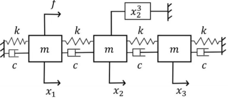
The system considered in this paper is shown in Fig. 1. It is a 3-DOF spring-mass oscillator with linear springs and dashpots (light damping) having both end points related to the ground. The central mass is also connected to the ground with a cubic spring. The system is excited by applying a force on the first mass.
Figure 1: The nonlinear studied system.
The equations of motion reads as :
M ¨X + C ˙X + KX + g(X)V = f (t)B, (15)
with X = (x1, x2, x3)T, V = (0, 1, 0)T, g(X) = x32, B = (1, 0, 0)T and the following mass and stiffness
matrices M = m 0 0 0 m 0 0 0 m , K = 2k −k 0 −k 2k −k 0 −k 2k . (16)
The resonance frequencies of the underlying linear system are given by ω1 =
q
(2 −√2)k/m, ω2 =
p2k/m and ω3 =
q
(2 +√2)k/m with their corresponding linear normal modes Ψ1 = (1/
√
Ψ2 = (1, 0, −1)T and Ψ3 = (−1/
√
2, 1, −1/√2)T. Proportional damping is considered by taking
C = 2ξ1
ω1K, with ξ1(> 0) fixing the damping ratio of the first linear mode.
Considering the modal matrix Ψ = [Ψ1Ψ2Ψ3], the equations of motion can be reduced to :
MΨQ + C¨ ΨQ + K˙ ΨQ + g(ΨQ)ΨTV = f (t)ΨTB, (17) with Q = (q1, q2, q3)T, X = ΨQ, CΨ = 2ξω1 1KΨ and MΨ = 2m 0 0 0 2m 0 0 0 2m , KΨ = 2(2 −√2)k 0 0 0 4k 0 0 0 2(2 +√2)k . (18)
Assuming that m = 1 kg and k = 500 m/N, the natural frequencies of the underlying linear system are f0
1 = 2.72 Hz, f20 = 5.03 Hz and f30 = 6.58 Hz. At low excitation level, characteristic frequencies
are separated by a minimum of Fevent = 1.5 Hz.
In this study, a linear swept sine is used for the excitation f (t) under the form : f (t) = F sin(ϕ(t)) with ϕ(t) = 1 2 2π(fmax− fmin) Tsweep t2+ 2πf min t + ϕ0, (19)
where F is a constant amplitude, Tsweep the time to go from the minimum frequency fmin to the
maximum fmax and ϕ0 the phase at the origin, which is chosen equal to zero. More information on
systems excited by swept sines can be found in references [19] and [20].
In our case, we will perform tests with an excitation frequency varying from fmin = 0.05 Hz to
fmax= 10. Hz over Tsweep= 400 s. At low excitation level, temporal events are at least separated by
Tevent =
FeventTsweep
fmax− fmin ≈ 30 s.
(20) The equations of motion (15) have been solved numerically using the Newmark method with a sampling frequency fs = 200 Hz and zero initial conditions. The signal is produced on [0, T ] with
T = Tsweep corresponding to P = Tsweepfs sampled times. Then, the SWPOD method is applied to the
vector signal S(t) = (x1(t), x2(t), x3(t))T which characterizes the time evolution of the displacements
of the three masses.
Finally, the effective length of the windows Te is defined with σ = 20/6 corresponding to Te ≈ 20
s satisfying Te > 1/Fevent and Te< Tevent.
In the following two sections, the results obtained with SWPOD method at respectively low and high excitation levels are discussed.
4
Low excitation levels (linear behavior)
Two damping ratios are considered in this section, with the excitation level F = 10 N. The behavior of the system is expected to be linear.
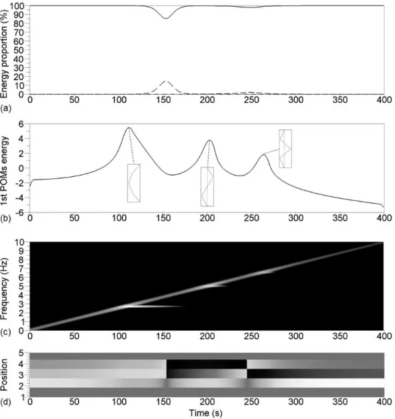
Figure 2: SWPOD analysis of a test with ξ1 = 0.5% and F = 10 N. (a) Proportion of energy captured
by the first 3 POMs λτ 1/
P3
i=1λτi (solid line), λτ2/
P3
i=1λτi (dashed) and λτ1/
P3
i=1λτi (dotted). (b)
Logarithmic representation of the energy captured by the first POM ln(λτ
1). (c) Time-frequency
representation of the first POCs multiplied by the POVs λτ
1Gˆ1(τ, f ). (d) Time evolution of the first
POM with its two extremities : white (black) for high (low) displacements, the extremities giving the color associated to a zero value.
4.1
Case with moderate damping
The first test was carried out with the damping ratio ξ1 = 0.5% on the first mode of the underlying
linear system. Fig. 2 shows the results obtained with the SWPOD. The analysis was performed at Pr = 400 time steps.
The proportions of energy captured by the first three localized POMs are given in Fig. 2(a), showing that the first localized POM is largely dominant and captures more than 99% of the total energy during
most of the test. However, a strong energy sharing between the first two POMs can be observed around 150 s.
The localized POV λτ
1, which characterizes the energy captured by the first localized POM, is given
in Fig. 2(b) (time-energy plot) in logarithmic scale. Three local maxima appear at τ1 = 112 s, τ2 = 203
s and τ3 = 264 s for which the associated localized POM Φτ1i are shown. These shapes are very close
to the normal modes of the underlying linear system. The product λτ
1G˜1(τ, f ) is shown in a time-frequency plot in Fig. 2(c), characterizing the frequency
evolution of the first localized POM. The main frequency content (the oblique line) of the signal follows the linear sweep, with small horizontal lines around 2.73 Hz after 110 s, 5.04 Hz after 200 s and 6.57 Hz after 260 s.
Finally, the time evolution of the shape of the first localized POM (the time-space plot) is given in Fig. 2(d), showing that the system vibrates successively in accordance with the first, second and third normal modes of the underlying linear system.
4.2
Case with low damping
In order to bring a better understanding of the results obtained above and show the ability of the method to deal with complex data, a second test was carried out, reducing the damping ratio ξ1 from
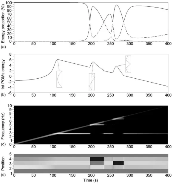
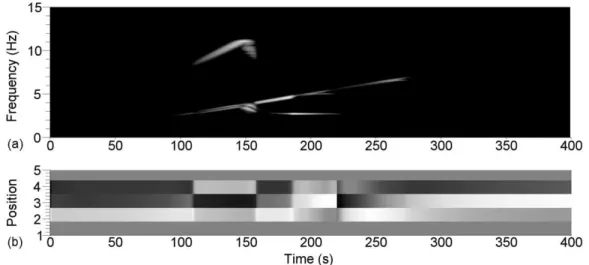
0.5% to 0.1%. The results are reported in Fig. 3. Considering the high sharing of energy between localized POMs and the higher complexity of the behavior of the system, it is interesting to observe the evolution of the second and third localized POMs, reported in Fig. 4 in terms of time-frequency plot and time-space plot.
As shown in Fig. 3(a), the reduction of the damping strongly modifies the sharing of energy between localized POMs. The first energy sharing previously observed with ξ1 = 0.5% at τ = 150 s disappeared
and more complex energy sharings appear. In Fig. 3(b), the local maxima of energy are detected at the same times τ1 = 112 s, τ2 = 203 s and τ3 = 264 s, for which the associated localized POMs are
again very close to the linear normal modes of the system.
The time-frequency plot (see Fig. 3(c)) shows that the horizontal frequency lines, which are initiated passing the resonance frequencies of the underlying linear system, persist on larger time intervals. At the times where two horizontal frequency lines are present (between τ = 200 s and τ = 300 s), the energy captured by the first POM is localized around one of these frequencies, alternating between the frequency lines.
The time-frequency plots of the second and third localized POMs are given in Fig. 4(a,c). The energy is localized in time intervals where energy sharings are observed (Fig. 3(a)). The time-frequency plots have the same structure as the time-frequency plot of the first localized POM, with the oblique frequency line corresponding to the linear sweep component and the horizontal frequency lines initiated at the resonance frequencies of the underlying linear system. Alternances between the horizontal frequency lines (and the oblique line) can also be observed, opposite to the ones of the first POM.
During the time intervals where horizontal frequency lines persist, the time-energy plot (see Fig. 3(b)) shows a linear decrease of energy, with a change of slope when the previous alternances appear. These slopes are strongly linked to the modal parameters of the system and will be used in the next section to identify the damping of the linear normal modes.
The time-space plots (Fig. 3(d) and Fig. 4(b,d)) show that the contribution of the horizontal frequency lines to the vibration of the system are in accordance with the associated normal modes of
Figure 3: Results for a test with ξ1 = 0.1% and F = 10 N. (a) Proportion of energy captured by the
first (solid line), second (dashed) and third (dotted) POMs. (b) Energy captured by the first POM. (c) Time-frequency representation of the first POC multiplied by the POV λτ
1Gˆ1(τ, f ). (d) Time evolution
of the first POM Φτ 1.
the underlying linear system.
Global observations on the results were given above. In the next section, an in-depth analysis of the results will be presented, with the interpretation of the energy sharing detailed and the identification of the modal dampings, frequencies and mode shapes.
Figure 4: Results for the second and third POMs of a test with ξ1 = 0.1% and F = 10 N. (a)
Time-frequency representation of the second POC multiplied by the POV λτ
2Gˆ2(τ, f ). (b) Time evolution
of the second POM Φτ
2. (c) Time-frequency representation of the third POC multiplied by the POV
λτ
3Gˆ3(τ, f ). (d) Time evolution of the third POM Φτ3.
4.3
Physical interpretation of SWPOD at low excitation level
From results discussed in [20], an analytic solution of Eq. (17) (neglecting the nonlinear terms) can be written for each modal component qi(t) as
qi(t) = |Qi(t)| sin(ϕ(t) − αi(t)) (21)
with ϕ(t) defined by Eq. (19) and Qi(t) = |Qi(t)| e −j αi(t)
a complex function (not given here). The amplitude Qi(t) has a maximum located a bit after the passing of the swept sine through the excitation
frequency ωi, which characterizes the resonance of the system. After this maximum, a low-frequency
oscillation of the amplitude |Qi(t)| occurs, which can be interpreted as the superposition of the two
parts of the oscillation: free oscillations at the natural frequency, initiated during the passage of the resonance, and forced oscillations with variable excitation frequency [20]. This interpretation agrees with the results shown in Figs. 2(c) and 3(c) where the oblique frequency lines correspond to forced
oscillations with variable excitation frequency, following the swept sine, and the horizontal frequency lines correspond to free oscillations at the natural frequencies of the system.
The energy sharing in Fig. 2(a) thus comes from the transition between the free oscillation of the first mode and the oscillation following the sweep, whereas the sharings of energy in Fig. 3(a) appear because of the simultaneous free oscillations of several modes. The sudden changes of shape present in the time-space plots Fig. 2(d), Fig. 3(d) and Fig. 4(b,d) appear at these transitions, when the energy sharing is maximum.
The test at ξ1 = 0.1% (Fig. 3) can then be detailed as follows. After the first resonance of the
system at τ1 = 112 s, the most energetic localized POM is the first linear mode of the system during
most of the time, as shown in Fig. 3(d), because of its low damping. The first POM takes the form of the second and third linear normal modes around their resonances at τ2 = 203 s and τ3 = 264
s. These two modes decrease faster than the first one because of their higher dampings, leading to alternances between the three linear normal modes as most energetic POM. Moreover, the different slopes observed in Fig. 3(b) associated to the decay of the three linear normal modes are directly linked to the damping ratio of the modes, as shown below.
The identification of the linear normal modes of the system in term of resonance frequencies and modes shapes can be achieved through SWPOD. The local maxima of the time-energy plot of the first localized POM (which corresponds to maximum of |Qi(t)|) characterize the resonance motions of the
system, giving access to the resonance frequencies and mode shapes. If the local maximum occurs at τi,
the mode shape is then estimated by Φτi
1 and the resonance frequency by arg maxf λ τi
1G˜1(τi, f ). Using
Fig. 2 and Fig. 3, the estimation of the resonance frequencies give 2.73 Hz, 5.04 Hz and 6.57 Hz. and the mode shapes Φτ1
1 = (0.70, 1, 0.71)T, Φ τ2
1 = (1, 0, −1)T for both tests, with Φ τ3
1 = (0.74, −1, 0.69)T
when ξ1 = 0.5% and Φτ13 = (0.73, −1, 0.70)T when ξ1 = 0.1%. These results are very close to the
theoretical linear normal modes of the system, with a slight asymmetry for the third mode.
The damping ratios can also be obtained by focusing on the horizontal frequency lines. They cor-respond to the free oscillations at the natural frequency ωi, initiated during the passage of a resonance
at the time τi. The associated modal motion can then be approximated by :
qi(t) = qi0e −ξiωi(t−τi) cos( q 1 − ξ2 iωi(t − τi) + αi0), (22)
where qi0 and αi0 are real constants imposed when the free motion is initiated. In Eq. (22), the
damping term has been commonly replaced by ci
2m = 2ξiωi. Assuming that in the neighborhood of the
passage of the resonance, the windowed vector signal is reduced to Sτ(t) = Φ
iqiτ(t) where qτ i(t) = qi0e −(t−τ )2 2σ2 e−ξiωi(t−τi)cos( q 1 − ξ2 iωi(t − τi) + αi0), (23)
SWPOD method gives only one localized POM Ψτ
1 = Φi with the associated locatized POV
λτ1 = qi0 Z T 0 e−(t−τ )2 σ2 e−2ξiωitcos2( q 1 − ξ2 iωit + αi0)dt. (24)
Through a change of variables and trigonometric decompositions, Eq. (24) can be written : λτ 1 = e −2ξiωiτ (c0 + c1cos(2 q 1 − ξ2 iωiτ + αi0) + c2sin(2 q 1 − ξ2 iωiτ + αi0)), (25)
where c1 and c2 are constant, small compared to the constant c0. The POV λτ1 can then be considered
as proportional to e−2ξiωiτ
αi = −2ξiωi in the time-energy plot. This property can then be used to identify the modal damping
of the system.
In Fig. 2(b), the slope present after the first local maximum corresponds to the exponential decay of the first mode (see the associated horizontal frequency line Fig. 2(c)). This slope has been estimated using a linear regression giving α1 = −0.166 and used to estimate the associated damping ratio, thus
obtaining the value ξ1 = α1/(2ω1) = 0.486, which is very close to the theoretical one ξ1 = 0.5. In
Fig. 3(b), the slopes present after the three local maxima correspond to the exponential decay of the three modes. These slopes have been estimated respectively as α1 = −0.034, α2 = −0.117 and
α3 = −0.199 and used to estimate the associated damping ratios giving ξ1 = α1/(2ω1) = 0.099%,
ξ2 = α2/(2ω2) = 0.185% and ξ3 = α3/(2ω3) = 0.241%. These values are very close to the theoretical
values ξ1 = 0.1%, ξ2 = 0.185% and ξ3 = 0.242%.
The analysis method proposed is thus able to identify the modal damping of a linear system if the sweep used is fast enough, in addition to identifying its modes and resonance frequencies.
5
High excitation levels (nonlinear behavior)
A moderate damping ratio ξ1 = 0.5% is considered in this section, with high excitation levels. The
behavior of the system is expected to be nonlinear.
5.1
Analysis of a simulated test with a nonlinear behavior
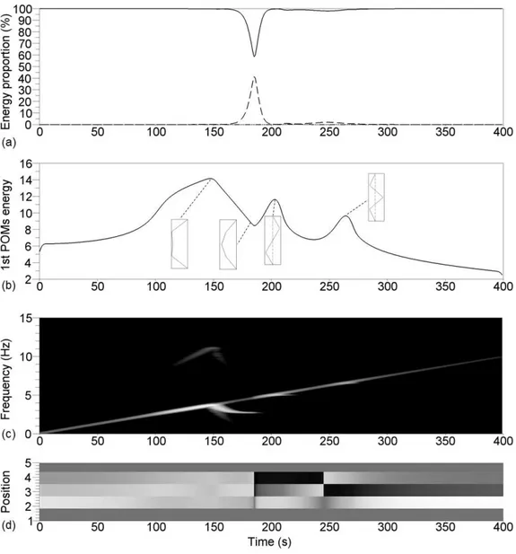
A test was carried out at high excitation level F = 500 N. The results obtained by the SWPOD method are reported in Fig. 5 and Fig. 6.
The proportions of energy captured by the three localized POMs are given in Fig. 5(a), showing results similar to the low amplitude case, with one dominant localized POM during most of the test. From Fig. 5(b), three resonance motions are now detected at τ1 = 147 s, τ2 = 203 s and
τ3 = 264 s, giving the resonance frequencies 3.66 Hz, 5.04 Hz and 6.57 Hz for which the associated
localized POMs Φτ1
1 = (1, 0.94, 1)T, Φτ12 = (1, 0, −1)T and Φτ13 = (0.74, −1, 0.69)T are shown. The
first resonance motion has been translated with respect to the low excitation case (see Fig. 2(b)). The associated resonance frequency is thus higher than the linear one and the associated shape now differs significantly from the first normal mode of the underlying linear system. This result is in accordance with the hardening effect of the nonlinear term. The second resonance motion is not affected by the nonlinearity, because of its position on one of the nodes of the mode. The third resonance motion seems also not affected by the nonlinearity but can be impacted by increasing the excitation amplitude. In the next section, the resonance motions will be investigated in the framework of the nonlinear normal modes (NNM) of the associated autonomous undamped system in terms of frequency and mode shape.
The time-frequency plot (Fig. 5(c)) contains an oblique line for the sweep, as before, but on passing the first resonance motion, a curved frequency line is observed which decreases up to the first resonance frequency of the underlying linear system. As in the low excitation case (linear behavior) this curved line characterizes the free motion initiated passing the first resonance of the system. During this free motion, the decrease of the frequency is now coupled to the variation of the mode shape as shown in Fig. 5(c) for τ ∈ [147, 173]. The two limit mode shapes are shown in Fig. 5(b). The last one corresponds to the mode shape of the first mode of the underlying linear system.
Figure 5: Results for a test with ξ1 = 0.5% and F = 500 N. (a) Proportion of energy captured by the
first (solid line), second (dashed) and third (dotted) POMs. (b) Energy captured by the first POM. (c) Time-frequency representation of the first POC multiplied by the POV λτ
1Gˆ1(τ, f ). (d) Time evolution
of the first POM Φτ 1
It is interesting to note that the decay of the free response is also linear (see Fig. 5(b)). The slope value is α1 = −0.164, which is the same as for the low excitation case (α1 = −0.165 in the linear case),
showing that the first nonlinear mode decays with the same speed as the linear mode, not impacted by the frequency-amplitude dependence. Hence the sharing of energy between the two first localized POMs (see Fig. 5(a)) is here again a transient effect coming from the simultaneous decay of the first resonance and the vibration following the swept sine.
The time-frequency plot (Fig. 5(c)) also shows odd harmonics due to the nonlinear behavior of the system, which is mostly captured by the second POM, as shown in Fig. 6(b).
Figure 6: Results of the sliding window POD analysis for the second POMs for a test with ξ1 = 0.5%
and F = 500 N. (a) Time-frequency representation of the second POC ˆG2(τ, f ). (b) Time evolution
of the second POM Φτ 2.
5.2
Physical interpretation of SWPOD at high excitation levels
The previous analysis was repeated for 33 excitation levels F from 10. N to 10000. N. For each level, the resonance motions were identifed (τi) and characterized as described in Section 4.3 in terms
of frequency (arg maxfλ τi
1G˜1(τi, f )) and mode shape (Φτ1i). The results are reported in Fig. 7 in
a frequency-maximum displacement plot where for each component, the maximum displacement is estimated from Eq. (8) (reduced to the first term) and τ = τi. The results are compared to the NNM
of the associated autonomous undamped system, defined as a familly of periodic orbits and calculated using the harmonic balance method (HBM) and the so-called Asymptotic Numerical Method (ANM) [23]. The NNMs were computed using the software ManLab [22]. With the HBM method the number of harmonics H has to be chosen carefully. All the numerical results were obtained using H =9. It was checked that all the curves were only very slightly modified by increasing H from 9 to 11. Only the first and third NNMs were computed, since the second NNM coincides with the second normal mode of the associated autonomous undamped system and would be represented in Fig. 7 by vertical lines at f0
2 = 5.03 Hz as observed with the SWPOD method.
SWPOD analysis correctly reproduces the third NNM, as well as the first NNM provided that the excitation amplitude remains relatively low. A few mode shapes obtained in this domain of validity are given in Fig. 7, with their corresponding excitation amplitudes. Considering the first NNM, differences appear indeed only at high excitation level (high displacement and frequency values, where the higher harmonic terms have an impact on the displacement of the second mass). The SWPOD, with the proposed identification method, can thus identify a NNM of a system as long as the first harmonic remains dominant i.e as long as the NNM can be considered as a similar NNM [8], i.e as long as the NNM can be captured by the first localized POM in the expansion (8). However, a way to increase the accuracy of the identification of the NNMs is under study, which combines the higher localized POMs obtained around the resonances to take into account the higher harmonics of vibration.
Figure 7: Frequency-maximum displacement plot: displacements of the first and second masses versus the associated resonance frequencies obtained from the simulated tests analysed with SWPOD (plus signs, full line) and the HBM (circles, dashed line) for the first (left) and third (right) NNMs. The shapes obtained at resonance are given for a few excitation amplitudes.
excitation amplitudes from response data alone.
6
Conclusion
An analysis method called Sliding Window POD (SWPOD), combining Proper Orthogonal Decom-position and Continuous Gabor Transform, was proposed. This method can be applied to various types of multivariate data, from experimental or simulated tests. The principal interest of the method is to give a compact representation of both structural and frequential information versus time. The theoretical formulation of the method was posed, then its practical application was detailed. The method was then applied to simulated tests of a lightly damped, nonlinear three-masses system forced following a linear swept sine. Two cases were thoroughly studied : one at low excitation level, and one at high excitation levels.
The simulated tests at low excitation level have shown that the application of the SWPOD to the simulated displacements allows the identification of the resonance frequencies, mode shapes and damping ratios of the underlying linear system. The SWPOD method also showed the ability to separate the forced vibration of the system following the swept sine and its free vibration, which appear on passing its resonances.
The simulated tests at high excitation levels have shown that the method is able to identify the nonlinear normal modes (NNM) of the system in terms of resonance frequencies and mode shapes, for moderate excitation amplitudes. The application of the method, in this paper, was focused on the analysis of structural dynamics, but various applications of the method could be done in different
fields of research.
References
[1] Ruzzene, M., Fasana, A., Garibaldi, L., Piombo, B., Natural frequencies and damping identifica-tion using wavelet transform: Applicaidentifica-tion to real data, Mechanical Systems and Signal Processing 11(2) (1997), 207-218.
[2] Argoul, P., Le, T.P., Instantaneous indicators of structural behaviour based on the continuous Cauchy wavelet transform, Mechanical Systems and Signal Processing 17 (2003), 243-250. [3] Erlicher, S., Argoul, P., Modal identification of linear non-proportionally damped systems by
wavelet transform Mechanical Systems and Signal Processing 21 (2007), 1386-1421.
[4] Le, T.P., Paultre, P. Modal identification based on continuous wavelet transform and ambient excitation tests, Journal of Sound and Vibration 331(2012), 2023-2037
[5] Lamarque, C.-H., Pernot, S., Cuer, A., Damping identification in multi-degree-of-freedom systems via a wavelet-logarithmic decrement-Part 1: Theory, Journal of Sound and Vibration 235(3) (2000), 361-374.
[6] Bellizzi, S., Guillemain P., Kronland-Martinet, R., Identification of coupled non-linear modes from free vibration using time-frequency representations, Journal of Sound and Vibration 232(2) (2001), 191-213.
[7] Camillacci, R.,Ferguson, N.S., White, P.R. Simulation and experimental validation of modal analysis for non-linear symmetric systems, Mechanical Systems and Signal Processing 19 (2005), 21-41.
[8] Kerschen, G., Golinval, J.C., Physical interpretation of the proper orthogonal modes using the singular value decomposition, Journal of Sound and Vibration 249 (2002), 849-865.
[9] Bellizzi, S., Sampaio, R., POMs analysis of randomly vibrating systems obtained from Karhunen-Love expansion, Journal of Sound and Vibration 297 (2006), 774-793.
[10] Han, S., Feeny, B., Application of proper orthogonal decomposition to structural vibration anal-ysis, Mechanical Systems and Signal Processing 17 (2003), 989-1001.
[11] Ricciardi, G., Bellizzi, S., Collard, B., Cochelin, B., Row of fuel assemblies analysis under seismic loading: Modelling and experimental validation, Nuclear Engineering and Design 239, Issue 12 (2009), 2692-2704.
[12] Kerschen, G., Golinval, J.C., Feeny, B., Vakakis, A.F., Bergman, L.A., The Method of Proper Orthogonal Decomposition for Dynamical Characterization and Order Reduction of Mechanical Systems : An Overview, Nonlinear Dynamics 41 (2005), 147-169.
[13] Hassanpour, H., A time-frequency approach for noise reduction, Digital Signal Processing 18 (2008), 728-738.
[14] Kutz, J. N., Data-Driven Modeling & Scientific Computation. Methods for Complex Systems & Big Data, Oxford, New York, 2013.
[15] Yin, H.P, Duhamel, D., Argoul, P., Natural frequencies and dampings estimation using wavelet transform of a frequency response function, Journal of Sound and Vibration 271 (2004), 999-1014. [16] Zhang, Z.Y., Hua, H.X., Xu, X.Z, Huang, Z., Modal parameter identification through Gabor
expansion of response signals, Journal of Sound and Vibration 266 (2003), 943-955.
[17] Ricciardi, G., Boccaccio, E., Stiffening of a fuel assembly under axial flow, Proccedings of the 9th International Conference on Flow-Induced Vibration (& Flow-Induced Noise)- FIV2012, Dublin, Ireland, (2012), 391-398.
[18] Feeny, B.F., A Complex Orthogonal Decomposition for Wave Motion Analysis, Journal of Sound and Vibration 310(1) (2008), 77-90.
[19] Gloth, G., Sinapius, M., Analysis of swept-sine runs during modal identification, Mechanical Systems and Signal Processing 18 (2004), 1421-1441.
[20] Markert, R., Seidler, M., Analytically based estimation of the maximum amplitude during passage through resonance, International Journal of Solids and Structures 38 (2001), 1975-1992.
[21] Gabor, D., Theory of communication, Journal of I.E.E.E. (1946), 93,429-441. [22] ManLab, 2010. Version 2.0. (http://manlab.lma.cnrsmrs. fr/).
[23] Cochelin, B., Vergez, C., A high order purely frequency-based harmonic balance formulation for continuation of periodic solutions, Journal of Sound and Vibration, 324 (2009), 243-262.