HAL Id: inria-00336578
https://hal.inria.fr/inria-00336578
Submitted on 4 Nov 2008
HAL is a multi-disciplinary open access
archive for the deposit and dissemination of
sci-entific research documents, whether they are
pub-lished or not. The documents may come from
teaching and research institutions in France or
abroad, or from public or private research centers.
L’archive ouverte pluridisciplinaire HAL, est
destinée au dépôt et à la diffusion de documents
scientifiques de niveau recherche, publiés ou non,
émanant des établissements d’enseignement et de
recherche français ou étrangers, des laboratoires
publics ou privés.
Parallel multi-objective algorithms for the molecular
docking problem
Jean-Charles Boisson, Laetitia Jourdan, El-Ghazali Talbi, Dragos Horvath
To cite this version:
Jean-Charles Boisson, Laetitia Jourdan, El-Ghazali Talbi, Dragos Horvath. Parallel multi-objective
algorithms for the molecular docking problem. Computational Intelligence in Bioinformatics and
Bioengineering (CIBCB08), Sep 2008, Sun Valley, United States. �inria-00336578�
Parallel multi-objective algorithms for the molecular docking
problem
Jean-Charles Boisson, Laetitia Jourdan, El-Ghazali Talbi and Dragos Horvath
Abstract— Molecular docking is an essential tool for drug
design. It helps the scientist to rapidly know if two molecules, respectively called ligand and receptor, can be combined to-gether to obtain a stable complex. We propose a new multi-objective model combining an energy term and a surface term to gain such complexes. The aim of our model is to provide complexes with a low energy and low surface. This model has been validated with two multi-objective genetic algorithms on instances from the literature dedicated to the docking benchmarking.
I. INTRODUCTION
F
OR drug design, it is essential to find which molecules can interact with other bigger molecules. In this con-text, the docking problem consists in finding how a small molecule, the ligand, can be put in contact in a particular location, the binding site, of another bigger molecule. Ex-perimental docking studies cost time and resources. There generally exist more than one hundred thousand ligands and the binding site of a receptor is not necessary known and/or unique. In this situation, automatic docking methods to screen large ligand databases allow to speed up drug design. The ligand databases are parsed in order to find ligands which can be docked with the molecule of interest in order to enable, disable or modify its function. Then the selected ligands can be docked experimentally to validate the result of the automatic docking. These approaches to speed-up drug design are also called “virtual screening” methods.Since the 90’s, metaheuristics have been used to solve the molecular docking problem. Originally, single solution metaheuristics, such as Metropolis Monte-Carlo algorithm or Simulated Annealing, were used to solve this problem. For example, the first version of the well known AutoDock software package has its main algorithm based on a Simu-lated Annealing [1]. Later, population based metaheuristics like Genetic Algorithms (GAs) have been used [2], [3]. The current main algorithm included in AutoDock is based on a Lamarckian Genetic Algorithm (LGA). It corresponds to the hybridization of a GA and a local search method [4]. Recently, new docking methods have been also proposed using Particle Swarm Optimization (PSO) [5] or Ant Colony based metaheuristics [6]. All these methods try to find the best binding mode using complete molecules. Other methods
Jean-Charles Boisson, Laetitia Jourdanand El-Ghazali Talbi are members of the INRIA project team DOLPHIN, 40, avenue Halley 59650 Villeneuve d’Ascq, France. Dragos Horvath is in a CNRS laboratory, Bˆat. C9 Cit´e
Sci-entifique 59655 Villeneuve d’Ascq, France. Email:{Jean-Charles.Boisson,
Laetitia.Jourdan, El-Ghazali.Talbi}@lifl.fr, [email protected]
This work was supported by the ANR DOCK project and the PPF BioInfo of Lille1.
propose incremental algorithms to find the binding mode. In DOCK [7] and FlexX [8], the complete ligand is constructed step by step in the binding site. More information about standard docking softwares can be found in [9].
We propose a new multi-objective model for the flexible docking problem combining an energy term with a surface term. It is a flexible docking model because the conformation of the ligand and the site can be modified during the process. The aim of the surface term is to guide the penetration of the ligand into the site. The energy term is used to gain a complex of low energy.
This paper is organized in four main parts. First, our bi-objective model is detailed and each bi-objective is presented in three steps: definition, motivation and validation. In the second part, the algorithm design is described. As we use a platform to ease the design of our algorithm, only parts dedicated to the docking problem are explained. The third part presents our first results that validate our model. Finally, conclusions and perspectives about this work are provided.
II. NEW MODEL FOR THE MOLECULAR DOCKING PROBLEM
A. Existing multi-objective models
Most of the docking methods use a mono-objective mod-eling. In these models, the objective is generally the binding free energy. This objective is defined as an aggregation of energy interaction terms. However, other type of information can be also included. First multi-objective models were based on subsets of the original binding free energy from the mono-objective models. The multi-objective model that is the most used for solving the docking problem (but also the protein structure prediction problem) is the bi-objective model that divides the energy into bonded and non-bonded energy. This model is based on the notion of attractive and repulsive energies that maintain the molecule into a stable conformation. Other models include objectives based on information about molecule geometry [10]. But this type of objective is more often used in preliminary studies for decreasing the search space of docking methods [11].
B. Our bi-objective model
In our model, we combine an energy term and a surface term. The first one describes the stability of the ligand/site complex (LSC) and the second allows to qualify the how the ligand is entered into the binding site.
1) First objective: This criterion is a compound of two
main terms: the bonded and the non-bonded atom energy. The first describes all the interactions that occur when two atoms are linked together. This term is described in equation 1. Ebonded atoms = X bonds Kb(b − b0) 2 + X angles Kθ(θ − θ0)2+ X torsions Kφ(1 − cos n(φ − φ0)) (1)
Kb, Kθ and Kφ are the strength constants linked to the
length, the angle and the phase contributions respectively. In the same manner,b0,θ0 andφ0are empirical optimal value
for the length, the angle and the phase difference between two given atoms. b, θ and φ are the current values of the
length, the angle and the phase difference. For the torsion term, n is the periodicity linked to the type of the central
bond of the torsion (double or triple).
The second term of our first objective function corresponds to the interactions between the atoms and their environment (other atoms, solvent, etc). This term is detailed in equa-tion 2.
Enon bonded atoms =
X V an der W aals Ka ij d12 ij −K b ij d6 ij + X Coulomb qiqj 4πǫdij + X desolvation Kq2 iVj+ qj2Vi d4 ij (2)
In this equation,qi is the charge of the atomi; dij is the
distance between atomsi and j; Vi is a volumetric measure
for the atom i; K and Kx
ij are strength constants linked to
the contribution of the considered atoms. The Van der Waals contribution term allows to describe the combination of attractive and repulsive force between two atoms according to the distance between their centers. The Coulomb contribution term describes how the electronegativity differences inside a molecule between atoms of different size and mass have an impact on the corresponding energy. These differences produce charges that can be attractive or repulsive. The des-olvation term models the solvent action around a molecule. The force field used for computing all these terms is the Consistent Valence Force Field (CVFF). All the parameters of this force field have been tuned experimentally on a diverse set of molecules.
These bonded and non-bonded energy terms have been already used in a bi-objective model for the resolution of the Protein Structure Prediction problem (PSP) [12].
In our case, the first criterion is a stability indicator. To estimate the stability of a ligand/site complex, we need its complete molecular energy. As a result, the bonded and the
non-bonded energy terms are combined. Finally, our first objective function is a compound of six terms summarized in equation 3:
E = Ebonded atoms + Enon bonded atoms
= X bonds + X angles + X torsions + X V an der W aals + X Coulomb + X desolvation (3)
Our first criterion defines the molecular energy of a LSC. The lower the energy is, the more stable the complex is. Nevertheless, a LSC with a low energy does not necessarily correspond to a good quality docking. Two LSCs with an equivalent energy can correspond to two completely differ-ent complexes. When considered alone, energy cannot give enough information to differentiate similar conformations. A same level of energy can correspond to a very diversified family of conformations. A family of narrow conformations, can have very different levels of energy. Our second objective function may help choosing the best LSC for our problem.
2) Second objective: For molecules, there are three types
of surfaces:
• the Van Der Waals Surface (VDWS) that is the simplest
surface to represent.
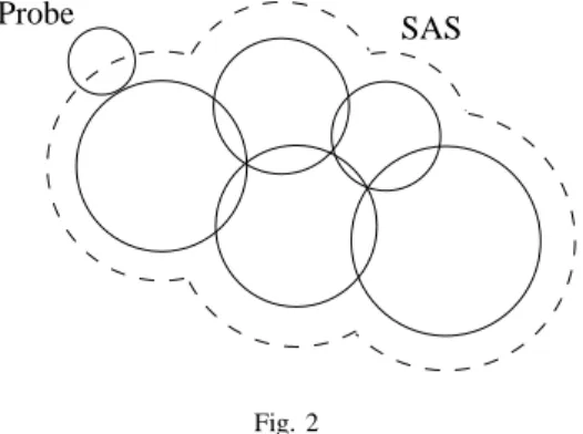
• the Solvent Accessible Surface (SAS) that is the first to
use the notion of solvent.
• the Connolly Surface (CS) that is considered as the real
surface of a molecule.
An atom can be represented as a sphere due to its Van der Waals radius. The VDWS corresponds to the sum of the spherical surface parts that are not in collision with other spheres. Figure 1 shows the Van der Waals surface of a molecule of five atoms.
VDWS
Fig. 1
VAN DERWAALS SURFACE(VDWS)OF A MOLECULE COMPOUND OF FIVE ATOMS.
The SAS, and later the CS, were defined by Lee and Richards in [13] and in [14] respectively. For the VDWS, the molecule is considered to be in the vacuum but it is a simplified model. The SAS and the CS are more realistic surfaces because they consider that the molecule is in a solvent. This solvent presence is symbolized by a probe. The SAS is drawn according to the center of this probe that rolls on the atom spheres. Generally, the probe has a radius of
1.4 ˚A (1 angstrom( ˚A)= 0.1 nanometer) in order to be able to contain a water molecule that is one of the standard solvents. Figure 2 describes the SAS of the same molecule of five atoms.
Probe SAS
Fig. 2
SOLVENT ACCESSIBLE SURFACE(SAS)OF A MOLECULE COMPOUND OF FIVE ATOMS. THE PROBE SYMBOLIZES A SOLVENT MOLECULE. IN OUR
CASE,IT IS A MOLECULE OF WATER.
For the CS, the surface is drawn according to all the points of the probe surface that touch the atom spherical surfaces. A special case occurs when a probe touches two spheres at the same time. In this case, the drawn surface corresponds to all the points of the probe surface which are oriented toward the molecule. An example of CS is shown in the figure 3 always with the same molecule of five atoms.
Probe
CS
Fig. 3
CONNOLYSURFACE(CS)OF A MOLECULE COMPOUNDED OF FIVE ATOMS. THE PROBE SYMBOLIZES A SOLVENT MOLECULE. IN OUR CASE,
IT IS A MOLECULE OF WATER.
Several methods that compute these surfaces can be found in [15], [16], [17], [18].
For our multi-objective model, we use an algorithm that computes an approximation of the SAS for a LSC. The SAS is a good compromise between quality and computational complexity. Due to the notion of solvent, it is a realistic surface and its calculus is not too expensive compared to the CS computation. The original SAS algorithm was first presented in [19], but was also recently used in [20]. It is based on look-up tables and Boolean Logic. It approximates the method of Shrake and Rupley [21].
According to this method, each atom spherical surface is represented as a set of points (figure 4). Each point is encoded
Fig. 4
REPRESENTATION OF THE SPHERICAL SURFACE OF AN ATOM WITH POINTS.
as a bit to indicate if it is in interaction with the solvent (1) or not (0). Thus surface points are represented as bit string. Due to the atom encoding, computing the area of one atom only consists of “AND” Boolean operations. Look-up tables are used to speed-up the calculus by saving Boolean masks used to approximate intersection between atom points. The SAS of a LSC allows to evaluate the penetration of the ligand into the site. In a real docking process, the ligand may try to dive into the binding site or try to modify its conformation to better suit the binding surface. In both cases, the corresponding SAS will decrease. Therefore, this criterion is essential for simulating realistic flexible docking processes.
III. METHOD
A. Multi-objective optimization problems
In a variety of applications, a problem arises that several objective functions have to be optimized concurrently. One important feature of these problems is that the different ob-jectives typically contradict each other and therefore certainly not have identical optima. Thus, the question arises how to approximate one or several particular “optimal compromises” or how to compute all optimal compromises of this multi-objective optimization problem (MOP).
A MOP can be defined as follow:
min
x∈S{F (x)}, S = {x ∈
R
n : h(x) = 0, g(x) ≤ 0},
whereF is defined as the vector of the objectives: F :R n →R k , F (x) = (f1(x), ..., fk(x)), with f1, ..., fk : R n → R, h : R n → R m, m ≤ n, and g :R n → R q. A vector v ∈ R k is said to be dominated by a vectorw ∈R k if for alli ∈ 1, ..., k w i ≤ vi andv 6= w.
A vectorv is nondominated with respect to a set P , if none
of the vectors p ∈ P dominate v. A point x ∈ S is called
optimal or Pareto optimal, if F (x) is not dominated by any
vectors F (y), y ∈ S.
B. ParadisEO platform
In order to ease the implementation of our algorithm, we have used the ParadisEO platform [22]. ParadisEO is a complete platform to design powerful optimization methods. It consists in four components:
1) ParadisEO-EO (Evolving Object) dedicated to population-based metaheuristics.
2) ParadisEO-MO (Moving Object) dedicated to single solution-based metaheuristics.
3) ParadisEO-MOEO (Multi Objective EO) dedicated to multi-objective meta-heuristics.
4) ParadisEO-PEO (Parallel EO) dedicated to parallel metaheuristics.
ParadisEO-MOEO [23] and ParadisEO-PEO have been more particularly used in our case. More information about ParadisEO is available on the official website:
(http : //paradiseo.gf orge.inria.f r).
This platform allows the user to only design the parts spe-cific to his problem in order to design effective algorithms. In our case, only solution encoding, solution evaluation and genetic operators have implemented.
C. Parallel genetic algorithms
Thanks to the ParadisEO platform, two parallel genetic algorithms have been designed: one based on the well known NSGA-II (Non-dominated Sorting Genetic Algorithm II) and the other on the IBEA (Indicator-Based Evolutionary
Algo-rithm). The first one is a standard multi-objective algorithm
used to test our model. The second one is an algorithm that has been proved better than NSGA-II on several problems. Therefore, we have test it on the docking problem.
1) Genetic Algorithms: A Genetic Algorithm (GA) works
by repeatedly modifying a population of artificial structures through the application of genetic operators (crossover and mutation) [24]. The goal is to find the best possible solution or, at least good, solutions for the problem.
2) NSGA-II and IBEA: In NSGA-II [25], the solutions
contained in the population are ranked into several classes at each generation. Individuals from the first front all belong to the first efficient set. Individuals from the second front all belong to the second best efficient set, etc. Two values are then computed for every solutions of the population. The first one corresponds to the rank the corresponding solution belongs to, and represents the quality of the solution in terms of convergence. The second one, the crowding distance, consists of estimating the density of solutions surrounding a particular point of the objective space, and represents the quality of the solution in terms of diversity. A solution is said to be better than another if it has the best rank, or in the case of a tie, if it has the best crowding distance. The selection strategy is a deterministic tournament between two random solutions. At the replacement step, only the best individuals survive, with respect to the population size. Likewise, an external population is added to the steady-state NSGA-II in order to store every potentially efficient solution found during the search.
For IBEA [26], the fitness assignment scheme is based on a pairwise comparison of solutions contained in a population by using a binary quality indicator. No diversity preservation technique is required, according to the indicator being used. The selection scheme for reproduction is a binary tournament
between randomly chosen individuals. The replacement strat-egy is an environmental one that consists of deleting, one-by-one, the worst individuals, and in updating the fitness values of the remaining solutions each time there is a deletion; this is continued until the required population size is reached. Moreover, an archive stores solutions mapping to potentially non-dominated points, in order to prevent their loss during the stochastic search process.
3) Coding: In our algorithm, the solutions are represented
according to two vectors of float corresponding to the atomic coordinates. Each atom has three coordinates (x, y and z). Figure 5 describes this coding. In our case a solution is called a “Docking Complex”. X0 Y0 Z0 X1 X2 Y1 Y2 Z1 Z2 XN−1 YN−1 ZN−1 X’0 Y’0 Z’0 X’1 Y’1 Z’1 X’2 Y’2 Z’2 X’M−1Y’M−1Z’M−1 Ligand N atoms Docking Complex M atoms Protein Fig. 5
REPRESENTATION A SOLUTION IN OUR GENETIC ALGORITHM. NANDM
ARE THE NUMBER OF ATOMS COMPOUNDING THE BINDING SITE AND THE LIGAND RESPECTIVELY.
Between two individuals, only the coordinates of the atoms change. The molecule topology is already loaded and can be used directly. The full ligand/site complex is only build during the evaluation step of an individual.
4) Operators: There are two types of operators in a
standard GA: crossover and mutation. The crossover mixes the information of two individuals, the parents, to create new individuals, the children. In our case, it swaps the ligand of two complexes. If the parent complexes are S1L1 and
S2L2, the children complexes will be S1L2 and S2L1. It
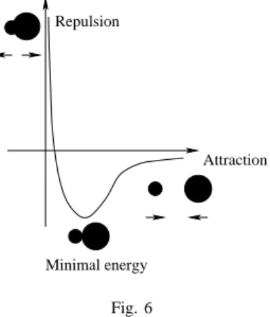
must be noticed that this type of operator can generate invalid complexes with atomic collisions. However, these complexes are penalized by the evaluation of the first objective. Its can be explained by one of the term of our first objective function: the Van der Waals term. Figure 6 details the
variation of the energy between two atoms according to the distance of their center.
Repulsion
Attraction
Minimal energy Fig. 6
VAN DERWAALS INTERACTION BETWEEN TWO ATOMS.
There is an optimal distance that minimizes the energy, but if two atoms are too close the corresponding energy become very high. That is why our first objective function will penalize such ligand/site configuration. Thus, we do not need a mechanism to repair or check the generated complexes.
Crossover operators do not add new information to the population. The parent information is just reordered in the children. Mutation adds some diversity in the new individuals just after applying the crossover. This unary operator is applied on an individual according to a global probability of mutation. Three mutation operators have been designed: rotation, translation and torsion rotation mutation. The ro-tation and translation operators provide rigid docking. The last operator adds some flexibility in the docking. If only one molecule can have its structure modified (typically the ligand) due to torsion rotation, it is a semi-flexible docking. If both molecules can be modified, it is a full flexible docking. In our case, we can make rigid, semi-flexible or full-flexible docking according to the configuration of our algorithm. The choice of mutation used depends on probabilities linked to each of them.
5) Paralleling scheme: In optimization methods, the
eval-uation step is resource consuming. Therefore, we use the well known master/slave paradigm for the individual evaluation. The master manages the GA and the slaves are used to evaluate one individual. In ParadisEO-PEO, the master is known as a runner and another process called scheduler dispatches the individuals that will be evaluated by the slaves. For instance, a parallel run with a master and ten slave needs in reality twelve processors.
IV. RESULTS
A. Test protocol
1) test data: In order to test our model, we use
lig-and/site complexes (LSC) from the CCDC/Astex data set. The original version of this data set is referenced in [27]. It corresponds to the benchmarking of the GOLD docking software. We have taken instances from the CCDC/Astex
“clean” list. It corresponds to 224 diversified instances that suit well for docking benchmarking.
Table I presents the first complexes taken from this list.
TABLE I
PROTEIN-LIGAND COMPLEXES USED FOR BENCHMARKING. PDBIS THE
PROTEINDATABANK IDENTIFIER OF THE COMPLEXES.
Protein-ligand complexes PDB
Ribonuclease A / Uridine-2’,3’-Vanadate 6rsa
HIV-1 Protease / G26 1mbi
Thymidilate / CB3 2tsc
HIV-1 Protease / G26 1htf
Glucoamylase-471 / Alpha-d-mannose 1dog
For the remaining of this article, the complexes will be designated by their corresponding Protein Data Bank identifier (PDB). The docking algorithm is the last step of a larger work-flow of molecule/molecule interaction analysis: docking@GRID. According to this work-flow, we consider that the docking algorithm starts with two proteins, a ligand and another molecule with a potential binding site, in a stable conformation gained thanks to a folding algorithm. We also consider that the protein corresponding to the ligand is already in front of the binding site.
To prepare our instances, we have used the USCF Chimera software1. The ligand has been manually extracted from its crystallographic location in order to have a seed ligand. This seed is perturbed to generate a population of diversified individuals. These perturbations combine rotation, translation and torsion rotation. All these perturbations are applied randomly a given number of times (10 by default).
Table II details the deviation between the seed ligand used to initialize the GA population and the ligand considered to be at the good location according to the crystallographic data. The computed deviation is the Root Mean Square Deviation (RMSD). According to [28], the RMSD is defined as followed: RM SD = r Pn i=1(dx 2 i + dy 2 i + dz 2 i) n (4)
In equation 4,n corresponds to the total number of atoms. dxi, dyi and dzi are the atomic coordinate differences
be-tween the ligand predicted location and its location according to the crystallographic data.
TABLE II
RMSDBETWEEN THE SEED LIGAND AND THE LIGAND IN ITS CRYSTALLOGRAPHIC LOCATION(ACCORDING TO THECCDC-ASTEX
DATA SET). THE INSTANCES ARE CITED ACCORDING TO THEIRPDB
IDENTIFIER.
Instance RMSD seed VS optimal ( ˚A)
6rsa 7.15 1mbi 7.93 2tsc 13.48 1htf 14.45 1dog 10.68 1www.cgl.ucsf.edu/chimera
2) Parameters: Our population consists in 100
individ-uals. The probabilities of crossover and mutation are 0.9 and 0.5 respectively. In our GA, the stopping criterion is a number of generations without improvement after a minimal number of generations. No improvement means no new non-dominated solution discovery. In our tests, the minimal number of generations is 1000 and the number of generations without improvement is 100.
3) Paralleling speed-up: Table III and figure 7 shows an
example of the speed-up obtained thanks the parallelization of our GA for a small population of 32 individuals using Intel Xeon 3Ghz processors. The speed-up corresponds to the ratio of the time taken with one slave and the time with more slaves (2, 4, 8, 16 and 32 respectively).
TABLE III
SPEED-UP ACCORDING TO THE NUMBER OF SLAVES. SPEED-UP CORRESPONDS TO TIME FOR1SLAVE DIVIDED BY THE TIME OFX
SLAVES.
Number of slaves Time in seconds Speed-up
1 1243.76 1 2 769.30 1.62 4 543.73 2.29 8 439.85 2.83 16 365.32 3.4 32 352.61 3.53 300 400 500 600 700 800 900 1000 1100 1200 1300 5 10 15 20 25 30 0 1 2 3 4 Time in seconds Speed-up Number of slaves 300 400 500 600 700 800 900 1000 1100 1200 1300 5 10 15 20 25 30 0 1 2 3 4 Time in seconds Speed-up Number of slaves Fig. 7
TIME(DECREASING LINE)AND SPEED-UP(INCREASING LINE)
ACCORDING TO THE NUMBER OF SLAVES USED.
According to these data, we can establish that having a number of slaves equal to the population size is not necessarily an efficient solution. It can be due to the time of communication between the master and a slave: packing an individual (master), send it (from master to slave), unpacking the individual (slave), evaluate it (slave), packing the individ-ual (slave), send it (from slave to master) and unpacking the individual for using it (master). In an individual, the ligand coordinate vector is generally very small (< 100 atoms) but
the binding site coordinate vector can be huge (more than 5000 atoms).
TABLE IV
COMPARISON OF DIFFERENT METAHEURISTICS FOR THEEpsAND THE
I−
HMETRICS BY USING AMANN-WHITNEY STATISTICAL TEST WITH A
P-VALUE OF5%. ACCORDING TO THE METRIC UNDER CONSIDERATION,
EITHER THE RESULTS OF THE ALGORITHM LOCATED AT A SPECIFIC ROW ARE SIGNIFICANTLY BETTER THAN THOSE OF THE ALGORITHM LOCATED AT A SPECIFIC COLUMN(≻),EITHER THEY ARE WORSE(≺),
OR THERE IS NO SIGNIFICANT DIFFERENCE BETWEEN BOTH(≡).
Eps I−
h
Instance algorithms IBEA NSGA II IBEA NSGA II
6rsc IBEA - ≻ - ≻
NSGA II ≺ - ≺
-1mbi NSGAIIIBEA - ≻ - ≻
≺ - ≺ -2tsc IBEA - ≡ - ≻ NSGAII ≡ - ≺ -1htf NSGAIIIBEA - ≡ - ≡ ≡ - ≡ -1dog IBEA - ≻ - ≻ NSGA II ≺ - ≺ -B. Comparison
All our tests have been run on a cluster of 64 Intel Xeon 3Ghz processors.
1) Performance Assessment: For each instance and each
metaheuristic, a set of 10 runs, with different initial
popu-lations, has been performed. In order to evaluate the quality of the non-dominated front approximations obtained for a specific test instance, we follow the protocol given in [29]. First, we compute a reference set Z⋆
N of non-dominated
points extracted from the union of all these fronts. Second, we define zmax = (zmax
1 , z2max), where zmax1 (respectively
zmax
2 ) denotes the upper bound of the first (respectively
second) objective in the whole non-dominated front approx-imations. Then, to measure the quality of an output set A
in comparison to Z⋆
N, we compute the difference between
these two sets by using the unary hypervolume metric [30],
(1.05 × zmax
1 , 1.05 × z max
2 ) being the reference point. The
hypervolume difference indicator computes the portion of the objective space that is dominated weakly byZ⋆
N and not
by A. Furthermore, we also consider the unary additive
ǫ-indicator (I1
ǫ+) that gives the minimum value by which an
approximationA has to be translated in the objective space
to dominate weakly the reference setZ⋆
N. As a consequence,
for each test instance, we obtain10 hypervolume differences
and10 epsilon measures, corresponding to the 10 runs, per
algorithm. As suggested by Knowles et al. [29], once all these values are computed, we perform a statistical analysis on pairs of optimization methods for a comparison on a specific test instance. To this end, we use the Mann-Whitney statistical test as described in [29], with a p-value lower than
10%. Note that all the performance assessment procedures
have been achieved using the performance assessment tool suite provided in PISA2 [31].
According to table IV, IBEA globally outperforms NSGA
2The package is available at http://www.tik.ee.ethz.ch/
II for the instances of our problem.
2) Docking results quality: In order to evaluate our model,
we have computed the RMSD of the ligand of our solutions with the crystallographic location of the ligand. In the literature, it is common to estimate that a docking is good for a RMSD ≤ 2.0 ˚A. Nevertheless, the standard RMSD computation is not very robust according to several factor: size of the molecule, atoms used and not used, symmetric part, etc. So it is important to analyze well each solution for estimate its quality. Furthermore, the distance between the initial solutions and the crystallographic solution is important because in most of the literature, this distance is not >10 ˚A and generally≤ 5 ˚A.
Table V summarizes the results of NSGA-II and IBEA on the five chosen instances. As the RMSD is not (and can not be) an objective of our model, all the archives generated during each run are analysed to know the quality of the encountered solutions. We have remarked that the solutions with the best RMSD are not necessary in the final archive. It can be explained by a premature convergence of our algorithm. In the same manner, one run makes on average of 225 000 evaluations. Comparing to other docking methods as Autodock (2 000 000 evaluations), it is not very high. Therefore, this number of evaluation can also significate a premature convergence of our algorithm.
TABLE V
BEST RESULTS FOR EACH INSTANCE WITH THENSGA-IIANDIBEA
ALGORITHMS. FOR EACH ALGORITHM THE BESTRMSDAND THE STANDARD DEVIATION(STD)BETWEEN THE BESTRMSDS ARE GIVEN.
NSGA-II best results IBEA best results Instance RMSD ( ˚A) std RMSD ( ˚A) std 6rsa 1.66 1.04 1.32 1.3 1mbi 5.2 0.4 4.16 0.8 2tsc 2.19 2.75 2.19 2.68 1htf 2.88 2.64 2.59 1.33 1dog 4.38 0.99 2.44 0.56
According to the RMSD of our solution and the cor-responding seed RMSD, we can estimate that our results are good for four instances (more particularly 6rsa, 2tsc and 1htf). Only 1mbi is problematic because the algorithm makes only few improvement of the RMSD (according to the RMSD of the seed). An analysis of the 1mbi instance shows that the ligand is a very tiny molecule (9 atoms) that has to be put in a big binding site (see Figure 8). Therefore, there are a lot of potential binding mode for the ligand, maybe of equivalent quality.
According to the algorithm comparison, IBEA gives better or equivalent results on each instances. We can notice that the standard deviations are better for NSGA-II on 6rsa and 1mbi instances. This can be explained by the size of the instances because 6rsa and 1mbi are the smallest instances of our dataset.
IBEA has been already proved better than NSGA-II for several problems. Our results confirm this remark.
In order to compare visually a result of docking, the figure 9 shows the crystallographic complex of the 6rsa
Fig. 8
LIGAND/SITE COMPLEX COMING FROM CRYSTALLOGRAPHIC DATA FOR THE1MBI INSTANCE.
instance. Figure 10 and figure 11 represent the complex with the minimal RMSD gained with the NSGA-II and IBEA algorithms respectively.
Fig. 9
LIGAND/SITE COMPLEX COMING FROM CRYSTALLOGRAPHIC DATA FOR THE6RSA INSTANCE.
NSGA-II proposes a ligand that is partially centered in the binding site. The ligand has not find its right conformation in the binding site.
The IBEA solution has a lower RMSD because the ligand is better centered into the binding site.
Complementary tests are currently made in order to extend the number of instances tested and compare our approach with other works of the literature. Nevertheless, according to our tests, our model has been validated and gives promising results.
V. CONCLUSIONS
In this article, a new bi-objective model for the molecular docking problem has been proposed. This model has been validated thanks to instances of high confidence dedicated to docking benchmarking. Our model can be easily used with other energy function (and force field) and/or other molecular
Fig. 10
LIGAND/SITE COMPLEX COMING FROM THE INDIVIDUAL HAVING THE
BESTRMSD (1.66)WITH THENSGA-IIALGORITHM.
Fig. 11
LIGAND/SITE COMPLEX COMING FROM THE INDIVIDUAL HAVING THE
BESTRMSD (1.32)WITH THEIBEAALGORITHM.
surfaces. A tri-objective version of our model is being tested. The third objective is a robustness objective. It describes the quality of the ligand/site complex by making a sampling of the energetic landscape around a current individual. However, this model is very time and resource consuming and has to be improved in order to be used efficiently (grid com-puting). Furthermore, in order to improve the diversity of our population of solutions to prevent a potential premature convergence, new operators are planned to be added as the reverse mutation. The reverse mutation consists in making a big rotation of 180 of the ligand in order to increase the speed of convergence. This type of mutation can be useful in the case of a ligand well entered into the binding site but in the bad side so the associated RMSD is not low. In this case, it cannot be reversed by small rotations due to the lack of space. With the improvement of the algorithm behaviour, we are getting a powerful docking method that will be available on-line throw the Docking@GRID platform (http://docking.futurs.inria.fr).
REFERENCES
[1] D. Goodsell and A. Olson, “Automated docking of substrates to proteins by simulated annealing,” Proteins: Structure, Function and Genetics, vol. 8, pp. 195–202, 1990.
[2] G. Jones, P. Willet, and R. Glen, “Molecular recognition of receptor sites using a genetic algorithm with a description of desolvation,” Journal of Molecular Biology, vol. 245, no. 1, pp. 43–53, 1995. [3] J.-M. Yang, “An Evolutionnary Approach for Molecular Docking,” in
GECCO’03. LNCS 2724, 2003, pp. 2372–2383.
[4] G. Morris, D. Goodsell, R. Halliday, R. Huey, W. Har, R. Belew, and A. Olson, “Automated docking using a lamarckian genetic algorithm and an empirical binding free energy function,” Journal of Computa-tional Chemistry, vol. 19, pp. 1639–1662, 1998.
[5] S. Janson, D. Merkle, and M. Middendorf, “Molecular docking with a multi-objective Particle Swarm Optimization,” Applied Soft Comput-ing, 2007, doi:10.1016/j.asoc.2007.05.005.
[6] O. Kord, T. St¨utzle, and T. Exner, “An Ant colony optimization ap-proach to flexible protein-ligand docking,” Swarm Intelligence, 2007, doi: 10.1007/s11721-007-0006-9.
[7] T. Ewing and I. Kuntz, “Critical evaluation of search algorithms for automated molecular docking and database screening,” Journal of Computational Chemistry, vol. 18, no. 9, pp. 1175–1189, 1997. [8] M. Rarey, B. Kramer, T. Lengauer, and G. Klebe, “A fast flexible
docking method using an incremental construction algorithm,” Journal of Molecular Biology, vol. 261, no. 3, pp. 470–489, 1996.
[9] B. Bursulaya, M. Totrov, R. Abagyan, and C. Brooks, “Comparative study of several algorithms for flexible ligand docking,” Journal of Computer-Aided Molecular Design, vol. 17, no. 11, pp. 755–763, november 2003. [Online]. Available: http://abagyan.scripps.edu/ [10] A. Oduguwa, A. Tiwari, S. Fiorentino, and R. Roy, “Multi-Objectice
Optimisation of the Protein-Ligand Docking Problem in Drug Discov-ery,” in GECCO’06, July 8-12 2006, seattle, Washington, USA. [11] M. Yamagishi, N. Martins, G. Neshich, W. Cai, X. Shao, A. Beautrait,
and B. Maigret, “A fast surface-matching procedure for protein-ligand docking,” Journal of Molecular Modeling, vol. 12, pp. 965–972, 2006. [12] A.-A. Tantar, N. Melab, E.-G. Talbi, and B. Toursel, “A Parallel Hybrid Genetic Algorithm for Protein Structure Prediction on the Computational Grid,” Elsevier Science, Future Generation Computer Systems, vol. 23, no. 3, pp. 398–409, 2007.
[13] B. Lee and F. Richard, “The interpretation of protein structures: Estimation of static accessibility,” Journal of Molecular Biology, vol. 55, pp. 379–400, 1971.
[14] F. Richard, “Areas, volumes, packing and protein structure,” Annual Review of Biophysics and Bioengineering, vol. 6, pp. 151–176, 1977. [15] R. Fraczkiewicz and W. Braun, “Exact and Efficient Analytical Cal-culation of the Accessible Surface Areas and Their Gradients for Macromolecules,” Journal of Computational Chemistry, vol. 19, no. 3, pp. 319–333, 1998.
[16] N. Futamura, S. Aluru, D. Ranjan, and K. Mehrotra, “Efficient Algo-rithms for Protein Solvent Accessible Surface Area,” In Proceedings of the The Fourth International Conference on High-Performance Computing in the Asia-Pacific Region, vol. 2, pp. 586–592, 2000, iSBN: 0-7695-0589-2.
[17] J. Ryu, R. Park, and D. Kim, “Connoly Surface on an Atomic Structure via Voronoi Diagram of Atoms,” Journal of Computer Science and Technology, vol. 21, no. 2, pp. 255–260, 2006.
[18] Y. Vorobjev and J. Hermans, “SIMS: Computation of a Smooth Invariant Molecular Surface,” Biophysical Journal, vol. 73, pp. 722– 732, 1997.
[19] S. L. Grand and J. K.M. Merz, “Rapid Approximation to Molecular Surface Area via the Use of Boolean Logic and Look-up Tables,” Journal of Computational Chemistry, vol. 14, pp. 349–352, 1993. [20] A. Leaver-Fay, G. Butterfoss, J. Snoeyink, and B. Kuhlman,
“Main-taining solvent accessible surface area under rotamer substitution for protein design,” Journal of Computational Chemistry, vol. 28, no. 8, pp. 1336–1341, 2007.
[21] A. Shrake and J. Rupley, “Environment and exposure to solvent of protein atoms. lysozyme and insulin,” Journal of Molecular Biology, vol. 79, no. 2, pp. 351–364, 1973.
[22] S. Cahon, N. Melab, and E.-G. Talbi, “ParadisEO: A Framework for the Reusable Design of Parallel and Distributed Metaheuristics,” Journal of Heuristics, vol. 10, no. 3, pp. 357–380, 2004.
[23] A. Liefooghe, M. Basseur, L. Jourdan, and E.-G. Talbi, “ParadisEO-MOEO: A Framework for Multi-Objective Optimization,” in Proceed-ings of EMO’2007, Springer-Verlag, Ed., 2007, pp. 457–471.
[24] J. Holland, Adaptation in Natural and Artificial Systems. University
of Michigan Press, 1975.
[25] K. Deb, A. Pratap, S. Agarwal, and T. Meyarivan, “A fast and elitist multi-objective genetic algorithm: NSGA-II,” IEEE Transaction on Evolutionary Computation, vol. 6, no. 2, pp. 181–197, 2002. [26] S. E. Zitzler, “Indicator-based selection in multiobjective search,”
Parallel Problem Solving from Nature, PPSN VIII, vol. 3242, pp. 832– 842, 2004.
[27] M. Hartshorn, M. Verdonk, G. Chessari, S. Brewerton, W. Mooij, P. Mortenson, and C. W. Murray, “Diverse, High-Quality Test Set for the Validation of Protein-Ligand Docking Performance,” Journal of Medical Chemistry, vol. 50, pp. 726–741, 2007.
[28] R. Thomsen, Computational Intelligence in Bioinformatics. Institute
of Electrical and Electronis Engineers, Inc., 2008, ch. 8.
[29] J. Knowles, L. Thiele, and E. Zitzler, “A tutorial on the performance assessment of stochastic multiobjective optimizers,” Computer Engi-neering and Networks Laboratory (TIK), ETH Zurich, Switzerland, Tech. Rep., 2006, (revised version).
[30] E. Zitzler and L. Thiele, “Multiobjective evolutionary algorithms: A comparative case study and the strength pareto approach,” IEEE Transactions on Evolutionary Computation, vol. 3, no. 4, pp. 257– 271, 1999.
[31] S. Bleuler, M. Laumanns, L. Thiele, and E. Zitzler, “PISA — a platform and programming language independent interface for search
algorithms,” in EMO’2003, ser. LNCS, vol. 2632. Faro, Portugal: