Connecting Symbols to Primitive Percepts using
Expectation as Feedback
by
Manushaqe Muco
S.B., Massachusetts Institute of Technology (2015)
M.Eng., Massachusetts Institute of Technology (2017)
Submitted to the Program in Media Arts and Sciences,
School of Architecture and Planning,
in partial fulfillment of the requirements for the degree of
Master of Science in Media Arts and Sciences
at the
MASSACHUSETTS INSTITUTE OF TECHNOLOGY
September 2020
c
○ Massachusetts Institute of Technology 2020. All rights reserved.
Author . . . .
Program in Media Arts and Sciences
August 07, 2020
Certified by . . . .
Gerald Jay Sussman
Panasonic Professor of Electrical Engineering
Thesis Supervisor
Accepted by . . . .
Tod Machover
Academic Head, Program in Media Arts and Sciences
Connecting Symbols to Primitive Percepts using Expectation
as Feedback
by
Manushaqe Muco
Submitted to the Program in Media Arts and Sciences, School of Architecture and Planning,
on August 07, 2020, in partial fulfillment of the requirements for the degree of
Master of Science in Media Arts and Sciences
Abstract
This thesis is a step towards understanding and building mechanisms that connect symbols to primitive percepts. Symbols, such as those used in symbolic reasoning and language, are more intuitive to us humans since our languages and artifacts are highly symbolic. On the other hand, primitive percepts are results of processes that combine large amounts of evidence numerically, and are thus opaque to our human understanding.
Inspired by an optical illusion known as Kanizsa’s Triangle, I propose that expec-tation is essential to perception at every layer, including the very lowest levels. My proposal is that expectations generate hallucinations, that when mutually constrained with the sense data, produce a reasonable interpretation of that data. Furthermore, the mechanisms that project expectations may just be what connects, at an appro-priate level, symbols to percepts.
To engineer such mechanisms in an artificial machine, I start with feedback at every layer as a simple mechanism for projecting expectations. I then present a multi-layered distributed structure that incorporates such feedback expectations, and that recognizes and hallucinates images of digits using a bidirectional mutual constraining process. In this process the higher layers work as critics on lower layers, filling in details and removing noise to improve the data at that level.
Thesis Supervisor: Gerald Jay Sussman
Connecting Symbols to Primitive Percepts using Expectation
as Feedback
by
Manushaqe Muco
This thesis has been reviewed and approved by the following committee members:
Advisor . . . .
Gerald Jay Sussman
Panasonic Professor of Electrical Engineering
MIT Department of Electrical Engineering and Computer Science
Thesis Reader . . . .
Joseph A. Paradiso
Alexander W Dreyfoos (1954) Professor
MIT Program in Media Arts and Sciences
Thesis Reader . . . .
Howard Shrobe
Principal Research Scientist
MIT Computer Science & Artificial Intelligence Lab
Acknowledgments
To Howard Shrobe and Joseph Paradiso for giving this outside-of-the-box idea a chance.
To the students at Personal Robots, and those at Media Lab at large. Particu-larly Ravi Tejwani, my good friend, and Pat Pataranutaporn; both people I could have interesting conversations with.
To Marta Kiljan, who is like a sister to me, and who always makes sure the dia-grams in my projects look up to par.
To Raudel Hernandez, one of my best friends, who has been my lifeline in and out of MIT.
Last but not least, to Gerry Sussman, for being a friend, a mentor, and someone I look up to. For always believing in me, and for encouraging extraordinary ideas and perseverance.
Contents
1 Introduction 15
1.1 Expectation as Essential to Perception . . . 16
1.2 Engineering Mechanisms for Expectation . . . 18
1.3 Organization of Thesis . . . 18 2 Architecture 20 2.1 Data Set . . . 21 2.2 A Bigger Picture . . . 21 2.3 Architecture Model . . . 23 2.3.1 Modules . . . 23
2.3.2 Patterns, Filters, and Expectations . . . 24
2.3.3 Numerical and Waltz Layers . . . 27
2.4 Distinctiveness from Current Approaches . . . 30
3 Algorithm 33 3.1 Components . . . 33
3.2 The Module Settles . . . 35
3.3 Communicating Between Modules . . . 38
3.4 The Architecture Settles . . . 39
4 Experimental Results 42 4.1 Noise . . . 42
4.3 Recognition and Interpretation of Patterns . . . 44
5 Contributions 52
5.1 Adversarial attacks . . . 53 5.2 Future Work . . . 55
List of Figures
1-1 One variation of Kanizsa’s Triangle where a certain configuration of Pac-Man-shaped black circles evokes the perception of a white triangle, seemingly brighter in luminance than the background. If we shift the orientation of the Pac-Man circles as shown in the image to the right, a triangular shape is no longer perceived. . . 17 1-2 A second variation of Kanizsa’s Triangle where the evoked bright
tri-angle in the middle seems to occlude the three black Pac-Man-shaped circles and a black-outlined triangle. . . 17 2-1 Image appearing on page 189 of Waltz’s PhD thesis document,
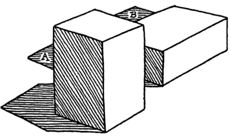
incor-porating shadows and an object obscuring another. His work handles many more such examples, including cracks, more blocks, and more complex positional relations between blocks. . . 22 2-2 The architecture is composed of indexed modules, where each module
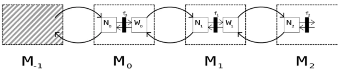
consists of a numerical layer and a waltz layer, communicating with each other through feedback connections for mutual constraining. A filter layer in between facilitates the application of convolutional filters, as well as helps impose projected expectations. Once a module has settled, it can send information to other modules using similar feedback connections, but this time in between modules. Module 𝑀−1 is special
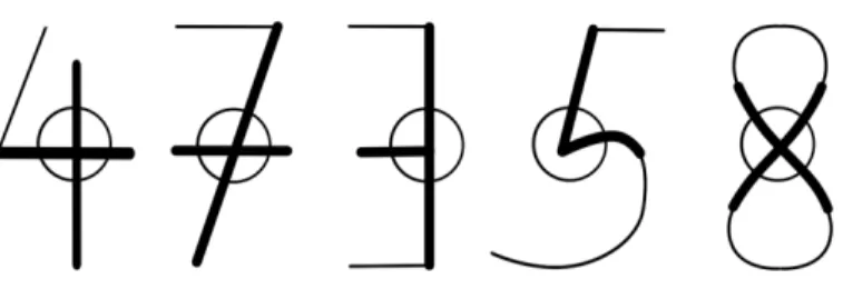
2-3 Visualizing expectations for digit parts in higher level modules: the straight crossover in number 4, the titled crossover in number 7, the t-junction in number 3, the cusp in number 5, and the X-crossover in number 8. . . 26 2-4 Schematic diagram illustrating the interconnections between the
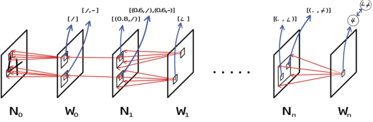
nu-merical and waltz layers in finer details. While at first glance it seems like a typical feedforward processing of a digit, note that the red connec-tions between the layers are bidirectional arrows, denoting the ability to propagate information in two directions, for mutual constraining. The number of layers (and as a consequence the number of modules as well) depends on the size of filters we experiment with at every level. 28 3-1 Visualization of how the amount of computation done inside the
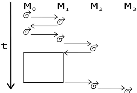
ar-chitecture grows diagonally, as spanned by time and the number of modules. The white box indicates a repeating block of computation until both modules 𝑀0 and 𝑀1 have happily settled. . . 40
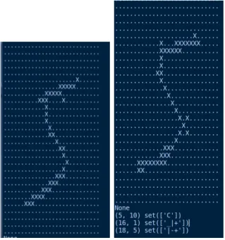
4-1 The architecture recognizes a cusp in cell (5, 10) of 𝑊2, and a big corner
in cell (16,1), but a filter size of 5x5 or 7x7 can’t link the two in layers 𝑁3 and 𝑊3. Also note that the way the digit is printed in the console
only accounts for non-background pixels. Only when converting to a grayscale image, such as the ones you see in the noise and hallucination examples, can you see the differences in pixel strength. . . 46 4-2 The result of executing the command "print w2" in the console, offering
a glimpse at how the layer’s representation looks like. The string "C" is the symbolic representation chosen for the cusp pattern. . . 47
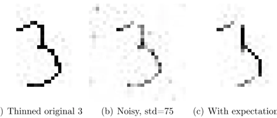
4-3 STD=75. The original image is a digit 3, at index 30000 in the MNIST training set. The architecture has removed spurious dots in the back-ground and also changed the shape of the number to straighter lines. This is expected, because the architecture’s lower level expectations are straight lines, and higher level expectations build on combinations of these straight lines as a result. . . 49 4-4 The same digit as above, at index 30000 in the MNIST training set,
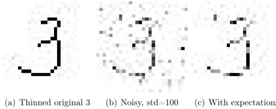
run under a noise with STD=100. The architecture fills in contour lines as predicted, but the bottom curve of the number 3 is too broken apart for the digit to be perceived as a single unit by the architecture. 49 4-5 Continuing with the same digit, at index 30000 in the MNIST
train-ing set, run under a noise with STD=120. The image is distorted beyond human recognition, and having cleared the background noise, the architecture only perceives a collection of lines. . . 49 4-6 STD=100 applied to a badly-written digit 3, at index 675 of the MNIST
training data. We start seeing an example of patterned noise, where the architecture perceives evidence for a small line next to the digit it has cleaned up. . . 50 4-7 STD=120. The original image is a digit 0, at index 57634 in the MNIST
training set. The noise has deformed the image to something that looks more like a C, and therefore the architecture doesn’t fully complete the image to a 0 after running. At first glance it may seem like the architecture has not removed all the noise, although it has removed it for the largest part. However, it is more like the "noise" that remained ended up being recognized as contributing to patterns of lines, because the filter lines are only 5 pixels long. It seems as if the architecture perceives the image as a C-shape and other small separate lines. . . . 50
4-8 STD=140. I decided to run the same image as above at a standard deviation where even for humans it becomes hard to distinguish the digit. Most of the noise is removed, except patterned noise. And the original digit lines that can still be recognized by the architecture are filled in. . . 51 4-9 Because of its expectation mechanisms of straight lines and
combina-tions of straight lines, the architecture hallucinates a more polygonal digit 0 in its retina, and causes the presented input to also transform as a result. . . 51 4-10 The architecture changes a badly-written 8 digit into an hallucinated
input that more closely resembles digit 1. . . 51 5-1 In this simple linear model, the points on the right of the dividing
hyper-plane are considered as Xs, while points on the left are regarded as Os. The red X in the upper-right corner is a point that the model "believes" to exist because of the nature of its own modeling. However, this is not a point that has been witnessed by the inputs the model has come across. . . 54
Chapter 1
Introduction
The question of how symbols arise from perceptual processes remains the holy grail of artificial intelligence.
One approach has been to build systems from the bottom up, by grounding them in sensory information from the physical world, such as visual information. The processes of such systems usually combine large amounts of evidence numerically, and we still don’t have good ways of assigning symbols to the results of those processes. For example, the internals of the most successful of these systems—convolutional neural networks, provide only sets of numerical weights and node activation values without any significant symbolic interpretation.
Although the underlying mechanisms may differ, perceptual systems in humans are opaque for similar reasons. We may be able to explain that we moved out of the road because we heard the loud sound of what we presumed to be an oncoming car, but we cannot quite give a symbolic justification of the perception of a (loud) sound. Both biological and artificial perception depends on mechanisms that are primitive, and there is little commonality between low-level languages, such as the frequency of a neuron firing or the weight of a connection, and high-level languages, such as highly symbolic ones like (human) natural language.
As we descend the levels of complexity, we end up reaching primitive percepts, such as smells or sounds, that cannot be further broken down into meaningful parts. However, by connecting these primitive percepts to symbols we can combine them
into compound structures that become coherent stories, such as the ones we humans tell to explain our behavior: “I heard a loud sound and turned my head. I saw a quickly oncoming car and moved out of the way.”
The immediate question then becomes: how do we build mechanisms for connect-ing symbols to primitive percepts, if these mechanisms seem to be opaque to our human interpretation?
1.1
Expectation as Essential to Perception
Perhaps we can gain cues from the way our visual system sees the world, especially when things turn strange.
Optical illusions are well-documented cases of images and phenomena, that trick our visual system into perceiving things differently from what they really are. For example, the familiar rabbit-duck illusion is an instance of an ambiguous figure in which either a rabbit or a duck can be seen, but never at the same time. If we regard optical illusions as a byproduct of mechanisms optimized for various tasks—including visual, we can begin to think about what these byproduct observations tell us about the mechanisms at play.
I was inspired by an illusory contour illusion known as Kanizsa’s Triangle, where the right configuration of Pac-Man-shaped black circles causes the human visual sys-tem to hallucinate the presence of a bright white triangle in the middle. Typically the triangle seems brighter than the background even though the luminance is homo-geneous in reality. Prompted by this example, I propose the notion of expectation as essential to perception at every layer, including the very lowest levels.
The idea is that the expectations generate hallucinations that, when mutually constrained with the sense data, produce a reasonable interpretation of that data. The mechanisms that project expectations are important because they may just be what connects, at an appropriate level, symbols to percepts.
Returning to the example of Kanizsa’s Triangle, the combined cues from the con-figuration of black circle cut-out corners and their appropriate physical proximity
propagates upwards in our visual system, possibly activating the expectation of an edge. This expectation, along with others related to luminance and edge combina-tions, is projected downwards, filling in the details in the lower layers, and eventually causing us to see a bright white triangle that isn’t really there. In other words, partial information from separate image fragments in a certain orientation and proximity is enough for our visual system to hallucinate an actual triangle.
Figure 1-1: One variation of Kanizsa’s Triangle where a certain configuration of Pac-Man-shaped black circles evokes the perception of a white triangle, seemingly brighter in luminance than the background. If we shift the orientation of the Pac-Man circles as shown in the image to the right, a triangular shape is no longer perceived.
Figure 1-2: A second variation of Kanizsa’s Triangle where the evoked bright triangle in the middle seems to occlude the three black Pac-Man-shaped circles and a black-outlined triangle.
failure, but rather as a way to enhance the robustness of a perceptual system is similar in spirit to what Sussman and Beal[1] have also proposed in a paper presented to the 2008 AAAI Fall Symposium, on naturally-inspired artificial intelligence.
1.2
Engineering Mechanisms for Expectation
I propose feedback at every layer as a simple mechanism for projecting expectations; that is, a simple mechanism by which symbols can affect and be affected by perception. I then design a multi-layered distributed structure that incorporates this notion of feedback expectations, and that recognizes and hallucinates images using a bidi-rectional mutual constraining process, where higher layers work as critics1 on lower
layers, filling in details and removing noise to improve the data at that level. I present this architecture as an existence proof on the power of expectation mechanisms and a tool for thinking about how such mechanisms can aid us in building machines that we can understand and learn from.
Although this dissertation focuses on symbolic correlates to visual primitive per-cepts, which I study by experimenting on low-level visual data, the resultant feedback expectation mechanisms are applicable to any level and type of perception or combi-nation of thereof; offering an explacombi-nation of strange perceptual phenomena in humans and more importantly, providing a path in bridging the discreteness of symbols with the statistical nature of the evidence presented by the real world. When it comes to immediate engineering concerns, as machines and algorithms become prevalent in our lives and make decisions for us, expectation mechanisms could also be used to provide explanation, and to ameliorate the problem of adversarial attacks.
1.3
Organization of Thesis
Chapter 2: Architecture. Specification of the architecture and the problem do-main in which it operates, including its distinctive features from current prevailing
ideas and methods.
Chapter 3: Algorithm. Conceptual description of how the feedback expectation mechanism operates, as well as its algorithmic implementation.
Chapter 4: Experimental Results. Experimental results providing details on the architecture’s performance, including a detailed analysis and discussion of the results presented.
Chapter 5: Contributions. Concisely reiterating the main contributions of the thesis, as well as providing a vision of next steps and the place of this work in the bigger picture of how symbols connect to the statistical evidence of our senses. Appendix A: Python Code.
Chapter 2
Architecture
In this chapter I specify the system’s architecture, along with the motivation for choosing to structure the problem as I have.
Briefly, the architecture consists of a succession of modules, where each module consists of two layers of cells, a waltz1 layer, and a numerical layer. Each waltz
cell stores a partial information set of symbolic expectations for a given size of its receptive field over the layer below. Each numerical cell is a numerical-symbolic hybrid containing a confidence value for each pattern computed in earlier layers, that caused the current cell to be activated. Note that a computational pattern can also become an explicit expectation: we can have a numerical cell with high confidence that its current activation results from the computation of a corner, as well as corner expectations in the appropriate waltz layers.
Each module is also conceptualized with a filter layer in between the numerical and waltz layer, to facilitate the convolutional application of the module’s filters (computational patterns) when the information is flowing upwards, from lower layers to higher layers, and help impose expectation patterns when the information flows downwards, from higher layers to lower layers.
The architecture is judged to be successful with regards to two aspects. The
1Named after David Waltz, in honor of his 1972 PhD thesis on generating semantic descriptions
from drawings of scenes with shadows[16]. His salient idea of partial information structures that can be merged by intersection is something that inspired the structure and workings of these layers in my architecture.
first is the ability to clean up and improve the original image presented to it as an input, thus displaying the ability to fill in details (or hallucinate) and remove noise. The second aspect is the ability to recognize, in its inner layers, patterns and combinations of patterns, from lines to corners, crossings, and t-junctions. Ultimately, as more layers are added, some waltz layer will have cells with a receptive field big enough to cover the entire input image. The activation of any such waltz cell can be recognized as resulting from a combination and mutual constraints of more primitive image components to make a coherent interpretation of the image.
2.1
Data Set
The system operates on the widely-used MNIST[10] dataset, a database of handwrit-ten digits, grayscaled and size-normalized to fit a 28x28 pixel bounding box. Each pixel is an unsigned char of 1 byte, and takes values from 0 to 255 (white background). Each digit is thus written in shades of dark over a white background.
While the ability to operate on natural images is important for systems to be deployed in the real world, digits provide a good starting point for studying and designing a nascent architecture. This because we already know what the answer should be: we can come up with plausible and limited guesses as to what the projected expectations for digits could look like on a symbolic level. For example, the slanted bottom curve of the number 9 could be a possible expectation for one of the system’s layers to have. We especially should not like an architecture to work in the context of something that we do not understand.
2.2
A Bigger Picture
If optical illusions inspired my notion of expectations, the inspiration for the workings of the waltz cells came from David Waltz’s 1972 PhD work, "Generating Semantic Description from Drawings of Scenes with Shadows"[16]. In his work, an object was interpreted as a set of physically realizable semantic labels associated with it, and such
a set was found through satisfying constraints with regards to neighboring objects and the background.
As shown in figure 2-1, the drawings from Waltz’s dissertation are too ambitious for the scope of this work, both in resolution size and the complexity of object rela-tionships. However, I am presenting my own architecture as a structure that needs to already be in place to allow for building systems that can interpret object scenes. In fact, this same architecture can be generalized and extended towards such a system, because it already incorporates all the necessary building blocks.
For example, just as the context of surrounding objects can be used to constrain all the possible interpretations, waltz cells already make use of the adjacency of digit parts to rule out impossibilities, working as critics when sending feedback to the cor-responding numerical layer below. The next step would be to recreate something like Waltz’s highly-symbolic program for interpreting objects, in a distributed, grounded in real data architecture, that also uses expectations.
Figure 2-1: Image appearing on page 189 of Waltz’s PhD thesis document, incor-porating shadows and an object obscuring another. His work handles many more such examples, including cracks, more blocks, and more complex positional relations between blocks.
2.3
Architecture Model
I give a high-level description of the system’s structure and its workings by following the computational flow after an image is presented to its "retina".
2.3.1
Modules
As shown in figure 2-2, the architecture consists of a succession of indexed modules, where each module is composed of a numerical layer and a waltz layer. Within the module, the numerical and waltz layers communicate with each other through feed-back connections for mutual constraining. A filter layer in between the two facilitates the application of convolutional filters, and also helps impose projected expectations. When the module receives new information, either from higher levels through its waltz layer or from lower levels through its numerical layer, it is jolted out of its equi-librium state. Constraint computations flow back and forth between the numerical and waltz layers, until the module eventually settles. Only when the module has set-tled, can it send information to other modules, to which it is connected using similar feedback connections.
Starting from index zero, each module has its own collection of expectations and filters, and the filter size determines the size of the receptive field for the module’s waltz cells. For example, a 3x3 filter size allows for a waltz cell to be connected to and oversee 9 numerical cells in the layer below.
For the rest of this document I use retina to denote the input digit projection onto numerical layer 𝑁0, because that is where the interesting computation begins to
happen. However, the actual MNIST digit is first presented to what I dub as mod-ule 𝑀−1, a special module that consists only of thinning expectations. Because the
filters and expectations of module 𝑀0 are idealized versions of lines with thickness of
one pixel, module 𝑀−1 projects expectations to thin the presented digit to
approxi-mately that desired thickness. The thinning process is achieved using the Zhang-Suen thinning algorithm[20] with thresholding[5].
Figure 2-2: The architecture is composed of indexed modules, where each module consists of a numerical layer and a waltz layer, communicating with each other through feedback connections for mutual constraining. A filter layer in between facilitates the application of convolutional filters, as well as helps impose projected expectations. Once a module has settled, it can send information to other modules using similar feedback connections, but this time in between modules. Module 𝑀−1 is special in
that it only contains thinning expectations.
2.3.2
Patterns, Filters, and Expectations
The filters in my architecture are used in the familiar way convolutional filters are used in conventional practice: as pattern-matching templates scanned across the ac-tivations of the cells of a given layer. However, the coefficients of the filters are discretized to 0s and 1s. The mathematical operation of a filter with the region it is convolved with is element-wise multiplication followed by summation. This approxi-mately implements an AND operation of activations or smaller patterns.
The simplest filters belong to module 𝑀0, and they are lines of four different
orientations: vertical, horizontal, and two possible diagonals. A 3x3 case of such filters is shown below:
⎡ ⎢ ⎢ ⎢ ⎣ 0.0 1.0 0.0 0.0 1.0 0.0 0.0 1.0 0.0 ⎤ ⎥ ⎥ ⎥ ⎦ ⎡ ⎢ ⎢ ⎢ ⎣ 0.0 0.0 0.0 1.0 1.0 1.0 0.0 0.0 0.0 ⎤ ⎥ ⎥ ⎥ ⎦ ⎡ ⎢ ⎢ ⎢ ⎣ 1.0 0.0 0.0 0.0 1.0 0.0 0.0 0.0 1.0 ⎤ ⎥ ⎥ ⎥ ⎦ ⎡ ⎢ ⎢ ⎢ ⎣ 0.0 0.0 1.0 0.0 1.0 0.0 1.0 0.0 0.0 ⎤ ⎥ ⎥ ⎥ ⎦
Once the system can recognize simple line patterns, these patterns can be com-bined into more complex ones. For example, the filters in module 𝑀1 are weighted
corners, and acute corners. ⎡ ⎢ ⎢ ⎢ ⎣ (0.0, ?) (1.0, 𝑣𝑒𝑟𝑡𝑖𝑐𝑎𝑙) (0.0, ?) (0.0, ?) (1.0, 𝑣𝑒𝑟𝑡𝑖𝑐𝑎𝑙) (0.0, ?) (0.0, ?) (1.0, 𝑣𝑒𝑟𝑡𝑖𝑐𝑎𝑙) (0.0, ?) ⎤ ⎥ ⎥ ⎥ ⎦ ⎡ ⎢ ⎢ ⎢ ⎣ (0.0, 𝑢𝑛𝑘𝑛𝑜𝑤𝑛) (1.0, ℎ𝑜𝑟𝑖𝑧𝑜𝑛𝑡𝑎𝑙) (1.0, ℎ𝑜𝑟𝑖𝑧𝑜𝑛𝑡𝑎𝑙) (1.0, 𝑣𝑒𝑟𝑡𝑖𝑐𝑎𝑙) (0.0, ?) (0.0, ?) (1.0, 𝑣𝑒𝑟𝑡𝑖𝑐𝑎𝑙) (0.0, ?) (0.0, ?) ⎤ ⎥ ⎥ ⎥ ⎦ ⎡ ⎢ ⎢ ⎢ ⎣ (1.0, ℎ𝑜𝑟𝑖𝑧𝑜𝑛𝑡𝑎𝑙) (1.0, ℎ𝑜𝑟𝑖𝑧𝑜𝑛𝑡𝑎𝑙) (0.0, 𝑢𝑛𝑘𝑛𝑜𝑤𝑛)] (0.0, ?) (1.0, 𝑑𝑖𝑎𝑔𝑜𝑛𝑎𝑙1) (0.0, ?) (1.0, 𝑑𝑖𝑎𝑔𝑜𝑛𝑎𝑙1) (0.0, ?) (0.0, ?) ⎤ ⎥ ⎥ ⎥ ⎦
In the 3x3 case above, a long vertical line filter is a combination of smaller vertical lines in the appropriate positions, one possible straight corner is the combination of horizontal and vertical smaller lines, and the acute corner of horizontal and diagonal ones. The ? symbol means we don’t care about the pattern in that position because it will be multiplied by zero during the convolution. The unknown symbol on the other hand, will become important once we get to deploying expectations.
Expectations are made explicit in the system, and when it comes to the coding of their patterns, expectations and filters reuse the same patterns. That is, for each filter pattern there’s also an expectation of that pattern: there are line expectations, and corner expectations, and so on. The difference comes from how the patterns are applied.
A filter pattern is applied over the activation of numerical cells in the receptive field of a waltz cell, and if the pattern matches to some great extent, the waltz cell sees the pattern of that filter. For example, a waltz cell in layer 𝑊0 may see a vertical
line in that region of the retina. When the same pattern is imposed as an expectation from a waltz cell over its receptive field, it will suppress the activation of numerical cells in the positions with 0 coefficients and excite the numerical cells in the positions with 1 coefficients. In more complex patterns, the positions denoted by ? will also
be suppressed.
Returning to the unknown notation in the straight corner pattern, the expectations for that corner in waltz layer 𝑊1 will neither suppress nor excite the corresponding
numerical cell in 𝑁1. The reason is that module 𝑀1 does not have the appropriate
context to decide what to do with that region. Module 𝑀2however does have a bigger
context, and its expectations may convey to module 𝑀1 that the unknown area must
be filled with a horizontal or vertical line to complete the corner. Here, context refers to the size of the retina the waltz cells of each module see. Because we are convolving at each level, each successive waltz cell sees a larger and larger portion of the original retinal display, and the result is shift-invariant.
Depending on the size we choose for the filters at each module, modules 𝑀2 and
𝑀3 will have more complex expectations and filters, such as the crossovers found in
the digits 4 and 7, the t-junction in number 3, etc. Figure 2-3 shows a visualization of such expectations and filters, followed by a 3x3 coding of the 7 crossover and the 3 t-junction as filter patterns.
Figure 2-3: Visualizing expectations for digit parts in higher level modules: the straight crossover in number 4, the titled crossover in number 7, the t-junction in number 3, the cusp in number 5, and the X-crossover in number 8.
A 7 crossover pattern is the weighted combination of long horizontal and long diagonal lines, and the 3-junction makes use of long horizontal and long vertical lines. Other patterns for filters and expectations can be found in Appendix A.
⎡ ⎢ ⎢ ⎢ ⎣ (0.0, ?) (0.0, ?) (1.0, 𝑙𝑜𝑛𝑔𝑑𝑖𝑎𝑔𝑜𝑛𝑎𝑙1) (1.0, 𝑙𝑜𝑛𝑔ℎ𝑜𝑟𝑖𝑧𝑜𝑛𝑡𝑎𝑙) (0.0, 𝑢𝑛𝑘𝑛𝑜𝑤𝑛) (1.0, 𝑙𝑜𝑛𝑔ℎ𝑜𝑟𝑖𝑧𝑜𝑛𝑡𝑎𝑙) (1.0, 𝑙𝑜𝑛𝑔𝑑𝑖𝑎𝑔𝑜𝑛𝑎𝑙1) (0.0, ?) (0.0, ?) ⎤ ⎥ ⎥ ⎥ ⎦ ⎡ ⎢ ⎢ ⎢ ⎣ (0.0, ?) (0.0, ?) (1.0, 𝑙𝑜𝑛𝑔𝑣𝑒𝑟𝑡𝑖𝑐𝑎𝑙) (1.0, 𝑙𝑜𝑛𝑔ℎ𝑜𝑟𝑖𝑧𝑜𝑛𝑡𝑎𝑙) (1.0, 𝑙𝑜𝑛𝑔ℎ𝑜𝑟𝑖𝑧𝑜𝑛𝑡𝑎𝑙) (0.0, 𝑢𝑛𝑘𝑛𝑜𝑤𝑛) (0.0, ?) (0.0, ?) (1.0, 𝑙𝑜𝑛𝑔𝑣𝑒𝑟𝑡𝑖𝑐𝑎𝑙) ⎤ ⎥ ⎥ ⎥ ⎦
2.3.3
Numerical and Waltz Layers
After the digit is processed through module 𝑀−1, a thinned version is projected onto
numerical layer 𝑁0, also known as our retina. For simplicity’s sake, all the successive
layers are kept at a resolution of 28x28 cells. But because the image is being convolved at each level, the area that conveys useful information keeps shrinking; that is, we expect a lot of cells to be inactive as we move up the layers.
Waltz layers are fully symbolic layers, with each waltz cell storing partial informa-tion sets of symbolic expectainforma-tions it can impose on the numerical cells in its receptive field. In figure 2-4, the two waltz cells shown in layer 𝑊0 store the expectation sets of
[diagonal line] and [diagonal line, horizontal line], respectively. The waltz cell in layer 𝑊1 stores the expectation of an acute corner, because it has a bigger context over the
retinal input. The set of a waltz cell is continuously refined by merging information from both sensory data coming in from the numerical cells of the same module, as well as high-level information descending from the numerical cells of higher modules. A waltz layer works as a critic over the numerical layer of the same module, projecting expectations that suppress some numerical cells to remove noise, and excite others to fill in details as needed. But if a waltz cell has a set of expectations of a size greater than one, it awaits for more refining from higher modules before it can suppress or excite the numerical cells it is connected to.
A numerical layer is a numerical-symbolic hybrid, with numerical cells storing confidence values of what possible patterns of computation in early layers caused the current cell to be activated. Each confidence value ranges from 0.0 to 1.0, rounded
to a single digit after the decimal point. One of the numerical cells shown in layer 𝑁1 has a confidence of 0.8 (high confidence) that the pattern it was activated from
was a diagonal line. The other numerical cell thinks it was activated with medium confidence of 0.6 from either a diagonal or horizontal line. To keep a coherent nota-tion throughout the system, the values of activanota-tions in numerical layer 𝑁0 are also
converted to decimal numbers, with 0.0 representing a white background.
Figure 2-4: Schematic diagram illustrating the interconnections between the numer-ical and waltz layers in finer details. While at first glance it seems like a typnumer-ical feedforward processing of a digit, note that the red connections between the layers are bidirectional arrows, denoting the ability to propagate information in two di-rections, for mutual constraining. The number of layers (and as a consequence the number of modules as well) depends on the size of filters we experiment with at every level.
When the architecture first receives a digit input, it passes it through the thinning expectations of module 𝑀−1. The image arriving at 𝑁0 still has pixels in the range of
0 to 255 (background), which are then converted and mapped to values in the range of 1.0 and 0.0 (background).
After digit 4 is projected onto layer 𝑁0, the flow of computation in the system is
as follows: Numerical layer 𝑁0 is scanned with convolutional filters, and the results of
the scanning are used to update the partial information sets of expectations in waltz layer 𝑊0. The updated sets of expectations are then projected back onto layer 𝑁0,
suppressing and exciting the activations of various cells. This gives us an improved version of the data in layer 𝑁0. This new improved data is then scanned again with
changes very little from one iteration to the next. Module 𝑀0 has now settled.
It is now time for module 𝑀0 to propagate information to module 𝑀1.
The information sent from the waltz cells of layer 𝑊0to numerical layer 𝑁1updates
the sets of tuples of (confidence, pattern that activated cell) for the numerical cells of that layer. Now layer 𝑁1 is scanned with more complex convolutional filters, and
the partial expectation sets for waltz layer 𝑊1 are refined. The settling of module 𝑀1
proceeds similar that of module 𝑀0, but now the confidence values for each numerical
cell are the ones to get suppressed or excited.
Now that module 𝑀1 has settled, it can propagate information back to module
𝑀0. The reason for going back is that module 𝑀1 has a larger context over the retina
than module 𝑀0. That means that impossibilities that could not be cleaned out in
𝑁0 because 𝑊0 didn’t have a big enough context, may have been cleaned out on a
higher level in 𝑁1 using 𝑊1. 𝑁1 can now pass this criticism to 𝑊0, so it can clean up
the retinal data in return.
For example, 𝑊1 expectations can rule out a line in the retina by lowering the
confidence of the appropriate numerical cell in 𝑁1. This information is passed down
to 𝑊0, updating its expectations, and these expectations can now clean up the line
on a pixel level in the retina.
Similarly, 𝑊1 has a bigger context to excite patterns on a higher level than 𝑊0.
For example, in figure 2-4 a waltz cell in layer 𝑊1 has the expectation of a corner, and
this expectation can first increase the confidences for the patterns of a horizontal and diagonal in the appropriate numerical cell in 𝑁1. After this information is relayed to
𝑊1 via 𝑁1, the appropriate pixels in the retina for such lines can be excited.
Now module 𝑀0 settles once again, then so does module 𝑀1, and afterwards 𝑀1
propagates information to module 𝑀2. This process of back and forth propagation
continues until all the modules in the architecture have settled. At that moment, we can study the confidences for patterns computed at every module, with patterns getting more complex as we ascended the layers.
Figure 2-4 doesn’t quite do justice to representing the final result in the retina after the architecture has settled. As you’ll see in experimental results in Chapter 4, the
digit in the retina changes to be more standardized with regards to the expectations existing in the system, and if the image was noisy, the noise is removed.
Returning to figure 2-4 one last time, depending on the size of filters we choose, the number of modules in the architecture will vary. But ultimately, as more layers are added, we can reach a numerical layer 𝑁𝑛, where two cells have high confidences
(denoted as . in the figure) of a big corner and a tilted crossover. These can be com-bined into a filter that results in the expectation for a digit 4 into a waltz cell in waltz layer 𝑊𝑛. While that would be the equivalent of a classifier layer in typical neural
network architectures, we must not be enamored with the idea of a grandmother2 cell. Symbols may be best understood as correlated patterns active inside the architecture at a given time, and as a result there will be different correlated expectations as well.
2.4
Distinctiveness from Current Approaches
This thesis work falls under the problem of symbol grounding, specifically under approaches that attempt to build systems from the bottom up. Convolutional neu-ral networks, particularly deep ones, are currently some of the most effective such systems. A lot of their power comes from the operation of convolution in itself—a powerful pattern-matching operation that allows for input invariance, such as in po-sition and size. While my architecture also uses convolutional filters, it distinguishes itself from current prevailing approaches in three important ways.
The first differentiation is the use of feedback mechanisms in every layer of the structure. While one can stretch the argument that back-propagation is a form of global feedback that happens during the training phase of neural networks, the flow of computation in such systems is mostly feedforward or one-directional. Even recurrent neural networks, which incorporate feedback loops in their theoretical models, are unrolled during both training and testing, becoming effectively feedforward. Feedback expectations on the other hand allow for loops in the flow of computation inside the system, and in fact these computational loops are essential to the system’s functioning.
2
Another advantage of (feedback) expectation mechanisms is maintaining some provenance—the ability to track and backtrack on information trails, traditionally found in fully symbolic systems. This can immensely aid interpretability, which is presently a major barrier in generalizing and extending current artificial intelligence trends. For example, one of my favorite works on deep convolutional neural networks comes from a paper led by Oliva and Torralba[21]. In the paper they show that, after training a network on various scenes containing objects, some nodes in the inner convolutional layers become akin to object detectors for particular objects: these nodes show high activation for a specific category of objects or specific object parts. Expectations could offer a way to associate symbols with the activation of these nodes. The second differentiation is that I’m building symbolic correlates to the numeri-cal facts at every level of the structure, such as in the numerinumeri-cal-waltz modules. The symbolic representations at every level allow for building systems that we as humans can understand and learn from, thus also aiding interpretability and debugging. On the other hand, as current neural networks get deeper and deeper in order to perform more complex visual tasks, their number of parameters also increases, and as a result the networks become more and more intractable to the human observer. This is bad news, especially since a 2016 paper titled "Understanding Deep Learning Requires Re-thinking Generalization"[19] mathematically proved that deep neural networks have effective capacity in their number of parameters to rote memorize the entire dataset they are trained on. The paper then also practically tested, using various state-of-the-art deep learning architectures, that deep neural networks did indeed fit random labels: that is, when trained on a dataset with fully randomized labels, the networks achieved a training accuracy of almost 100%.
The third and last differentiation comes from the property of the architecture to self-settle, some time after having received a new input. When there are no mutual constraints to presently solve the machine becomes bored, and a bored machine has extracted all the useful abstractions it can extract from its current sensory data. The machine then remains bored until something surprising comes along, such as a change in its input environment. This idea of cells or modules not reacting to familiar
information, but only reacting to surprising changes in the state of the world is similar in connotation to that discussed in the book "Surfing Uncertainty"[2], where further evidence from the mammal visual system is also provided.
Chapter 3
Algorithm
In this chapter I delve into the programming details of the architecture, such as how a module is able to settle, how modules communicate with one another, and lastly how the entire architecture settles after having received a digit input.
During the implementation of the algorithm, there are certain constants whose numerical values are needed to make the whole architecture work, such as the amount by which a cell can be suppressed or excited, a threshhold the convolution with a filter needs to cross for the pattern to match, etc. I am of the belief that the design of a good system should not depend on the exactness of these values, because it should be able to account for possible variations. However, there are still constraints on possible values, such as a lower or higher bound, or a possible interval. I will explain the rationale of the values chosen, as needed.
3.1
Components
Each numerical layer and waltz layer can be instantiated by giving an index value and a size. For this work the size was set to 28, which translates to a layer of 28x28 resolution in cells.
Within a numerical layer, a numerical cell has a name, which is its coordinate position in the layer, and a value. As explained in Chapter 2, a numerical cell is in fact a numerical-symbolic hybrid containing confidence values of what possible
patterns of computation in early layers caused its current activation. A numerical cell in the retina has a real value between 0.0 and 1.0, while the numerical cells in the later layers are sets of tuples of (confidence, pattern that caused activation). For example, the value of a numerical cell in layer 𝑁1 can be [(0.6, vertical), (0.8,
horizontal)], denoting that it is more confident its current activation came from a horizontal line pattern in the layers below. The confidence values also range from 0.0 to 1.0, but note that they don’t have to add up to 1. The numerical cell with value [(0.6, vertical), (0.8, horizontal)] can be at the intersection of what will be perceived as a straight corner on a higher layer, and that is the reason it has enough confidence for two kinds of lines.
Similarly, within a waltz layer, a waltz cell has a name, which is also its coordinate position in the layer, and a value. A waltz layer is fully symbolic, with each waltz cell storing partial information sets of symbolic expectations for a given size of a receptive field over the numerical layer below. This means that while a waltz cell may have the same coordinate as a numerical cell of the same module, the waltz cell oversees a filter size section of the numerical layer below. A possible value for a waltz cell in layer 𝑊0 can be [vertical, horizontal], denoting that the cell has expectations for both
a vertical and horizontal line that it can project downwards. Similarly to a numerical cell, a waltz cell can have multiple expectations, because an expectation of a straight corner in a higher level waltz cell will be realized as a set of [vertical, horizontal] expectations on lower level waltz cells.
A module is instantiated by giving an index and a collection of filters (or rather patterns). A module shares the index with the numerical layer and waltz layer it contains. The filter size, also known as the receptive field of a waltz cell, is obtained from the module’s collection of filters. As already mentioned, expectations and filters reuse patterns, so for each filter pattern there’s also an expectation of that same pattern. Note that the collection of filters specifies the most complex expectation patterns to observe in a given module, specifically in its waltz cells. For such patterns to be abstracted, less complex patterns need to exist in the module’s numerical cells. For example, a module with corner expectations will have confidences for line patterns
in its numerical cells.
The filter patterns in the architecture, and as a result the expectation patterns, are inspired by what we know from neurophysiological experiments on the lowest levels of a mammal’s visual cortex[9]. Because we’re dealing with grayscale images, many filters such as color gradient ones are not included. As also shown in Chapter 2, complex filters are numerical-symbolic weighted combinations of patterns, where an activation of a whole pattern is required to match to some extent.
Each module has its own threshhold value that the convolution of a numerical layer region with a filter needs to cross for a pattern to be detected in that region. The working of the system should not depend on the exact value, however a reasonable decision for a value has to be made based on the filter size. A threshhold of 2 may be too low for a 5x5 filter, and require more time for the module to settle.
3.2
The Module Settles
Below I present the algorithm for the module settling. The pseudocode makes ref-erences to FORWARD and BACKWARDS passes within the module, which I will explain later in this section.
- First we get the direction of where the information to the module is coming from. If the information is coming from higher layers, as directed by higher level expectations, the direction is DOWN. If the information is coming from lower layers, that is from sense data, the direction is UP. It makes more intuitive sense to think of UP and DOWN as the flow of computation in the system. When information is projected from higher layers, the flow of computation is downwards; and when information is coming in from lower layers the computation flows upwards.
- If direction is UP:
- Numerical layer gets information/input.
- While the contents of the waltz layer keep changing: - Send information FORWARD inside the module. - Check if the waltz layer has stopped changing.
- Send information BACKWARDS inside the module. - If direction is DOWN:
- Waltz layer gets information/input.
- While the contents of the waltz layer keep changing: - Send information BACKWARDS inside the module. - Send information FORWARD inside the module. - Check that the waltz layer has stopped changing.
When the waltz layer stops changing, the module has settled. This check is done by comparing the content of the waltz layer after a forward pass, which updates the waltz layer, with its content in the previous iteration of a forward pass. If the change is less that 10%, we consider the module settled.
Now it’s time to explain what the FORWARD and BACKWARDS passes inside the module entail.
- When information is sent FORWARD within the module:
- Scan the receptive field of each waltz cell with the module filters. The receptive field is a filter size section of the numerical layer.
- The filter patterns that match give us the new set of expectations for each waltz cell.
- Update the existing set of expectations of a waltz cell using information from the new set.
Updating the set of expectations for a waltz cell is done by merging via intersection of its current set with the new set coming in from the FORWARD pass.
Now for the BACKWARDS pass.
- When information is sent BACKWARDS within the module: - Get the set of expectations for each waltz cell in the waltz layer.
- Project these expectations onto the receptive field of the waltz cell in the numerical layer below. If the waltz cell has multiple expectations it will wait on information from higher layers before projecting these expectations below.
The projection of an expectation over a receptive field works as follows: As de-scribed in Chapter 2, an expectation is an explicit pattern, with coefficients of value
0 or 1 attached to patterns it expects to see in the numerical layer cells. For example, the 3x3 pattern of a straight corner can be:
⎡ ⎢ ⎢ ⎢ ⎣ (0.0, 𝑢𝑛𝑘𝑛𝑜𝑤𝑛) (1.0, ℎ𝑜𝑟𝑖𝑧𝑜𝑛𝑡𝑎𝑙) (1.0, ℎ𝑜𝑟𝑖𝑧𝑜𝑛𝑡𝑎𝑙) (1.0, 𝑣𝑒𝑟𝑡𝑖𝑐𝑎𝑙) (0.0, ?) (0.0, ?) (1.0, 𝑣𝑒𝑟𝑡𝑖𝑐𝑎𝑙) (0.0, ?) (0.0, ?) ⎤ ⎥ ⎥ ⎥ ⎦
When this pattern is imposed upon the waltz cell’s receptive field, in each position where there’s a 0 coefficient, the activation of the numerical cell will be suppressed by a certain amount. The amount chosen for the purpose of this work was 20% of its current value.
In the case of the retina this means the actual numerical value is lowered by 20%. In the case of numerical cells of later layers, the entire set of confidences is suppressed. For example, if a numerical cell has a value of [(0.6, vertical), (0.8, horizontal)], its value will become [(0.5, vertical, 0.6, horizontal)]. If the confidences are fully suppressed to zero they are removed from the set-value of the numerical cell. Positions with a 0 coefficient but unknown pattern are neither suppressed nor excited.
Positions with a coefficient of 1 are excited, however the process is slightly more complicated than suppression. Let us assume that the expectation requires a horizon-tal orientation for the numerical cell in that position. In the filter above, this would be the second entry in the first row with (1.0, horizontal).
For the purpose of this work the value of a numerical cell is excited by 40% of their current value. If the cell is inactive in that position it is set to active with a value of 0.4. In the case of the filter above, the numerical cell value would become [(0.4, horizontal)]. If this numerical cell was already active however, let’s say with a value of [(0.6, vertical), (0.8, horizontal)], the confidence for the patterns that agrees with the expectation would be excited, and the other confidences suppressed. Since our pattern requires a horizontal line, the new value for the numerical cell becomes [(0.5, vertical), (1.0, horizontal)].
each time the module receives information it takes forward and backwards passes until its waltz layer stops changing. In the backwards pass the waltz layer acts as a critic over the numerical layer suppressing and exciting different numerical cells. In the forward pass, the sensory data coming in from the numerical cells refines the set of expectations for the waltz cells.
The suppression of confidence and eventual deletion of patterns is how the noise is removed by cleaning up the data; while the exciting of patterns, or actual addition of a pattern when the cells are inactive, is how details are filled in.
3.3
Communicating Between Modules
Waltz layer 𝑊0 can project expectations of the level of lines, and thus suppress and
excite in the level of pixels. 𝑊1 has expectations of corners and long lines and thus
can suppress and excite in the level of lines. I will now focus on how this happens in the code.
Let’s assume module 𝑀1 has settled, and now numerical layer 𝑁1 has various
confidences for line patterns, and in some locations the previous confidences for a line pattern were deleted completely. Because module 𝑀0 can receive information
from higher level modules through its waltz layer 𝑊0, it is time for layer 𝑁1 to
communicate with layer 𝑊0. In the settling algorithm this was the step: Waltz layer
gets information/input.
Every pattern in a numerical cell in 𝑁1 with a confidence level greater than a
certain threshhold (0.5 in this work) is passed over to 𝑊0. A waltz cell in 𝑊0 and a
numerical cell in 𝑁1 with the same coordinate oversee the same receptive field in the
original retinal field. These new symbolic sets of patterns sent over by each numerical cell in 𝑁1 get merged with the existing expectations in each corresponding waltz cell
in 𝑊0.
Because Module 𝑀1 has a larger context over the retina than 𝑀0, it may have
cleaned up whole lines in 𝑁1. This will result in line expectations also being deleted
added that way.
𝑀0 can also send information to other modules; in this case module 𝑀1 would be
receiving information from lower modules through its numerical layer 𝑁1. This is the
programming step: Numerical layer gets information/input.
Each waltz cell in 𝑊0 has a set of fully symbolic expectation patterns. If the set
only contains one expectation, 𝑊0 sends this over to 𝑁1 as (high confidence, pattern).
For this work, high confidence was set to 0.8. If the waltz cell contains more than two expectations in the set, they’ll be sent over with (medium confidence, pattern). The medium confidence value was set to 0.6.
A numerical cell in 𝑁1will generally update its values to the new set of confidences
sent over by 𝑊0, with one exception: if a given (confidence, pattern) in 𝑁1has a higher
confidence value than what 𝑊0 is sending, the numerical cell will retain its current
confidence value. The idea here is that sensory data may have some precedence, otherwise the system would hallucinate all the time. That is, unless the higher level cell are very confident in seeing a pattern, and in that case they can overrule the sensory data.
3.4
The Architecture Settles
Now that we have covered how a module settles and how modules communicate with one another using feedback loops, we can proceed to how the whole architecture of modules can settle. An architecture consists of a succession of modules with increasing indexes: 𝑀0, 𝑀1, 𝑀2, 𝑀3 ...
The algorithm dictating the flow of computation in the architecture after an input is presented in the retina, is the following succession of steps:
- Settle Module 𝑀0.
- While module-index is less than the number of modules: - Send-above(module-index).
- Increase module-index by 1.
procedure Send-below(module-index).
The procedure for Send-above(module-index) is as follows: - Settle Module (module-index + 1).
- Send-below(module-index + 1).
And the procedure for Send-below(module-index):
- If waltz layer of Module (module-index - 1) doesn’t change much by receiving infor-mation from numerical layer of Module (module-index), DONE.
- Else:
- Settle Module (module-index - 1). - Send-below(module-index - 1). - Send-above(module-index - 1).
These recursive calls can be rather confusing so I believe it is best to visualize what this algorithm does over time, as shown in figure 3-1.
Figure 3-1: Visualization of how the amount of computation done inside the archi-tecture grows diagonally, as spanned by time and the number of modules. The white box indicates a repeating block of computation until both modules 𝑀0 and 𝑀1 have
happily settled.
At the start, module 𝑀0 settles. Then it sends information over to module 𝑀1.
settles, and then sends information back... until waltz layer 𝑊0 will not change much
by receiving new information from numerical layer 𝑁1. Now module 𝑀1 can finally
send information over to module 𝑀2.
Module 𝑀2 settles, then sends information back to module 𝑀1, which also settles
and then sends information back to module 𝑀0. The white box in the figure indicates
the repeating computation of the previous paragraph, until both modules 𝑀0 and 𝑀1
are happily settled and won’t change much by receiving any communication from one another.
Now it’s time for 𝑀2 to send information over to 𝑀3, which after settling will send
information back to 𝑀2. Now all three modules 𝑀0, 𝑀1, and 𝑀2 will need to settle
as previously described. And so on.
It is indeed a lot of computation going on inside the architecture, but because the computations are simple and local, there’s no explosion with regards to the time it takes for the architecture to settle.
Chapter 4
Experimental Results
The implementation of modules and layers is set up in such a way that a user can experiment with them as desired, on any number of layers or level resolution. A small filter size allows for finer local details, while a larger filter size provides more context. This implementation also allowed me to conduct the experiments laid out in this chapter, in order to inform my hypothesis on the structure and power of (feedback) expectation mechanisms, as well as decide on future steps based on what worked and what didn’t.
Because the use of feedback at every layer is a rather novel approach, the following results are qualitative rather than quantitative in nature. Benchmarking against existing feedforward approaches would not lead to useful insights, since the incentives in how the architectures are structured differ. Furthermore, things like interpretability are in itself qualitative.
Each experimental section also includes a discussion of the results presented in that section.
4.1
Noise
As part of its functioning, the architecture is capable of cleaning up data at every layer, and at different settling iterations. However, the results are more strikingly seen and easier for humans to visualize in its retina.
The noise applied was white noise, with a mean of 128 (middlegray 18% 1), and varying standard deviation (STD). The noise was added to each pixel of the original MNIST digit, where each pixel is a 8-bit unsigned char, with values ranging from 0 to 255. As explained in the previous chapters, module 𝑁0 will convert these values
and map them to a number between 0.0 (background) and 1.0.
From experimenting, I found out that a STD of around 75 gives you a broken digit and surrounding background dots. STD=100-120 has a pronounced effect on both the image being broken and the surrounding background clutter. Depending on the image, it may even be transformed beyond human recognition at STD=120. At STD>140, the digits become too broken and cluttered in dark dots for even a human to tell.
In figures 4-3 to 4-8, I present several examples of how the architecture handles four varying degrees of noise. The results seems promising, and especially applicable in the direction of adversarial attacks, as explained in more details in Chapter 5.
As the degree of noise increases, some noise becomes patterned, and could be recognized as small lines. In that case, expectations would not so much as remove the noise, instead of considering the input image as a collection of separate images: a "large" digit and a few surrounding small lines. This is not necessarily something negative, because the architecture is "failing" to noise in a way that we humans can understand. Furthermore, because the noise patterns perceived depend on the expectations of the architecture, we can name them, and as a result provide an explanation for what is happening.
Interestingly, humans can also perceive something similar to patterned noise, called pareidolia2, such as cases of perceiving faces in rock formations, or in certain
collection of lines and a circle.
1
https://en.wikipedia.org/wiki/Middle_gray
2
4.2
Hallucinations
Improving the data at every layer requires that the architecture not only removes noise, but also fills in details. In the noise examples above, by making use of its expectation mechanisms the architecture was able to hallucinate an improved version of the digit in its retina. But in the absence of noise, the architecture is still able to hallucinate and change the presented digit, even if the results are less dramatic.
For example, in figure 4-9, the architecture ends up making the digit 0, at index 1 of the MNIST training set, into a more polygonal-looking 0, because its expectations in module 𝑀0 and 𝑀1 are straight lines and combinations of straight lines, instead of
curved ones.
Another example is shown in figure 4-10, where a badly-written digit 8, found at index 300 of the MNIST training set, is changed into something that more closely resembles a digit 1. In a way, the architecture believes the input to be a 1, and hallucinates something along those expectations back into the retina.
4.3
Recognition and Interpretation of Patterns
The noise and hallucination experiments show that, as predicted, the architecture is able to improve the original image based on its expectations, by filling in details and removing noise to a reasonable degree, except in cases where the image has degraded to a point beyond human recognition. Now for the second aspect of the architecture’s performance: recognizing patterns and combinations of patterns in a way that builds a coherent interpretation of the image.
For this purpose, I envisioned having a 4-module (or 8-layer) architecture, with modules 𝑀0, 𝑀1, 𝑀2, and 𝑀3. The expectation patterns in 𝑊0 are lines of 4 possible
orientations: horizontal, vertical, and two diagonals. Building on the combinations of these basic line expectations, the expectations in 𝑊1 become longer lines (long
vertical, long horizontal, and two long diagonals), straight corners (such as the corners in number 4 or 0), acute corners (such as the bottom half of number 2 or the top half
of number 7), cups (such as either half of the bottom curve of a number 6), and so on.
𝑊2 expands on the existing expectations in the layer below it, and now we have
even longer lines, bigger corners (a combination of 𝑊1 corners and long lines), bigger
cups, as well as new expectations, such as the t-junction in number 3, the tilted crossover of number 7, the straight crossover found in number 4, the X-shaped crossover of number 8, the cusp in number 5, etc. In 𝑊3 we finally get some whole
digits to arise, like the number 3 as a combination of a top big corner, a t-junction, and a bottom big corner, number 4 as a combination of a big corner and a straight crossover, and so on.
This approach allows for an interpretation of an image because of two important factors. First, the image is being recognized as a combination of salient patterns (or features) with symbolic correlates at each level; that is, we can give names to such features. Second, feedback expectations allow us to trace where the current activation of a cell came from: an activation for a t-junction in a cell can be traced back to combinations and constraints of long lines of certain orientations in the layers below, which can be traced back to shorter lines... and all the way down to pixel level, if we wanted to. In other words, this approach allows us to tell a symbolic story of how the architecture recognizes a digit as a combination of salient parts.
When experimenting, I first started with 3x3 filters for 𝑀0, 𝑀1, and 𝑀2, then
realized the filters were too small to provide enough context to get the desired result by the fourth module. I then switched to 5x5 filters for all four modules 𝑀0, 𝑀1, 𝑀2,
and 𝑀3. Lastly, I also ran some experiments with 5x5 filters for module 𝑀0 and 𝑀1,
and 7x7 filters for module 𝑀2.
The good news is that the architecture can indeed be made to recognize pat-terns up to the ones expected in module 𝑀2, including complex patterns such as
t-junctions or cusps. Another interesting aspect is that in the patterns recognized we do see overlapping constraints, such as those appearing in the fully-symbolic Waltz program. For example, a cusp is the overlapping result of a big corner with a long diagonal line. This overlapping of expectations becomes important when we deal with
complex images; because if an image is to be understood as a collection of elements, a constraining of overlapping expectations will restrict the possible collections that can be associated with that image.
(a) Thinned digit 5, at index 0 of MNIST train-ing set.
(b) The expectations of the architecture have slightly changed the original digit.
Figure 4-1: The architecture recognizes a cusp in cell (5, 10) of 𝑊2, and a big corner in
cell (16,1), but a filter size of 5x5 or 7x7 can’t link the two in layers 𝑁3 and 𝑊3. Also
note that the way the digit is printed in the console only accounts for non-background pixels. Only when converting to a grayscale image, such as the ones you see in the noise and hallucination examples, can you see the differences in pixel strength.
However, as it often happens when running experiments on new approaches, things don’t always work out as hoped. It is then important to report and understand the reason for any failures, because that in itself is useful information.
One answer is that the MNIST dataset may not have been appropriate for the current stage of the architecture. Because all filter and expectation patterns are built from combinations of 4 basic lines, there’s an inherent assumption on the angles those lines can span. But there’s more angular variation in the way people draw digits, and while I could design a filter to cover the cusp for number 5, I couldn’t quite come up with a filter pattern on the cusp connecting the tail of a 6 with its curved bottom
Figure 4-2: The result of executing the command "print w2" in the console, offering a glimpse at how the layer’s representation looks like. The string "C" is the symbolic representation chosen for the cusp pattern.
half. As a result, not all patterns in the dataset can be fully recognized.
In retrospect, something similar to the objects in Waltz’s PhD thesis would have been more appropriate to work with in nascent stages of this architecture. That because the objects were chosen in a such a way that there was less variation in angles, and thus only a few ways in which a corner could exist.
The second, and perhaps most important reason, has to do with the resolution of the filters used being inadequate. The filters applied to the bottom layers were 5x5 in size, and applied by a step size of 1. In fact even a top layer filter of 7x7 is too small in size for this purpose. Imagine having to recognize the curvature pattern of a digit, but with small filters you can only analyze the pattern in small local increments, meanwhile the pattern can only be fully understood globally.
the filter size was too small to capture the global connection of a digit 3 into its resolution. And the dataset being large and varied makes it hard to manually design filters of bigger sizes.
Still, there is value in negative results, because knowing why something doesn’t work also informs us on what the next steps should be. These results inform us that we need to have overlapping high-resolution filters even at the lowest levels. This idea positions itself on the opposite direction of current approaches to building visual systems, because they start with small filters at the bottom to capture more pixel-level details.
For a 28x28 MNIST digit, perhaps these filters need to be of the size 10x10, or even 20x20. We also may want to move to datasets with a resolution many times that of a MNIST digit. But since large filters are hard to design manually, how do we proceed?
We can return to neurophysiological evidence for inspiration. Even in the case of a pixel-thin line, high-resolution filters may be able to give us more information because of the amount of context they encapsulate. We can also borrow the structure of these filters from machine-learning, where techniques[18] to visualize what convo-lutional filters respond to already exist. Note that, while providing a glimpse at what kind of color gradient or texture excites certain filter cells, these approaches are not generative. That is, thousands of images are overlapped in pixel-space to provide a pixel-map of what excites a filter; and that pixel-map can be seen as the filter pat-tern. However, a filter pattern is all an architecture with expectations needs, because it already can generate (that is, hallucinate) its own images based on its expectations.
(a) Thinned original 3 (b) Noisy, std=75 (c) With expectations
Figure 4-3: STD=75. The original image is a digit 3, at index 30000 in the MNIST training set. The architecture has removed spurious dots in the background and also changed the shape of the number to straighter lines. This is expected, because the architecture’s lower level expectations are straight lines, and higher level expectations build on combinations of these straight lines as a result.
(a) Thinned original 3 (b) Noisy, std=100 (c) With expectations
Figure 4-4: The same digit as above, at index 30000 in the MNIST training set, run under a noise with STD=100. The architecture fills in contour lines as predicted, but the bottom curve of the number 3 is too broken apart for the digit to be perceived as a single unit by the architecture.
(a) Thinned original 3 (b) Noisy, std=120 (c) With expectations
Figure 4-5: Continuing with the same digit, at index 30000 in the MNIST training set, run under a noise with STD=120. The image is distorted beyond human recognition, and having cleared the background noise, the architecture only perceives a collection of lines.