HAL Id: hal-00285337
https://hal.archives-ouvertes.fr/hal-00285337v2
Submitted on 18 Sep 2008
HAL is a multi-disciplinary open access archive for the deposit and dissemination of sci-entific research documents, whether they are pub-lished or not. The documents may come from teaching and research institutions in France or abroad, or from public or private research centers.
L’archive ouverte pluridisciplinaire HAL, est destinée au dépôt et à la diffusion de documents scientifiques de niveau recherche, publiés ou non, émanant des établissements d’enseignement et de recherche français ou étrangers, des laboratoires publics ou privés.
On convergence-sensitive bisimulation and the
embedding of CCS in timed CCS
Roberto M. Amadio
To cite this version:
Roberto M. Amadio. On convergence-sensitive bisimulation and the embedding of CCS in timed CCS. Proceedings of the 15th Workshop on Expressiveness in Concurrency (EXPRESS 2008), Jul 2008, Canada. pp.3-17. �hal-00285337v2�
On convergence-sensitive bisimulation
and the embedding of CCS in timed CCS
Roberto M. Amadio∗
Universit´e Paris Diderot†
18th September 2008
Abstract
We propose a notion of convergence-sensitive bisimulation that is built just over the notions of (internal) reduction and of (static) context. In the framework of timed CCS, we characterise this notion of ‘contextual’ bisimulation via the usual labelled transition system. We also remark that it provides a suitable semantic framework for a fully abstract embedding of untimed processes into timed ones. Finally, we show that the notion can be refined to include sensitivity to divergence.
1
Introduction
The main motivation for this work is to build a notion of convergence-sensitive bisimulation from first principles, namely from the notions of internal reduction and of (static) context. A secondary motivation is to understand how asynchronous/untimed behaviours can be em-bedded fully abstractly into synchronous/timed ones. Because the notion of convergence is very much connected to the notion of time, it seems that a convergence-sensitive bisimulation should find a natural application in a synchronous/timed context. Thus, in a nutshell, we are looking for an ‘intuitive’ semantic framework that spans both untimed/asynchronous and timed/synchronous models.
For the sake of simplicity we will place our discussion in the well-known framework of (timed) CCS. We assume the reader is familiar with CCS [10]. Timed CCS (TCCS) is a ‘timed’ version of CCS whose basic principle is that time passes exactly when no internal computation is possible. This notion of ‘time’ is inspired by early work on the Esterel synchronous language [3], and it has been formalised in various dialects of CCS [14, 12, 6]. Here we shall follow the formalisation in [6].
As in CCS, one models the internal computation with an action τ while the passage of (discrete) time is represented by an action tick that implicitly synchronizes all the processes and moves the computation to the next instant. 1
In this framework, the basic principle we mentioned is formalised as follows: P −−→ · iff P 6tick −→ ·τ
∗Work partially supported by ANR-06-SETI-010-02 . †PPS, UMR-7126.
1
There seems to be no standard terminology for this action. It is called ǫ in [14], χ in [12], σ in [6], and sometimes ‘next’ in ‘synchronous’ languages `a la Esterel [2].
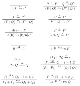
a.P−→ Pa P−→ Pa ′ Q a −→ Q′ (P | Q)−→ (Pτ ′| Q′) P−→ Pα ′ (P | Q)−→ (Pα ′| Q) P −→ Pα ′ P + Q−→ Pα ′ A(a) = P A(b)−→ [b/a]Pτ P −→ Pα ′ P ⊲ Q−→ Pα ′
0−−→ 0tick a.P −−→ a.Ptick P 6−→ ·τ P ⊲ Q−−→ Qtick (P1| P2) 6 τ −→ · Pi tick −−→ Qi i = 1, 2 (P1| P2) tick −−→ (Q1| Q2) Pi tick −−→ Qi i = 1, 2 P1+ P2 tick −−→ Q1+ Q2 P−→ Qµ a, a 6= µ νa P −→ νa Qµ
Table 1: Labelled transition system
where we write P −→ · if P can perform an action µ. TCCS is designed so that if P is aµ process built with the usual CCS operators and P cannot perform τ actions then P −−→ P .tick In other terms, CCS processes are time insensitive. To compensate for this property, one introduces a new binary operator P ⊲ Q, called else next, that tries to run P in the current instant and, if it fails, runs Q in the following instant.
We assume countably many names a, b, . . . For each name a there is a communication action a and a co-action a. We denote with α, β, . . . the usual CCS actions which are composed of either an internal action τ or of a communication action a, a, . . .. We denote with µ, µ′, . . .
either an action α or the distinct action tick.
The TCCS processes P, Q, . . . are specified by the following grammar P ::= 0 || a.P || P + P || P | P || νa P || A(a) || P ⊲ P .
We denote with fn(P ) the names free in P . We adopt the usual convention that for each thread identifier A there is a unique defining equation A(b) = P where the parameters b include the names in fn(P ). The related labelled transition system is specified in table 1.
Say that a process is a CCS process if it does not contain the else next operator. The reader can easily verify that:
(1) P −−→ · if and only if P 6tick −→ ·.τ
(2) If P −−→ Qtick ifor i = 1, 2 then Q1 = Q2. One says that the passage of time is deterministic.
(3) If P is a CCS process and P −−→ Q then P = Q. Hence CCS processes are closed undertick labelled transitions.
It will be convenient to write τ.P for νa (a.P | a.0) where a /∈ fn(P ), tick.P for 0 ⊲ P , and Ω for the diverging process τ.τ. . . ..
Remark 1 (1) In the labelled transition system in table 1, the definition of the tick action relies on the τ action and the latter relies on the communication actions a, a′, . . .. There is
a well known method to give a direct definition of the τ action that does not refer to the communication actions. Namely, one defines (internal) reduction rules such as (a.P + Q | a.P′+ Q′) → (P | P′) which are applied modulo a suitable structural equivalence.
(2) The labelled transition system in table 1 relies on negative conditions of the shape P 6−→.τ These conditions can be replaced by a condition ∃ L P ↓ L, where L is a finite set of commu-nication actions. The predicate ‘↓’ can be defined as follows:
0 ↓ ∅ a.P ↓ {a} Pi↓ Li, i = 1, 2 (P1+ P2) ↓ L1∪ L2 P ↓ L P ⊲ Q ↓ L P ↓ L (νa P ) ↓ L\{a, a} Pi↓ Li, i = 1, 2 L1∩ L2= ∅ (P1| P2) ↓ L1∪ L2
1.1 Signals and a deterministic fragment
As already mentioned, the TCCS model has been inspired by the notion of time available in the Esterel model [4] and its relatives such as SL [5]. These models rely on signals as the basic communication mechanism. Unlike a channel, a signal persists within the instant and disappears at the end of it. It turns out that a signal can be defined recursively in TCCS as:
emit(a) = a.emit(a) ⊲ 0
The ‘present’ statement of SL that either reads a signal and continues the computation in the current instant or reacts to the absence of the signal in the following instant can be coded as follows:
present a do P else Q = a.P ⊲ Q
Modulo these encodings, the resulting fragment of TCCS is specified as follows: P ::= 0 || emit(a) || present a do P else P || (P | P ) || νa P || A(a) .
Notice that, unlike in (T)CCS, communication actions have an input or output polarity. The most important property of this fragment is that its processes are deterministic [5, 1].
1.2 The usual labelled bisimulation
As usual, one can define a notion of weak transition as follows:
µ
⇒= (
(−→)τ ∗ if µ = τ
(−→)τ ∗◦−→ ◦(µ −→)τ ∗ otherwise
where the notation X∗ stands for the reflexive and transitive closure of a binary relation X.
When focusing just on internal reduction, we shall write → for −→ and ⇒ forτ ⇒. We writeτ P → · if ∃ P′ (P → P′), otherwise we say that P has converged and write P ↓. We write P ⇓
if ∃ Q (P ⇒ Q and Q ↓). Thus P ⇓ means that P may converge, i.e., there is a reduction sequence to a process that has converged. Because P ↓ iff P −−→ ·, we have that P ⇓ ifftick P tick⇒ ·.
With respect to the notion of weak transition, one can define the usual notion of bisimu-lation as the largest symmetric rebisimu-lation R such that if (P, Q) ∈ R and P ⇒ Pµ ′ then for some
Q′, Q ⇒ Qµ ′ and (P′, Q′) ∈ R. We denote with ≈u the largest labelled bisimulation (u for usual). When looking at CCS processes, one may focus on CCS actions (thus excluding the tick action). We denote with ≈u
ccs the resulting labelled bisimulation.
1.3 CCS vs. TCCS
As we already noticed, TCCS has been designed so that CCS can be regarded as a transition closed subset of TCCS. A natural question is whether two CCS processes which are equivalent with respect to an untimed environment are still equivalent in a timed one. For instance, Milner [9] discusses a similar question when comparing CCS to SCCS.2
1.3.1 Testing semantics
In the context of TCCS and of a testing semantics, the question has been answered negatively by Hennessy and Regan [6]. For instance, they notice that the processes P = a.(b + c.b) + a.(d + c.d) and Q = a.(b + c.d) + a.(d + c.b) are ‘untimed’ testing equivalent but ‘timed’ testing inequivalent. The relevant test is the one that checks that if an action b cannot follow an action a in the current instant then an action b will happen in the following instant just after an action c (process P will not pass this test while process Q does). This remark motivated the authors to develop a notion of ‘timed’ testing semantics.
1.3.2 Bisimulation semantics
What is the situation with the usual labelled bisimulation semantics recalled in section 1.2? Things are fine for reactive processes which are defined as follows.
Definition 2 A process P is reactive if whenever P µ1
⇒ · · · µn
⇒ Q, for n ≥ 0, we have the property that all sequences of τ reductions starting from Q terminate.
Proposition 3 Suppose P, Q are CCS reactive processes. Then P ≈u Q if and only if P ≈u ccs
Q.
Proof. Clearly, ≈u is a CCS bisimulation, hence P ≈u Q implies P ≈u
ccs Q. To show the
converse, we prove that ≈u
ccsis a timed bisimulation. So suppose P ≈uccsQ and P tick ⇒ P′. This means P ⇒ Pτ 1 tick −−→ P1 τ
⇒ P′. Then for some Q 1, Q
τ
⇒ Q1 and P1 ≈uccs Q1. Further, because
Q1 is reactive there is a Q2 such that Q1 τ
⇒ Q2 and Q2 ↓. By definition of bisimulation and
the fact that P1 ↓, we have that P1 ≈uccsQ2. So for some Q′, Q2 τ
⇒ Q′ and P′ ≈u
ccsQ′. Thus
we have shown that there is a Q′ such that Qtick⇒ Q′ and P′ ≈u
ccsQ′. 2
Proposition 3 fails when we look at non-reactive processes. For instance, 0 and Ω are regarded as untimed equivalent but they are obviously timed inequivalent since the second
2
The notion of instant in SCCS is quite different from the one considered in TCCS/Esterel. In the former one declares explicitly what each thread does at each instant while in the latter the duration of an instant is the result of an arbitrarily complex interaction among the different threads.
process does not allow time to pass. This example suggests that if we want to extend propo-sition 3 to non-reactive processes, then the notion of bisimulation has to be convergence sensitive.
One possibility could be to adopt the usual bisimulation ≈uon CCS processes. We already noticed that if P is a CCS process and P −−→ Q then P = Q. Thus in the bisimulation gametick between CCS processes, the condition ‘P tick⇒ P′ implies Q tick⇒ Q′’ can be replaced by ‘P ⇓
implies Q ⇓’. The resulting equivalence on CCS processes is not new, for instance it appears in [8] as the so called stable weak bisimulation. One may notice that this equivalence has reasonably good congruence properties.
Proposition 4 Suppose P1≈u P2 and Q1 ≈u Q2. Then
(1) (P1| R) ≈u(P2 | R).
(2) If P1, P2 ↓ then P1⊲ Q1 ≈uP2⊲ Q2.
Proof. First note that we can work with an asymmetric definition of bisimulation where a strong transition is matched by a weak one.
(1) We just check the condition for the tick action. Suppose (P1 | R) tick −−→ (P′ 1 | R′). This entails P1 tick −−→ P′ 1 and R tick −−→ R′. Then P 2 τ ⇒ P′′ 2, P2′′↓, and P1 ≈u P1′′. Also P2′′ tick ⇒ P′ 2 and P′
1 ≈u P2′′. Finally, we have that (P2′′ | R) ↓ because if they could synchronise on a name a
then so could (P1 | R).
(2) There are two cases to consider. If P1⊲ Q1 tick −−→ Q1 then P2⊲ Q2 tick −−→ Q2. If P1⊲ Q1 a − → P′ 1 because P1 a − → P′ 1 then P2 a ⇒ P′ 2 and P1′ ≈uP2′. 2
Remark 5 The else next operator suffers from the same compositionality problems as the sum operator. For instance, 0 ≈u τ.0 but 0 ⊲ Q = tick.Q while τ.0 ⊲ Q ≈u 0. As for the sum
operator, one may remark that in practice we are interested in a guarded form of the else next operator. Namely, the else next operator is only introduced as an alternative to a communi-cation action (the present operator discussed in section 1.1 is such an example). Proposition 4(2) entails that in this form, the else next operator preserves bisimulation equivalence.
1.3.3 An alternative path
The reader might have noticed that on CCS processes ≈u refines ≈u
ccs by adding may
con-vergence as an observable along with the usual labelled transitions. This is actually the case of all convergence/divergence sensitive bisimulations we are aware of (see, e.g., [15, 8]). The question we wish to investigate is: what happens if we just take may convergence as an ob-servable without assuming the observability of the labelled transitions? The question can be motivated by both pragmatic and mathematical considerations. On the pragmatic side, one may argue that the normal operation of a timed/synchronous program is to receive inputs at the beginning of each instant and to produce outputs at the end of each instant. Thus, unless the instant terminates, no observation is possible. For instance, the process (a | Ω) could be regarded as equivalent to Ω, while they are distinguished by the usual bisimulation ≈u on the
ground that the labelled transition a is supposed to be directly observable.
On the mathematical side, it has been remarked by many authors that the notion of labelled transition system is not necessarily compelling. Specifically, one would like to define a notion of bisimulation without an a priori commitment to a notion of label. To cope with
this problem, a well-known approach started in [11] and elaborated in [7] is to look at ‘internal’ reductions and at a basic notion of ‘barb’ and then to close under contexts thus producing a notion of ‘contextual’ bisimulation. However, even the notion ‘barb’ is not always easy to define and justify (an attempt based on the concept of bi-orthogonality is described in [13]). It seems to us that a natural approach which applies to a wide variety of formalisms is to regard convergence (may-termination) as the ‘intrinsic’ basic observable automatically provided by the internal reduction relation.
1.3.4 Contribution
Following these preliminary considerations, we are now in a position to describe our contri-bution.
1. We introduce a notion of contextual bisimulation for CCS whose basic observable (or barb) is the may-termination predicate (section 2).
2. We provide various characterisations of this equivalence culminating in one based on a suitable ‘convergence-sensitive’ labelled bisimulation (section 3).
3. We derive from this characterisation that (section 4):
(a) the embedding of CCS in TCCS is fully abstract (even for non-reactive processes). (b) the proposed equivalence coincides with the usual one on reactive processes.
(c) on non-reactive processes it identifies more processes than the usual timed labelled bisimulation ≈u.
(d) on non-reactive CCS processes it is incomparable with the usual labelled CCS bisimulation ≈u
ccs.
4. We refine the proposed notion of contextual bisimulation by making it sensitive to divergence and show that the characterisation results mentioned above can be extended to this case (section 5).
The development will take place in the context of so called weak bisimulation [10] which is more interesting and challenging than strong bisimulation.
2
Convergence sensitive bisimulation
We denote with C, D, . . . one hole static contexts specified by the following grammar: C ::= [ ] || C | P || νaC
We require that the notion of bisimulation we consider is preserved by the static contexts in the sense of [7].
Definition 6 (bisimulation) A symmetric relation R on processes is a bisimulation if P RQ implies:
cxt for any static context C, C[P ]RC[Q].
We denote with ≈ the largest bisimulation.
Remark 7 (1) In view of remark 1(1), the definition 6 of bisimulation does not assume the labels a, a′, . . . which correspond to the communication action. Not only the labels are not
considered in the bisimulation game, but they are not even required in the definition of the τ action. This means that the definition can be directly transferred to more complex process calculi where the definition of communication action is at best unclear.
(2) For CCS processes, if P −−→ Q then P = Q. It follows that in the definition above, thetick condition [red] when µ = tick can be replaced by P ⇓ implies Q ⇓. This is obviously false for processes including the else next operator; in this case one needs the tick action to observe the behaviour of processes after the first instant, e.g., to distinguish tick.a from tick.b.
In view of the previous remark, the definition of bisimulation is specialised to CCS pro-cesses by simply restricting the condition [cxt] to CCS static contexts. We denote with ≈ccs
the resulting largest bisimulation.
Next we remark that the observability of a ‘stable commitment (or barb)’ is entailed by the observation of convergence.
Definition 8 We say that P (stably) commits on a, and write P ⇓a, if P ⇒ P′, P′ ↓, and
P′ a−→ ·.3
Proposition 9 If P ≈ Q and P ⇓a then Q ⇓a.
Proof. Suppose P ⇓a and P ≈ Q. Then P ⇒ P′, P′ ↓, and P′ −→ ·. By definition ofa bisimulation, Q ⇒ Q′′ and P′≈ Q′′. Moreover, Q′′⇒ Q′, Q′ ↓, Q′ ≈ P′ ≈ Q′′. To show that Q′ a−→ ·, consider the context C = ([ ] | a.Ω). Then we have C[P′] 6⇓, while C[Q′] ⇓ if and only
if Q′ 6−→ ·.a
2 Another interesting notion is that of contextual convergence.
Definition 10 We say that a process P is contextual convergent, and write P ⇓C, if ∃ C (C[P ] ⇓
).
Clearly, P ⇓ implies P ⇓C but the converse fails taking, for instance, (a + b) | a.Ω.
Contextual convergence, can be characterised as follows. Proposition 11 The following conditions are equivalent: (1) P α1
−→ · · · αn
−−→ P′ and P′ ↓.
(2) There is a CCS process Q such that (P | Q) ⇓. (3) P ⇓C.
Proof. (1 ⇒ 2) Suppose P0 α1
−→ P1· · · αn
−−→ Pn and Pn ↓. We build the process Q in (2)
by induction on n. If n = 0 we can take Q = 0. Otherwise, suppose n > 0. By inductive hypothesis, there is Q1 such that (P1 | Q1) ⇓. We proceed by case analysis on the first action
α1. If α1= τ take Q = Q1 and if α1 = a take Q = a.Q1.
3
(2 ⇒ 3) Taking the static context C = [ ] | Q.
(3 ⇒ 1) First, check by induction on a static context C that P −→ · implies C[P ]τ −→ ·. Henceτ C[P ] ↓ implies P ↓. Second, show that C[P ] −→ Q implies that Q = Cα ′[P′] where C′ is a
static context and either P = P′ or P −→ Pα′ ′. Third, suppose C[P ] −→ Qτ 1· · ·
τ
−
→ Qn with
Qn ↓. Show by induction on n that P can make a series of labelled transitions and reach a
process which has converged. 2
Remark 12 As shown by the characterisation above, the notion of contextual convergence is unchanged if we restrict our attention to contexts composed of CCS processes.
We notice that a bisimulation never identifies a process which is contextual convergent with one which is not while identifying all processes which are not contextual convergent. Proposition 13 (1) If P ≈ Q and P ⇓C then Q ⇓C.
(2) If P 6⇓C and Q 6⇓C then P ≈ Q.
Proof. (1) If P ⇓C then for some context C, C[P ] ⇓. By condition [cxt], we have that C[P ] ≈ C[Q], and by condition [red] we derive that C[Q] ⇓. Hence Q ⇓C.
(2) We notice that the relation S = {(P, Q) | P, Q 6⇓C} is a bisimulation. Indeed: (i) if P 6⇓C
then C[P ] 6⇓C, (ii) if P ⇒ P′ and P 6⇓C then P′ 6⇓C, and (iii) if P 6⇓C then P 6 tick
⇒ ·. 2
3
Characterisation
We characterise the (contextual and convergence sensitive) bisimulation introduced in defini-tion 6 by means of a labelled bisimuladefini-tion. The latter is obtained from the former by replacing condition [cxt] with a suitable condition [lab] on labelled transitions as defined in table 1. Definition 14 (labelled bisimulation) A symmetric relation R on processes is a labelled bisimulation if P RQ implies:
lab if P ⇓C and P a
⇒ P′ then Q⇒ Qα ′ and P′RQ′ where α ∈ {a, τ } and α = a if P′⇓ C.
red if P ⇒ Pµ ′, µ ∈ {τ, tick} then ∃ Q′ (Q⇒ Qµ ′ and P′RQ′).
We denote with ≈ℓ the largest labelled bisimulation.
Remark 15 (1) By remark 7, on CCS processes the condition [red] when µ = tick is equiv-alent to: ‘P ⇓ implies Q ⇓’. By remark 12, the notion of contextual convergence is unaffected if we restrict our attention to CCS processes. This means that, by definition, the (timed) labelled bisimulation restricted to CCS processes is the same as the labelled bisimulation on (untimed) CCS processes.
(2) The predicate of contextual convergence ⇓C plays an important role in the condition [lab].
To see why, suppose we replace it with the predicate ⇓ and assume we denote with ≈ℓ⇓ the
resulting largest labelled bisimulation. The following example shows that ≈ℓ⇓ is not preserved
by parallel composition. Consider:
Then (P1 | Q) ≈ℓ⇓ (P2 | Q) because both processes fail to converge. On the other hand,
(P1 | Q) | d 6≈ℓ⇓(P2 | Q) | d because the first may converge to (b + c) which cannot be matched
by the second process.
(3) One may consider an asymmetric and equivalent definition of labelled bisimulation where strong transitions are matched by weak transitions. To check the equivalence, it is useful to note that P 6⇓C and P
α
−→ P′ implies P′6⇓ C.
We provide a rather standard proof that bisimulation and labelled bisimulation coincide. Proposition 16 If P ≈ Q then P ≈ℓ Q.
Proof. We show that the bisimulation ≈ is a labelled bisimulation. We denote with P ⊕ Q the internal choice between P and Q which is definable, e.g., as τ.P + τ.Q. Suppose P ⇓C
and P ⇒ Pa ′. We consider a context C = [ ] | T where T = a.((b ⊕ 0) ⊕ c) and b, c are ‘fresh
names’ (not occurring in P, Q). We know C[P ] ≈ C[Q] and C[P ] ⇒ (P′ | (b ⊕ 0)). Thus
C[Q] ⇒ (Q′ | T′) where either Q⇒ Qa ′ and T ⇒ Ta ′ or Q ⇒ Q′ and T = T′.
• Suppose P′ 6⇓
C. Then (P′ | (b ⊕ 0)) 6⇓C and, by proposition 13, (Q′ | T′) 6⇓C. The
latter implies that Q′ 6⇓
C. By contradiction, suppose Q′ ⇓C, that is (Q′ | R) ⇓. Then
(Q′ | T′) | R | T′ ⇓ (contradiction!), where we take T′ = a if T′ = T and T′ = 0 otherwise.
Hence, P′ ≈ Q′ as required.
• Suppose P′ ⇓ C. If Q
a
⇒ Q′ and T ⇒ Ta ′ then we show that it must be that T′ = (b⊕0). This
is because if P′ ⇓
C then P′ | (b ⊕ 0) ⇓C which in turn implies that for some R (not containing
the names b or c), (P′ | (b ⊕ 0) | R) ⇓
b. By proposition 9, we must have Q′′= (Q′ | T′) | R ⇓b.
Thus T′cannot be 0 and it cannot be (b⊕0)⊕c, for otherwise Q′′⇓
cwhich cannot be matched
by (P′ | (b⊕0) | R). Further, we have P′ | (b⊕0)−→ Pτ ′ | 0 (= P′). So (Q′ | (b⊕0))⇒ (Qτ ′ | T′′)
and P′ ≈ (Q′ | T′′). The latter entails that T′′= 0.
On the other hand, we show that Q⇒ Qτ ′ and T = T′ is impossible. Reasoning as above,
we have (P′ | (b ⊕ 0) | R) ⇓
b. But then if (Q′ | T ) | R ⇓b we shall also have (Q′ | T ) | R ⇓c. 2
The following lemma relates contextual convergence to labelled bisimulation (cf. the similar proposition 13).
Lemma 17 (1) If P ≈ℓQ and P ⇓
C then Q ⇓C.
(2) If P 6⇓C and Q 6⇓C then P ≈ℓQ.
Proof. (1) By proposition 11, if P ⇓C then P α1
−→ · · · αn
−−→ P′ and P′ ↓. By definition of
labelled bisimulation we should have Q α1
⇒ · · · αn
⇒ Q′ and P′ ≈ℓ Q′. Then P′ tick⇒ · entails
Q′ tick⇒, and therefore Q ⇓ C.
(2) By proposition 13, P, Q 6⇓C implies P ≈ Q, and by proposition 16 we conclude that
P ≈ℓQ.
2 Proposition 18 If P ≈ℓQ then P ≈ Q.
Proof. We show that labelled bisimulation is preserved by static contexts. In view of remark 15(3), we shall work with an asymmetric definition of bisimulation. With respect to this definition, we show that the following relations are labelled bisimulations:
{(νa P, νa Q) | P ≈ℓQ}∪ ≈ℓ , {(P | R, Q | R) | P ≈ℓQ}∪ ≈ℓ .
The case for restriction is a routine verification so we focus on parallel composition. Suppose (P | R)−→ ·. We proceed by case analysis.µ
• (P | R)−→ (P | Rα ′) because R−→ Rα ′. Then (Q | R)−→ (Q | Rα ′).
• (P | R)−−→ (Ptick ′ | R′) because P −−→ Ptick ′ and R−−→ Rtick ′. Then Q ⇒ Q 1
tick
−−→ Q2 ⇒ Q′ and
P′ ≈ℓ Q′. Notice that P ≈ℓ Q
1 with P, Q1 ↓, and therefore (Q1 | R) tick −−→ (Q2 | R′). Hence (Q | R)tick⇒ (Q′ | R′). • Suppose (P | R) ⇓C and (P | R) a −→ (P′ | R) because P −→ Pa ′. Then P ⇓ C and therefore Q⇒ Qα ′, α ∈ {a, τ }, and P′ ≈ℓQ′. If (P′| R) ⇓
C then P′ ⇓C and this entails α = a.
• Suppose (P | R)−→ (Pτ ′| R) because P −→ Pτ ′. Then Q⇒ Qτ ′ and P′ ≈ℓQ′.
• Suppose (P | R) −→ (Pτ ′ | R′) because P → P−a ′ and R −→ Ra ′. If P, P′ ⇓
C then Q a ⇒ Q′ and P′ ≈ℓ Q′. If P ⇓ C and P′ 6⇓C then Q α
⇒ Q′, α ∈ {a, τ }, and P′ ≈ℓ Q′. But then
(P′ | R), (Q′ | R) 6⇓
C, and we apply lemma 17. If P 6⇓C then Q 6⇓C and therefore (Q | R) 6⇓C,
and we apply again lemma 17. 2
As a first application of the characterisation we check that bisimulation is preserved by the else next operator in the sense of proposition 4(2).
Corollary 19 Suppose P1 ≈ P2, P1, P2 ↓, and Q1 ≈ Q2. Then P1⊲ Q1 ≈ P2⊲ Q2.
Proof. There are two cases to consider. If P1 ⊲ Q1 tick −−→ Q1 then P2 ⊲ Q2 tick −−→ Q2. If P1⊲ Q1 a − → P′ 1 because P1 a − → P′ 1 then P2 α ⇒ P′
2, P1′ ≈ℓ P2′, and α ∈ {τ, a}. We note that it
must be that α = a. Indeed, if α = τ then since P2 ↓ we must have P2′ = P2 and P1′ ⇓C. The
latter forces α = a which is a contradiction. 2
4
Embedding CCS in TCCS
In this section we collect some easy corollaries of the characterisation. First, we remark that two CCS processes are bisimilar when observed in an untimed/asynchronous environment if and only if they are bisimilar in a timed/synchronous environment.
Proposition 20 Suppose P, Q are CCS processes. Then P ≈ Q if and only if P ≈ccs Q.
Proof. By propositions 16 and 18 we know that ≈=≈ℓ. By remark 15(1), the labelled bisimulation on untimed processes coincides with the restriction to CCS processes of the
timed labelled bisimulation. 2
Second, we compare the notion of convergence-sensitive bisimulation we have introduced with the usual one we have recalled in the section 1.2. All the notions collapse on reactive processes.
Proposition 21 Suppose P, Q are reactive processes. Then P ≈ Q if and only if P ≈u Q.
Proof. We know that ≈=≈ℓ. Reactive processes are closed under labelled transitions and on reactive processes the conditions that define labelled bisimulation coincide with the ones
for the usual bisimulation. 2
The situation on non-reactive processes is summarised as follows where all implications are strict.
Proposition 22 Suppose P, Q are processes. (1) If P ≈u Q then P ≈ Q.
(2) If moreover P and Q are CCS processes then P ≈uQ implies both P ≈u
ccsQ and P ≈ Q.
Proof. (1) The clauses in the definition of ≈u imply directly those in the definition of the labelled bisimulation that characterises ≈ (definition 14). To see that the converse fails note that (a | Ω) ≈ Ω while (a | Ω) 6≈uΩ.
(2) Use (1) and the fact that the clauses in the definition of ≈u imply directly those in the definition of ≈u
ccs. To see that the converse fails use the counter-example in (1) and the fact
that 0 ≈u
ccsΩ while 0 6≈u Ω. 2
5
Divergence sensitive bisimulation
We refine the notion of bisimulation to make it sensitive to divergence and show that the characterisation presented in section 3 can be adapted to this case.
We say that a process P may diverge and write P ⇑ if there is an infinite reduction sequence of τ actions that starts from P . We refine the notion of bisimulation by making it sensitive to divergence.
Definition 23 (⇑-bisimulation) A symmetric relation R on processes is a divergence sen-sitive bisimulation (⇑-bisimulation, for short) if it is a bisimulation according to definition 6 and if P RQ and P ⇑ implies Q ⇑. We denote with ≈⇑ the largest ⇑-bisimulation.
Remark 24 Say that a process P is strongly normalising if all reduction sequences of τ -actions that start from P terminate. A process is strongly normalising if and only if it may not diverge. It follows that one can give an equivalent formulation of ⇑-bisimulation by replacing the may divergence predicate with the strong normalisation predicate.
We notice the following properties whose proof is direct. Proposition 25 (1) If P ≈⇑Q then P ≈ Q.
(2) If P ≈⇑Q and P ⇓a then Q ⇓a.
(3) If P ≈⇑Q and P ⇓C then Q ⇓C.
(4) If P 6⇓C then P ⇑.
Proof. (1) A ⇑-bisimulation is also a bisimulation. (2) We apply (1) and proposition 9.
(3) We apply (1) and proposition 13(1). (4) Immediate, by definition.
(5) If P 6⇓C and Q 6⇓C then P ⇑ and Q ⇑. 2
It follows that ⇑-bisimulation coincides with bisimulation on the processes that are not contextual convergent. On the other hand, on those that are contextual convergent, it is a strictly finer notion as, e.g., it distinguishes 0 from A = τ.A + τ.0.
The characterisation of ⇑-bisimulation turns out to be straightforward: it is enough to make the labelled bisimulation we have introduced in definition 14 sensitive to divergence. Definition 26 (⇑-labelled bisimulation) A symmetric relation R on processes is a diver-gence sensitive labelled bisimulation (or ⇑-labelled bisimulation) if it is a labelled bisimulation and if P RQ and P ⇑ implies that Q ⇑. We denote with ≈ℓ
⇑ the largest ⇑-labelled bisimulation.
Because of the properties stated in proposition 25, one can repeat the proofs in section 3 while adding specific arguments to take the sensitivity to divergence into account.
Proposition 27 If P ≈⇑Q then P ≈ℓ⇑Q.
Proof. We show that ≈⇑ is a ⇑-labelled bisimulation by repeating the proof schema in proposition 16. Note that the condition that refers to divergence is the same for ⇑-bisimulation
and for ⇑-labelled bisimulation. 2
Lemma 28 (1) If P ≈ℓ
⇑Q and P ⇓C then Q ⇓C.
(2) If P 6⇓C and Q 6⇓C then P ≈ℓ⇑Q.
Proof. (1) Note that P ≈ℓ
⇑Q implies P ≈ℓQ and apply lemma 17(1).
(2) By proposition 25(5), P 6⇓C and Q 6⇓C implies P ≈⇑Q and by proposition 27 the latter
implies P ≈ℓ
⇑Q. 2
Proposition 29 If P ≈ℓ
⇑Q then P ≈⇑Q.
Proof. As in proposition 18, we have to verify that ≈ℓ
⇑ is preserved by name generation and
parallel composition. For the former we note that νa P ⇑ if and only if P ⇑. For the latter, we can repeat the proof in proposition 18. Moreover, we have to consider the case where P ≈ℓ
⇑Q
and (P | R) ⇑. The process (P | R) diverges because: either P and R may engage in a finite number of synchronisations after which one of the two diverges or P and R may engage in an infinite number of synchronisations. Suppose the finite or infinite number of synchronisations between P and R correspond to the transitions P a1
⇒ P1 a2 ⇒ · · · and R a1 ⇒ R1 a2 ⇒ · · · If P, P1, · · ·
are all contextually convergent then Q a1
⇒ Q1 a2
⇒ · · · and Pi≈ℓ⇑Qi. Hence (Q | R) ⇑. If P 6⇓C
then Q 6⇓C implies (Q | R) 6⇓C which implies (Q | R) ⇑. Finally, suppose Pi is the least i
such that Pi 6⇓C. Then Q a1
⇒ · · · a⇒ Qi−1 i−1 αi
⇒ Qi with Qi 6⇓C and αi ∈ {ai, τ }. If αi = ai
then (Q | R) ⇑ because (Q | R) ⇒ (Qτ i | R′) and Qi ⇑. If αi = τ then (Q | R) ⇑ because
6
Conclusion
We have presented a natural notion of contextual and convergence sensitive bisimulation and we have shown that it can be characterised by a variant of the usual notion of labelled bisimulation relying on the concept of contextual convergence. As a direct corollary of this characterisation, we have shown that (untimed) CCS processes are embedded fully abstractly into timed ones. Finally, we have refined the notion of bisimulation to make it divergence-sensitive.
We believe that our main contribution, if any, is of a methodological nature. The notion of bisimulation we have introduced just requires the notions of reduction and static context as opposed to previous approaches that build on the notion of ‘labelled’ transition or on the notion of ‘barb’. It would be interesting to apply the proposed approach to other situations where the notion of equivalence is unclear. For instance, we expect that our results can be extended to a TCCS with ‘asynchronous’ communication or with ‘signal-based’ communica-tion.
References
[1] R. Amadio. The SL synchronous language, revisited. Journal of Logic and Algebraic Programming, 70:121-150, 2007.
[2] R. Amadio. A synchronous π-calculus. Information and Computation, 205(9):1470–1490, 2007.
[3] G. Berry, L. Cosserat. The Esterel synchronous programming language and its mathe-matical semantics. INRIA technical report 842, Sophia-Antipolis, 1988.
[4] G. Berry and G. Gonthier. The Esterel synchronous programming language. Science of computer programming, 19(2):87–152, 1992.
[5] F. Boussinot and R. De Simone. The SL synchronous language. IEEE Trans. on Software Engineering, 22(4):256–266, 1996.
[6] M. Hennessy, T. Regan. A process algebra of timed systems. Information and Compu-tation, 117(2):221-239, 1995.
[7] K. Honda and N. Yoshida. On reduction-based process semantics. Theoretical Computer Science, 151(2):437-486, 1995.
[8] M. Lohrey, P. D’Argenio, and H. Hermanns: Axiomatising divergence. In Proc. ICALP, SLNCS 2380:585-596, 2002.
[9] R. Milner. Calculi for synchrony and asynchrony. Theoretical Computer Science, 25(3):267–310, 1983.
[10] R. Milner. Communication and Concurrency. Prentice-Hall, 1989.
[11] R. Milner and D. Sangiorgi. Barbed bisimulation. In Proc. ICALP, SLNCS 623:685–695, 1992.
[12] X. Nicolin, J. Sifakis. The algebra of timed processes (ATP): theory and application. Information and Computation, 114(1):131-178, 1994.
[13] J. Rathke, V. Sassone and P. Sobocinski. Semantic barbs and biorthogonality. In Proc. FoSSaCS 2007, SLNCS 4423:302-316, 2007.
[14] W. Yi. A calculus of real time systems. PhD thesis. Chalmers University, 1991.
[15] D. Walker. Bisimulation and divergence. Information and Computation, 85:202-241, 1990.