HAL Id: hal-01922719
https://hal.inria.fr/hal-01922719
Submitted on 14 Nov 2018
HAL is a multi-disciplinary open access
archive for the deposit and dissemination of sci-entific research documents, whether they are pub-lished or not. The documents may come from teaching and research institutions in France or abroad, or from public or private research centers.
L’archive ouverte pluridisciplinaire HAL, est destinée au dépôt et à la diffusion de documents scientifiques de niveau recherche, publiés ou non, émanant des établissements d’enseignement et de recherche français ou étrangers, des laboratoires publics ou privés.
Population-based priors in cardiac model personalisation
for consistent parameter estimation in heterogeneous
databases
Roch Molléro, Xavier Pennec, Hervé Delingette, Nicholas Ayache, Maxime
Sermesant
To cite this version:
Roch Molléro, Xavier Pennec, Hervé Delingette, Nicholas Ayache, Maxime Sermesant. Population-based priors in cardiac model personalisation for consistent parameter estimation in heterogeneous databases. International Journal for Numerical Methods in Biomedical Engineering, John Wiley and Sons, 2019, 35 (2), pp.e3158. �10.1002/cnm.3158�. �hal-01922719�
DOI: xxx/xxxx
Population-Based Priors in Cardiac Model Personalisation for
Consistent Parameter Estimation in Heterogeneous Databases
Roch Molléro | Xavier Pennec | Hervé Delingette | Nicholas Ayache | Maxime Sermesant*
1Inria, Epione Research Project, Sophia
Antipolis, France
Correspondence
Email: [email protected]
Personalised cardiac models are a virtual representation of the patient heart, with parameter values for which the simulation fits the available clinical measurements. Models usually have a large number of parameters while the available data for a given patient is typically limited to a small set of measurements, thus the parameters can-not be estimated uniquely. This is a practical obstacle for clinical applications, where accurate parameter values can be important. Here we explore an original approach based on an algorithm called Iteratively Updated Priors (IUP), in which we perform successive personalisations of a full database through Maximum A Posteriori (MAP) estimation, where the prior probability at an iteration is set from the distribution of personalised parameters in the database at the previous iteration. At the convergence of the algorithm, estimated parameters of the population lie on a linear subspace of reduced (and possibly sufficient) dimension in which for each case of the database, there is a (possibly unique) parameter value for which the simulation fits the mea-surements. We first show how this property can help the modeler select a relevant parameter subspace for personalisation. In addition, since the resulting priors in this subspace represent the population statistics in this subspace, they can be used to perform consistent parameter estimation for cases where measurements are possibly different or missing in the database, which we illustrate with the personalisation of a heterogeneous database of 811 cases.
KEYWORDS:
Cardiac Electromechanical Modeling, Parameter Estimation, Parameter Selection, Personalised modeling
1
INTRODUCTION
Personalised cardiac models are of increasing interest for clin-ical applications13,1,22. To that end, parameter values of a cardiac model are estimated to get a personalised simula-tion which reproduces the available measurements for a clin-ical case. Then the personalised simulations can be used for advanced analysis of pathologies. In particular, recent works have been successful in predicting haemodynamic changes in cardiac resynchronization therapy21, ventricular tachycar-dia inducibility and dynamics6, as well as in detecting and localising infarcts8using 3D personalised models.
Most cardiac models depend on many parameters, espe-cially in 3D models where each parameter can take a different value at each node or region of the mesh,16,13,2,9. The num-ber of parameters can be up to tens of thousands while on the other hand for an individual patient, the available clinical data is usually sparse and typically consists of a set of global measurements (such as ejection fraction, systolic and diastolic pressure) and possibly some imaging data with a consider-able degree of noise or blurriness. Consequently, many sets of parameter values can lead to a simulation which can reproduce the available clinical data. The parameter estimation problem is an ill-posed inverse problem and all the parameters cannot be uniquely estimated from the measurements only.
A classic technique to estimate relevant parameters in this context is the use of prior probabilities distributions over the parameter values19,14,15. In this framework, parameters values come from a (usually Gaussian) prior probability distribution, which represents some knowledge or beliefs about the distri-bution of parameters. Then, given a set of measurements, a vector of Maximum A Posteriori (MAP) parameter values is estimated, which realises an optimal trade-off between its like-lihood in the prior probability distribution and the error of fit of the simulation. The set of Maximum A Posteriori values is usually smaller than the set of values for which the simulation fits the measurements and possibly unique. A challenge to esti-mate relevant parameters is then to define accurately the prior
probability distribution, which should be ideally as close as possible to the "true" distribution of parameters.
Here we explore an original approach which we call
Iter-atively Updated Priors (IUP), to adress the chicken-and-egg
problem of defining an accurate “prior” when not other infor-mation is available beside the currently considered data. It consists in performing successive personalisations with pri-ors, where the priors distribution is set from the distribution of personalised parameters in the previous personalisation. The rationale is twofold: first, if the algorithm converges, all the cases are personalised through a MAP where the prior distribu-tion is the distribudistribu-tion of the populadistribu-tion parameters itself. Intu-itively this opens the possibility, for cases where the value of a parameter is unobservable, to regularise the fitting by using
population informationfrom other cases in the database where the value was observable. Secondly, when there are directions in the parameter space in which the simulated measurements do not vary (i.e. an unobservable parameter direction), the use of priors promotes the estimation of parameter values which are closer to the prior mean, which in turn makes the penalty (from the prior) stronger in this direction at the next personal-isation. Intuitively, this process will tend to group parameters onto directions which are observable, and reduce the spread into directions which are not. In practice, we will see this algorithm leads the parameters to lie on a linear subspace of smaller dimension (See Figure 1 ).
In Section 2 we present the IUP algorithm in relation to two different mathematical tools. First, we express parameter esti-mation as a Maximum A Posteriori (MAP) estiesti-mation with prior probability distributions. Secondly, we use the Iteratively
Reweighted Least Square (IRLS)algorithm from sparse regres-sion to show that the IUP algorithm, when it converges, per-forms the minimisation of population-wide cost function with a sparse regulariser on the number of dimensions of the
parame-ter space. We introduce two types of updates of the parameters of the (Gaussian) prior probability: "Full Matrix", where no assumption is made on the distribution and the covariance matrix, and "Diagonal Matrix" where the covariance matrix
is supposed diagonal, which assumes independence of param-eters in the distribution of the population. We demonstrate that in the first case the algorithm leads to the automatic selection of parameter directions in which parameter values are set to a constant value in the population, and in the second case to the automatic selection of parameters which are set constant.
In Section 3 we present results of the IUP algorithm on a database of 137 complete cases where the same 4 measure-ments are available. We perform the estimation of 6 parameters of a cardiac model likely to vary in this population, which also makes the problem ill-conditioned. We observe that the IUP algorithm leads to a trade-off between the number of dimen-sions of the final parameter set, and the mean error of fit of the 4 measurements across the whole database of personalised simulations. Then we show that if we impose a high good-ness of fit of the personalised simulations, the algorithm leads to the selection of a linear subspace of minimal dimension in which for each case of the database there are parameter values where the simulation fits exactly the measurements. We dis-cuss how this algorithm can be used to find a relevant subspace for personalisation from the modeling point of view. Finally we extract a relevant subspace of dimension 4, based on 5 param-eters out of the original 6, in which there is a unique set of parameter values for each case of the database.
In the last section we apply the proposed framework to the consistent personalisation of a larger database of 811 cases, in which the set of measurements reported by the clinicians are heterogeneous and sometimes incomplete. Applied to this database, the algorithm leads to personalised simulations with high goodness of fit for all the cases of the population while grouping the parameters onto a parameter space of minimal dimension. Simultaneously, the resulting population-based
priors computed in this parameter space lead to consistent parameter estimation for the cases where the parameters are not all observable, and are in particular influenced by their values in cases of the population where they are observable. Finally we show how external parameters such as the weight and the height of the patient can also be added to the prior distribu-tion in order to constrain the parameter estimadistribu-tion with more consistency in case of unobservability.
2
ITERATIVELY UPDATED PRIORS AND
POPULATION-BASED PRIORS
In this section we introduce the personalisation framework, based on the estimation of a Maximum A Posteriori (MAP) with prior probabilities. In order to get relevant values for each case through MAP estimation, the prior probability has to be relevant. Ideally, it should be the "true" underlying probabil-ity distribution of parameters in the population. We introduce
FIGURE 1 Schematic representation (with synthetic data) of parameter estimation when the problem is ill-posed: in this
example both the contractility and the stiffness are estimated from values of the stroke volume (SV). Both have an influence on the stroke volume (SV) so there are isolines of stroke volume (in grey) on which the value of the stroke volume is the same.
Image a: estimation without priors, the estimated values (green) for each case can be anywhere on an isoline (grey). Image b:
the estimation is performed with a (gaussian) prior (the gaussian covariance is in blue), the estimated values are grouped closer to the prior mean. Image c: the Iteratively Updated Priors (IUP) algorithm performs successive estimations where the prior is set from the distribution of estimated parameters at the previous iteration. This leads the parameters to lie on a reduced linear
subspace(orange).
here the Iteratively Updated Priors (IUP) algorithm, which performs successive personalisations of the whole population, where the prior at each step is set from the distribution of the personalised parameters at the previous step.
First we present the MAP estimation of personalised param-eters or a single case (Section 2.1). Then we formulate the
Iteratively Updated Priorsalgorithm for a population of cases (Section 2.2). We then give the equations of the prior param-eter update in two different cases with different assump-tions on the shape of the distribution (Section 2.3) and the equations which are minimised within our optimisation frame-work (Section 2.4). Finally we present a link between the IUP algorithm and the Iteratively Reweighted Least Square algorithm for sparse regularisation, and show that the IUP algorithm performs the minimisation of a population-wide cost function with a penalty on the rank of the set of personalised parameters (Section 2.5). Finally we present a modification of the IUP algorithm called IUP* to impose a high goodness of
fit to the model outputs to the target values for each case and at each iteration (Section 2.6).
2.1
Maximum A Posteriori Estimation of
Personalised Parameters
We consider a cardiac model 𝑀 and a set of simulated quan-tities called the outputsO, such as the ejected volume and the mean ventricular pressure. We then consider a subsetPMof varying parameters (such as the contractility, the aortic resis-tance) of the model, while the other model parametersP′
M are supposed fixed. Given a vector 𝑥 of values of the param-etersPM, we noteOM(𝑥) the values of the outputsO of the model M.
With these notations, personalisation consists in estimat-ing parameter values 𝑋 for which the outputs valuesOM(𝑋) are consistent with some observed values ̂O of these outputs. This is an inverse problem, which can be tackled by different methods (see the review of Chabiniok et al.4).
A classic approach is to formulate the problem as the esti-mation of a Maximum A Posteriori with prior probabilities on the parameter values. With Bayes’ theorem, the posterior
prob-ability 𝑃(𝑥| ̂O) of parameter values considering the observed output values ̂O is proportional to the product of the
con-ditional likelihood 𝑃( ̂O|𝑥) and the prior probability 𝑃 (𝑥):
𝑃(𝑥| ̂O) ∝ 𝑃 ( ̂O|𝑥)𝑃 (𝑥) (1) In this work, we use Gaussian distributions for both the condi-tional likelihood and the prior probability:
{ 𝑃( ̂O|𝑥) ∝ 𝑒−12(𝑂(𝑥)− ̂𝑂) 𝑇Σ−1(𝑂(𝑥)− ̂𝑂) 𝑃(𝑥) ∝ 𝑒−12(𝑥−𝜇) 𝑇 Δ−1(𝑥−𝜇) (2)
which correspond to the assumptions that first, the observed values ̂𝑂are the sum of the outputs values 𝑂(𝑥) and a Gaussian noise with covariance Σ. Second, the underlying probablity distribution of the model parameters is a Gaussian with mean
𝜇and covarianceΔ. Finding a Maximum A Posteriori (MAP) consists in finding (one of) the parameter values which has the highest posterior probability:
𝑋= 𝑎𝑟𝑔𝑚𝑎𝑥𝑥𝑃(𝑥| ̂𝑂) (3)
This can also be interpreted as finding a maximum of the joint probability 𝑃(𝑥, ̂𝑂) of x and ̂𝑂with a uniform prior P( ̂𝑂) on ̂𝑂, thanks to the formula:
𝑃(𝑥, ̂𝑂) = 𝑃 (𝑥| ̂𝑂)𝑃 ( ̂𝑂) (4)
2.2
Iteratively Updated Priors (IUP)
In the following we consider a population of 𝑖 = 1..𝑛 cases to be personalised, we note ̂O = ( ̂𝑂1, ..., ̂𝑂𝑛) and
X = (𝑥1, ..., 𝑥𝑛). We introduce the algorithm called Iteratively
Updated Priors(IUP) which consists in successively estimat-ing personalised parameters 𝑋𝑖 with the MAP estimation, and re-estimating the prior parameters (𝜇, Δ) as the maxi-mum likelihood of these parameters considering the estimated personalised parameters 𝑋𝑖:
• Step 1: Personalisation
For each case i, find 𝑋𝑖 = 𝑎𝑟𝑔𝑚𝑎𝑥𝑥𝑖𝑃(𝑥𝑖, ̂𝑂𝑖|𝜇, Δ). This consists in performing the MAP estimation in Equation 3 for each case with current 𝜇 andΔ, which is the estimation of personalised parameters with a given prior.
• Step 2: Re-estimation of the Prior
Find(𝜇, Δ) = 𝑎𝑟𝑔𝑚𝑎𝑥(𝜇,Δ)𝑃(X|𝜇, Δ).
This consists in finding the most likely values (maxi-mum likelihood estimation) of 𝜇 andΔ given a set of personalised parametersX.
When the algorithm converges, the prior probability dis-tribution with the resulting parameters (𝜇∗,Δ∗) is called a
population-based priorbased on the ̂𝑂𝑖.
2.3
Explicit update formulas for 𝜇 and
Δ in
two cases.
We explicit here the update in the Step 2 of the IUP algorithm in which 𝜇 and Δ are set to the solutions of (𝜇, Δ) =
𝑎𝑟𝑔𝑚𝑎𝑥(𝜇,Δ)𝑃(X|𝜇, Δ). We consider two formulations of the Gaussian prior probability:
• First, a case (Full Matrix) where no assumptions are made on the covariance matrixΔ of the Gaussian distri-bution.
• Second, a case (Diagonal Matrix) where we suppose thatΔ is diagonal. This is equivalent to the (simplifying) assumption that parameter values are independent from each other in the population.
The solutions of the maximum likelihood estimation of 𝜇 and Δ in the two cases are1:
• Update of 𝜇: In both cases, 𝜇 is set to the mean of
personalised parameters 𝑋𝑖: 𝜇𝑘= 1 𝑛 𝑛 ∑ 𝑖=1 𝑋𝑖𝑘−1 (5)
• "Full Matrix" update ofΔ: In this case the minimisa-tion is reached whenΔ is the covariance matrix of the personalised parameters: Δ𝑘= 1 𝑛 𝑛 ∑ 𝑖=1 (𝑋𝑖𝑘−1− 𝜇𝑘)(𝑋𝑖𝑘−1− 𝜇𝑘)𝑇 (6)
• "Diagonal Matrix" update ofΔ: In this case the min-imisation is reached whenΔ is the diagonal part of the covariance matrix of the personalised parameters:
Δ𝑘= 𝐷𝑖𝑎𝑔(1 𝑛 𝑛 ∑ 𝑖=1 (𝑋𝑘−1 𝑖 − 𝜇 𝑘)(𝑋𝑘−1 𝑖 − 𝜇 𝑘)𝑇) (7)
2.4
Practical Implementation of the MAP
Estimation.
In the following, we use a constant Σ = 𝛾𝑑𝑖𝑎𝑔(N ) for the noise model in 2, whereN is a normalisation vector whose coefficients are explicited later.
1A practical derivation of the maximum likelihood estimation of the
covari-ance matrix can be found in https://people.eecs.berkeley.edu/ jordan/courses/260-spring10/other-readings/chapter13.pdf
We find the MAP of Equation 3 through the minimiza-tion of the negative log-likelihood −2
𝜆𝑙𝑜𝑔(𝑃 (𝑥| ̂𝑂), 𝜇, Δ), a
regularised cost-functionwhich we call ̂𝑆:
̂
𝑆(𝑥, ̂𝑂, 𝜇,Δ) = 𝑆(𝑥, ̂𝑂) + 𝛾𝑅(𝑥) (8)
with {
𝑅(𝑥) = (𝑥 − 𝜇)𝑇Δ−1(𝑥 − 𝜇)
𝑆(𝑥, ̂𝑂) =||(𝑂(𝑥) − ̂𝑂) ⊘N ||2 (9) where ⊘ is the Hadamard (coordinate-by-coordinate) division. We call 𝑆(𝑥, ̂𝑂) the data-fit term and 𝑅(𝑥) the regularisation
term.
We perform optimisation of this function with a derivative-free algorithm called CMA-ES11, which stands for Covariance Matrix Adaptation Evolution Strategy. It asks at each itera-tion 𝑛 for the scores of 𝑚 points 𝑥𝑖(a generation), drawn from
a multivariate distribution with covariance 𝐼𝑐
𝑛 and mean 𝐼 𝑚 𝑛.
Then, it combines Bayesian principles of maximum likelihood with natural gradient descent on the ranks of the points scores in the generation to update both 𝐼𝑛𝑐and 𝐼𝑛𝑚.
For each MAP estimation, we perform from 50 to (maxi-mum) 250 iterations of CMA-ES with a population size of 20, and the algorithm also stops if all the values of
√
̂
𝑆, (which we call the data-fit term) within the search space are in an interval smaller than 0.01.
The algorithm is stochastic (because the parameter values of the generation samples are drawn randomly). It iteratively enlarges its search space until it contains a minimal solution, then reduces the search space according to the best members of each generation (drawn randomly). As a consequence it does not converge to the same solution when the possible solu-tions are not unique. Because of this it can be used to give an (empirical) evaluation of the "non-uniqueness variability" by repeating the personalisation process multiple times.
Finally for practical reasons, since all the parameters of our model are positive, we always consider in the following the logarithm of parameter values instead of their values. This enables in particular to not have the optimisation algorithm test negative (non-physical) values in this step.
2.5
Link with Sparse Regularization
The IUP algorithm as presented in Section 2.2 has strong links with the Iteratively Reweighted Least Squares (IRLS) algorithm in sparse regression. When the IUP converges, we can show (see a more complete derivation in APPENDIX A) that it performs the minimization of a population-wide cost
function, with a penalty on the rank of the set of personalised
parameters: S(X, ̂O) = 1 𝑛 𝑛 ∑ 𝑖=1 𝑆(𝑥𝑖, ̂𝑂𝑖) + 𝛾𝐷 (10)
Where 𝐷 is the rank (number of non-zero eigenvalues) of Δ∗, which is the covariance of the set of personalised parame-ters at convergence. The minimisation of 𝐷 thus correspond to the minimisation of the number of dimensions of the set of
per-sonalised parameters. With the Diagonal Matrix assumption, the covariance matrix eigenvectors are aligned with the coor-dinate axes so in this case, the IUP algorithm minimises the
number of parameters which do not have a constant value in the population of personalised parameters. In order to illus-trate the difference between the two types of updates, we display in Figure 2 a schematic representation of the two different behaviours.
2.6
IUP* algorithm: Equations in the Limit
Case where the Noise is Considered Negligeable
The MAP estimation of Section 2.1 and the cost function minimisation in Section 2.4 makes the assumption that the measured values of an output is the sum of its true value and a Gaussian noise (Equation 2). Though this is formulation is practical and can be especially appropriate in cardiac person-alisation since clinical data is often noisy, it has drawbacks. In particular, it makes the questionable assumption of hav-ing the same Gaussian noise model for all the cases in the database, whose parameter values has to be estimated or man-ually imposed. In addition, we might want in some context to consider the noise to be negligeable or null, and have the model outputs fit exactly the target values in the clinical data (This will be useful in Section 4).
To that end, we introduce here a variation of the IUP algorithm called IUP*, where the data-fit term is progres-sively reweighted during parameter estimation, until it reaches a value lower than a specific threshold. Namely, we consider a
modified cost function ̂𝑆∗from the Equation 8 of Section 2.4, with an additional term 𝛼:
̂
𝑆∗(𝑥, ̂𝑂, 𝜇,Δ, 𝛼) = 𝛼𝑆(𝑥, ̂𝑂) + 𝛾𝑅(𝑥) (11) In the IUP algorithm, we first initialise 𝛼 to1 at the first iter-ation. Then for each parameter estimation of each case in the database we perform the following algorithm, which ensures that the data-fit term of every case is below 0.01:
1. optimise ̂𝑆∗(𝑥, ̂𝑂, 𝜇,Δ, 𝛼)
2. if 𝑆(𝑥, ̂𝑂) > 0.01 set 𝛼 = 2𝛼 and go to step 1. 3. else stop.
Then, in each subsequent iterations of the IUP algorithm, we use the final value of 𝛼 from the previous iteration as an initial-isation. It is important to note that this formulation makes the assumption that there exists at least one set of parameter val-ues 𝑥 for which 𝑆(𝑥, ̂𝑂) < 0.01 for which measurements are fitted very closely.
FIGURE 2 Behaviour of the algorithm for the two different updates (See legend in Figure 1 ). Image a: with the Full Matrix
updates, there is no assumption on the covariance matrix so the prior distribution at the next iteration is the closest gaussian distribution (in terms of maximum likelihood) to the estimated parameters distribution. Image b: with the Diagonal Matrix updates, the prior distribution at each iteration is the closest gaussian distribution with the axes parallel to the coordinate axes. In the final population of personalised parameters, this leads some parameters to have a constant value (here the stiffness).
From a mathematical point of view, this algorithm is equiv-alent to solving the following problem:
min
𝑥 𝛾𝑅(𝑥) 𝑠.𝑡. 𝑆(𝑥, ̂𝑂)≤ 0.01 (12)
which is a relaxed formulation of the constrained optimisation
problemwith the constraint that measurements are perfectly fitted:
min
𝑥 𝛾𝑅(𝑥) 𝑠.𝑡. 𝑆(𝑥, ̂𝑂) = 0 (13)
We can also use the sparse formulation in Section 2.5 to exhibit the optimisation of a cost function over the whole database: by considering the mean of all modified cost
func-tionsover all cases, we observe that this is equivalent to solving the following problem over the complete database:
min X 𝛾 1 𝑛 𝑛 ∑ 𝑖=1 𝑅(𝑥𝑖) 𝑠.𝑡. ∀𝑖 = 1..𝑛, 𝑆(𝑥𝑖, ̂𝑂)≤ 0.01 (14)
which is a relaxed version of the constrained optimisation problem over the whole database:
min X 𝛾 1 𝑛 𝑛 ∑ 𝑖=1 𝑅(𝑥𝑖) 𝑠.𝑡. ∀𝑖 = 1..𝑛, 𝑆(𝑥𝑖, ̂𝑂) = 0 (15)
At convergence of the IUP algorithm, we have 𝑅(𝑥) = (𝑥 −
𝜇∗)𝑇(Δ∗)−1(𝑥−𝜇∗) where 𝜇∗andΔ∗are respectively the mean and covariance of the set of personalised parametersX (see APPENDIX A). We then have:
1 𝑛 𝑛 ∑ 𝑖=1 𝑅(𝑥𝑖) = 𝐷 (16)
where 𝐷 is the rank ofΔ∗. Overall we are then solving: min
X 𝛾𝐷 𝑠.𝑡. ∀𝑖 = 1..𝑛, 𝑆(𝑥𝑖, ̂𝑂)≤ 0.01 (17) which is a relaxed version of the constrained optimisation problem:
min
Since at convergenceΔ∗is the covariance of the set of per-sonalised parameters, in other terms, we are minimising the
number of dimensions of the set of personalised parameters
under the constraint that all cases have a high goodness of fit to their corresponding measurements.
3
RESULTS ON 137 COMPLETE CASES
AND APPLICATION TO PARAMETER
SELECTION.
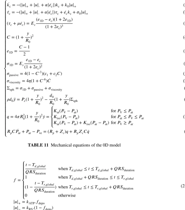
In this section we present results on the personalisation of 137 complete cases with a cardiac model. The cardiac model we use is a fast "0D" model which we introduced in18. It is a reduced version of our in-house 3D electromechanical model, based on the implementation of the Bestel-Clement-Sorine (BCS) model5 by Marchesseau et al.17,16 in SOFA2. As described in18, both the 3D and 0D model share the same mechanical and haemodynamic equations, but simplify-ing assumptions (see APPENDIX B) are made on the geometry of the 0D model. This leads to a very fast model made of 18 equations, which can simulate 15 beats per second at a heart rate of 75 bpm. In our context it is particularly practical for experiments which involve repeated personalisations of many cases, since the personalisation of a single case with CMA-ES as described in Section 2.4 takes around 3 minutes.
We consider a setP0Dof 6 parameters of the model, and a set of 4 measurementsO listed in Table 1 for which the 4
values are available for all the 137 cases.
The normalisation coefficients for this problem (in the vec-tor N defined in Section 2.4) are 10 ml for the Maximal Volume (MV) and the Stroke Volume (SV), 200 Pa for the Diastolic Aortic Pressure (DP) and the Mean Aortic Pressure (DP). With this normalisation, an error of fit√𝑆(𝑥, ̂𝑂) lower than 1 (resp 0.1), means a personalised simulation matches volume measurements within 10 ml (resp 1 ml) and pres-sure meapres-surements within 200 Pa (resp 20 Pa), which can qualitatively be considered as acceptable (very good).
3.1
Trade-off between Data-fit,
Regularisation and Dimension of the Set of
Personalised Parameters
We provide results of the IUP algorithm for at least 20 iter-ations, with both the Diagonal Matrix and the Full Matrix assumptions for values of 𝛾 of 0.5, 0.1, 0.05 (see names of the run in Table 2 ).
In Figure 3 , we report for each run the mean value
̄
𝑆(X, ̂O) of the data-fit term 𝑆(𝑥, ̂𝑂) and the mean value
̄
𝑅(X) of the regularization term 𝛾𝑅(𝑥) at convergence of
2www.sofa-framework.org
TABLE 1 Sets of 0D model parameters and outputs for which
the measurements are available in the example.
Personalised ParametersP Contractility 𝜎0
Resting Radius 𝑅0 Stiffness 𝑐1
Peripheral Resistance 𝑅𝑝 Windkessel Characteristic Time 𝜏 Venous Pressure 𝑃ve
OutputsO
Maximal Volume 𝑀 𝑉 Stroke Volume 𝑆𝑉
Mean Aortic Pressure 𝑀 𝑃 Diastolic Aortic Pressure 𝐷𝑃
Name 𝛾 Update FULL-IUP-005 0.05 Full Matrix FULL-IUP-01 0.1 FULL-IUP-05 0.5 DIAG-IUP-005 0.05 Diagonal Matrix DIAG-IUP-01 0.1 DIAG-IUP-05 0.5
TABLE 2 Names and parameters of the 6 runs of the IUP
algorithm
the MAP estimations (bottom). We also perform the Singular Value Decomposition (SVD) of the set of personalised param-eters and report the eigenvalues (Figure 3 , top). Then we report (rows of Table 3 ) the eigenvectors at the last iteration (𝑒𝑖, 𝑖= 1..6), and their corresponding eigenvalue (𝜆𝑖, 𝑖= 1..6). The eigenvectors coordinates are reported as 0 in bold when the value was below 0.01.
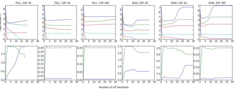
First we observe the classic phenomenon that the higher 𝛾 is, the higher the data-fit term (which characterizes the distance between simulated and measured values) is (Figure 3 , bottom, blue). A higher 𝛾 means that the noise (i.e. uncertainty on the measurements) is considered bigger in Equation 2 so estimated parameters values then tend to be closer to the prior mean than from a value which perfectly fits the measurements.
Second, that in every run of the algorithm, there is one or more eigenvalue which converges to 0 and is under10−4 at convergence. When the value is zero, this means that the parameters lie on a subspace of lower dimension. Here for each run, we report in Table 4 the number of eigenvectors with a eigenvalue above10−4, the mean value ̄𝑆(X, ̂O) of the
FIGURE 3 Top: value of the eigenvalues of the SVD of personalised parameters at each IUP iteration. Bottom: mean values
̄
𝑆(X, ̂O) and ̄𝑅(X) of the data-fit term 𝑆(𝑥, ̂𝑂) (blue) and the regularization term 𝛾𝑅(𝑥) (green) across the population at each IUP iteration. FULL-IUP-05 𝜎0 𝑅0 𝑐1 𝑃ve 𝑅𝑝 𝜏 𝜆𝑖 𝑒1 0.54 -0.31 -0.26 0.13 0.53 -0.50 3.62 𝑒2 -0.12 0.16 0.06 -0.74 -0.17 -0.62 2.73 𝑒3 -0.45 -0.69 -0.47 -0.25 0.03 0.15 1.34 𝑒4 -0.21 0.63 -0.66 -0.03 0.34 0.08 7.42e-5 𝑒5 -0.49 0 -0.05 0.61 -0.22 -0.58 5.42e-6 𝑒6 -0.45 0 0.51 -0.05 0.73 0 2.87e-9 FULL-IUP-01 𝜎0 𝑅0 𝑐1 𝑃ve 𝑅𝑝 𝜏 𝜆𝑖 𝑒1 0.38 0.09 -0.04 0.02 -0.55 0.74 4.80 𝑒2 0.68 -0.30 -0.41 0.33 0.42 -0.04 3.37 𝑒3 0.55 0.17 0.07 -0.64 -0.23 -0.45 2.31 𝑒4 0.08 0.69 -0.14 0.57 -0.25 -0.34 1.41 𝑒5 0.03 0.63 -0.06 -0.29 0.61 0.37 6.65e-5 𝑒6 0.30 0 0.90 0.27 0.19 0.02 3.13e-7 FULL-IUP-005 𝜎0 𝑅0 𝑐1 𝑃ve 𝑅𝑝 𝜏 𝜆𝑖 𝑒1 0.09 0.15 0.37 -0.68 -0.37 -0.49 5.03 𝑒2 0.46 0.11 -0.27 -0.06 -0.67 0.50 4.49 𝑒3 -0.72 0.29 0.38 0.11 -0.34 0.36 2.99 𝑒4 0.31 0.74 0.20 -0.14 0.47 0.27 1.12 𝑒5 0.14 -0.57 0.51 -0.31 0.21 0.50 5.73e-5 𝑒6 -0.39 0 -0.59 -0.64 0.20 0.23 1.10e-6 DIAG-IUP-05 𝜎0 𝑅0 𝑐1 𝑃ve 𝑅𝑝 𝜏 𝜆𝑖 𝑒1 0.16 -0.18 0 -0.35 0.90 0 3.91 𝑒2 -0.22 0.23 0 -0.91 -0.27 0 2.96 𝑒3 -0.92 0.20 0 0.20 0.28 0 1.88 𝑒4 -0.28 -0.93 0 -0.11 -0.18 0 1.11 𝑒5 0 0 1.00 0 0 0.04 2.08e-13 𝑒6 0 0 -0.04 0 0 1.00 3.71e-30 DIAG-IUP-01 𝜎0 𝑅0 𝑐1 𝑃ve 𝑅𝑝 𝜏 𝜆𝑖 𝑒1 0.12 -0.08 0 0 0.54 0.83 7.15 𝑒2 -0.46 -0.14 0 0 0.76 -0.44 4.44 𝑒3 0.86 -0.24 0 0 0.29 -0.33 3.04 𝑒4 -0.16 -0.96 0 0 -0.23 0.08 1.06 𝑒5 0 0 -0.31 -0.95 0 0 3.06e-13 𝑒6 0 0 -0.95 0.31 0 0 3.64e-17 DIAG-IUP-005 𝜎0 𝑅0 𝑐1 𝑃ve 𝑅𝑝 𝜏 𝜆𝑖 𝑒1 0.13 -0.08 0 0.02 0.50 0.85 7.06 𝑒2 0.51 0.13 0 0 -0.76 0.39 4.69 𝑒3 0.84 -0.24 0 -0.01 0.34 -0.35 3.18 𝑒4 0.16 0.96 0 0 0.23 -0.07 1.06 𝑒5 0 0 0 -1 0.01 0.01 0.17 𝑒6 0 0 -1.00 0 0 0 5.21e-14
TABLE 3 For each run of the IUP algorithm, final eigenvectors of the SVD of personalised parameters (𝑒𝑖) and their
corre-sponding eigenvalue 𝜆𝑖. In bold we emphasize the coordinates of eigenvectors which are lower than10−3and the eigenvalues
Run 𝛾 𝜆≥ 10−4 𝑆̄(X, ̂O) 𝑅̄(X) FULL-IUP-05 0.5 3 1.85 1.5 FULL-IUP-01 0.1 4 2.15e-2 0.40 FULL-IUP-005 0.05 4 6.18e-3 0.20 DIAG-IUP-05 0.5 4 0.65 2.04 DIAG-IUP-01 0.1 4 0.23 0.41 DIAG-IUP-005 0.05 5 1.96e-2 0.25
TABLE 4 For each run at the final iteration : number of
eigen-vectors for each run with a eigenvalue above 10−4 (column ’𝜆≥ 10−4’), mean data-fit value ̄𝑆(X, ̂O) across all cases and mean value ̄𝑅(X) of the regularization term.
data-fit term across all cases and the mean value ̄𝑅(X) of the regularization term.
From this table, we first observe that the mean of the
reg-ularization termis very close to 𝛾𝐷 where 𝐷 is the number of eigenvectors which do not have a value close to 0 (we use
𝜆 ≥ 10−4as the threshold for close to 0), which is consistent with Equation 10 of a cost function with a sparse regulariser on the dimensionality of the set of personalised parameters. We also observe that for the same 𝛾, the data-fit term is lower for the runs with the Full Matrix updates than the Diagonal
Matrix while having a lower number of non-zero eigenvalues.
More interestingly, we can observe the shape of the eigen-vectors at convergence of the algorithm. In every run with
Diagonal Matrix updates, we observe that the smaller the
eigenvalue associated to eigenvector is, the more it is aligned to a coordinate (a vector with shape (0,...,1,...0)). This means that for these runs, the parameters associated with these coor-dinates have a constant values in the final set of personalised parameters. In particular, the contractility 𝑐1 has always a constant value, and either 𝜏 (in DIAG-IUP-05) or 𝑃𝑣𝑒 (in DIAG-IUP-01) is constant as well. On the other hand, there is no such phenomenon in the runs with Full Matrix.
The behaviour of the algorithm can be understood from the sparse formulation explicited in 2.5 and the cost functions which is minimised. The algorithm indeed tries to find a prior for which there is an optimal trade-off between the number of dimensions of the set of personalised parameters, and the mean value ̄𝑆(X, ̂O) of the data-fit term. Given a specific 𝛾, the "cost" of lowering the dimension is an increase of 𝛾 in
̄
𝑆(X, ̂O). With the Diagonal Matrix updates, this is done with a constraint on the prior covariance matrix to be diago-nal so having a lower dimension means fixing the value of a parameter. On the other hand, with the Full Matrix updates, the algorithm can find any direction.
In particular we can observe than for 𝛾 = 0.1, both algo-rithms find a parameter subspace of dimension 4, but the data-fit ̄𝑆(X, ̂O) is higher with Diagonal Matrix updates
(0.23 ≥ 2.15e-2), where both 𝑐1 and 𝑃𝑣𝑒 are fixed. By
com-paring to the DIAG-IUP-005 where only the 𝑐1is fixed, we can interpret that the "cost" of fixing 𝑃𝑣𝑒 is a loss of around 0.23 on ̄𝑆(X, ̂O), which also means that the quality of some personalisations in the database is impacted.
Indeed, for the final personalisation of DIAG-IUP-01 there are at least 3 cases for which the personalisation is highly impacted (√𝑆 ≥ 3.5) because of the fixed value of 𝑃𝑣𝑒.
These cases have an aortic diastolic pressure which is par-ticularly low compared to the rest of the database 𝐷𝑃 ≤ 5400𝑃 𝑎. To fit this measurement, 𝑃𝑣𝑒 (which is the
asymp-totic and minimal value of the aortic pressure in the blood flow model) needs to be at least below this value (in particular in DIAG-IUP-005and FULL-IUP-01, all measurements of these cases are almost perfectly fitted and the estimated 𝑃𝑣𝑒for theses cases is≤ 5380𝑃 𝑎), but at this step the prior value of
𝑃𝑣𝑒in DIAG-IUP-01 (which is thus the fixed constant value) is5873𝑃 𝑎, which makes the fitting of the Diastolic Pressure impossible in these cases.
3.2
Parameter Existence and Uniqueness in
the Resulting Hyperplanes
A classical question in modeling and inverse problems, is to determine which parameters are observable with respect to a specific set of measurements. For example, here we estimate 6 parameters from 4 observed outputs. If there is a linear rela-tionship between the parameters and the outputs (i.e there exist a matrix M such asO(𝑥) = 𝑀𝑥), the size of the kernel of the matrix is at least 2. Considering some measurementsO, some parameters 𝑥 such as such asO = 𝑀𝑥, then for any vector y in the kernelO= 𝑀(𝑥 + 𝑦) as well. This means that there are at least two orthogonal parameter directions in which the param-eter values are unobservable. With a non linear-model (such as cardiac models), a similar phenomenon of non-uniqueness exists locally around some personalised parameters, to the extent that the model can be approximated by its gradient. In general, there is an entire manifold of parameters for which the outputs are the same.
Using Gaussian priors on such underconstrained linear mod-els leads a unique solution to the inverse problem, because in this case, the cost function 8 is strictly convex. To a cer-tain extent, this can be locally true for a non-linear model and a unique specific value is promoted within the manifold of parameters for which the outputs are the same.
Finding a (possibly unique) value which is the most
con-sistent considering a prior knowledge on the distribution of parameters is then the most interesting consideration of the MAP estimation, but this supposes to have an accurate prior. Since we are deriving the prior probability distribution from successive personalisations over the dataset itself, it is thus not
possible to rely on its interpretation as a "prior knowledge" to set parameter values in the unobservable directions of this
dataset.
On the other hand when no information on the statistics of the parameters is available, the only possibility is to perform a reduction of the parameter space, by forcing some parameter or parameter directions to have a fixed value. This can be done through PCA, PLS20or sensitivity analysis16on the parame-ters with respect to the clinical data, and estimate coordinates of the first modes only. This also leads to a few questions regarding the reduced space of parameters, particulary on the existence and uniqueness of parameter values for which the simulation fits the target data.
Here our parameters converge into a reduced subspace in all runs of the algorithm. In particular in the FULL-IUP-005, FULL-IUP-01, DIAG-IUP-005 run, there is also a very low data-fit term across the cases. This suggests that among the undetermined directions of a parameter space, with a small
enough prior, the algorithm selects an hyperplane of mini-mal dimension in which for each case, there is at least a set of parameter values which fits exactly the measurements.
We demonstrate this claim by analysing the resulting param-eter subspaces, in these terms of paramparam-eter existence and uniqueness. To that end we perform multiple personalisations without priors (i.e. an uniform prior, which is equivalent to solving Equation 8 without regulariser, or setting 𝛾 = 0) where parameter are taken from within these subspaces. Because the CMA-ES algorithm is stochastic, it usually converges toward different values of the parameters at each run if there are mul-tiple set of parameter values which minimise the cost function. We compare the following parameter subspaces:
1. The complete spaceH0of 6 parameters. 2. The subspace H𝑐
1 of 5 parameters of all parameters
except the stiffness 𝑐1, which is set to its final (constant) in the DIAG-IUP-005 run.
3. The 5 subspaces H(𝑐
1,𝜎0),H(𝑐1,𝑅0),H(𝑐1,𝑅𝑝),H(𝑐1,𝜏) and
H(𝑐1,𝑃ve) of 4 parameters where both the stiffness and
another parameter are set to the final prior mean value in the DIAG-IUP-005 run.
4. The 4 subspacesH5,H4,H3,H2of dimensions respec-tively 5,4,3 and 2, which are the hyperplanes defined by their center at the prior mean of the FULL-IUP-01, and the 𝑙 largest eigenvectors of the prior covariance for respectively l=5,4,3,2.
We then report both the mean error of fit √𝑆(X, ̂O) across all cases in the database, and the variability of esti-mated parameters across different personalisations, estiesti-mated by averaging across all cases the standard deviation of the 5 estimated values in the 5 personalisations.
TABLE 5 Mean error of fit and variability of personalised
parameters in 5 personalisations for the parameter subspaces. The value is reported as 0 if it is lower than10−3.
√ 𝑆 𝜎0 𝑅0 𝑐1 𝑃ve 𝑅𝑝 𝜏 H0 0 0.03 0 0.13 0.02 0.03 0.04 H𝑐1 0 0 0 - 0.02 0.02 0.03 H(𝑐1,𝜎0) 0.99 - 0 - 0.02 0.02 0.14 H(𝑐1,𝑅0) 3.90 0 - - 0.05 0.02 0.04 H(𝑐1,𝑃ve) 0.06 0 0 - - 0 0.06 H(𝑐1,𝑅𝑝) 0.07 0 0 - 0.07 - 0 H(𝑐1,𝜏) 0.01 0 0 - 0.02 0 -H5 0 0 0 0 0.015 0.017 0.03 H4 0 0 0 0 0 0 0 H3 1.99 0.03 0 0.002 0 0.004 0.01 H2 3.03 0 0 0 0 0 0
We first observe that the mean error of fit is 0 (lower than 10−3) for only four parameter spaces: the original spaceH
0, the parameter space H𝑐
1 with all the parameters except 𝑐1,
and the two parameter spaces H4 andH5 with respectively the 4 and 5 largest eigenvectors of the Full-IUP-01 run. This shows that they are the only subspaces which contain parameter values which fit the measurements for all cases.
Then among these subspaces, we observe that the only
subspace for which both the mean error of fit and the vari-ability of all parameters is 0 (lower than 10−3) isH
4, the hyperplane with the 4 largest eigenvectors of Full-IUP-01. In the other subspaces there is a variability from one personal-isation to the other for at least the haemodynamic parameters
𝑃ve, 𝑅𝑝and 𝜏 showing that the parameters are not unique. This shows that around the prior which was found in the DIAG-IUP-005run, 𝑐1was the only parameter which is pos-sible to set to a constant value without the personalisation of some cases being impacted (such as the 3 cases described in the previous section). However, once 𝑐1is set, the variability inH1 show that there is still an unobservable direction (especially in the haemodynamic parameters), but it is then necessarily a
combination of parameterswhich is unobservable.
Finally, because of the possibility to find subspaces which are not necessarily aligned with the coordinates, the Full-IUP-01 run was able to find a subspace of lower dimension, 4, in which there are parameters fitting all the cases and no variability, thus reducing the space in both directions of uncertainty.
3.3
Selection of a Parameter Subspace for
Personalisation
The resulting parameter subspaces in the previous section exhibit interesting properties in terms of existence and unique-ness of parameters for personalisation, so a question is how
relevant are they in the context of personalisation?First, it is important to observe that there is no guarantee of uniqueness of the parameter directions which are selected by the algorithm (and the personalised parameter either). Indeed, in addition of the model being non-linear (which makes the data-fit term not convex, thus the whole Equation 8), sparse regularisa-tions are usually not convex and have many possible soluregularisa-tions. In particular here, there are possibly multiple parameter sub-spaces on which the algorithm could converge. Visually, this can be observed in the schema of Figure 2 , where two differ-ent subspaces can be selected, each containing a unique set of parameter values for each of the 5 cases.
Secondly, there are no guarantees that the parameter spaces selected by the algorithm are relevant from a modeling or phys-iological point of view. In particular, when two parameters are not completely observable from some measurements in a database, their ’actual’ value (if they correspond to physical parameters) in a population is likely variable. In addition, a drawback of fixing a parameter to a specific value, is that it might force other estimated parameters to vary more within the population to account for variations which would have come from the fixed parameter.
Parameter selection in the sense of setting a specific parameter direction to a constant value is then an imper-fect approach in modeling, but it is unavoidable to not have variability in the estimation when no other information or statistics is available on this specific parameter direction.
In this context, though the selection of relevant parameters for personalisation cannot be performed entirely automatically (because the physical meaning of parameters is ignored by the algorithms), we believe that our algorithm can help the modeler by revealing unobservable parameter and parameter directions. To that end, we recommend the following gen-eral approach, considering a set of clinical data for which observable parameters are unclear:
1. First, perform one (or multiple) runs of IUP with
Diag-onal Matrix updates. This is because the resulting
sub-space is easier to analyze, since the parameters usually have a physical meaning in the context of modeling. Then analyze the parameters which end up with a eigen-value close to 0, and set them to a constant eigen-value if it is not incompatible with physiological considerations. 2. Second, perform one (or multiple) IUP with Full Matrix
updates to further select a lower dimensional subspace.
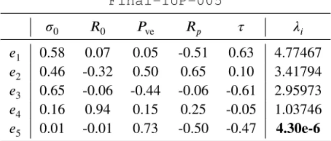
TABLE 6 Final eigenvectors and eigenvalues of the IUP run
with Full Matrix and 𝛾= 0.05 onH5. Final-IUP-005 𝜎0 𝑅0 𝑃ve 𝑅𝑝 𝜏 𝜆𝑖 𝑒1 0.58 0.07 0.05 -0.51 0.63 4.77467 𝑒2 0.46 -0.32 0.50 0.65 0.10 3.41794 𝑒3 0.65 -0.06 -0.44 -0.06 -0.61 2.95973 𝑒4 0.16 0.94 0.15 0.25 -0.05 1.03746 𝑒5 0.01 -0.01 0.73 -0.50 -0.47 4.30e-6
TABLE 7 Mean error of fit and variability of personalised
parameters in 5 personalisations inH∗. The value is reported as 0 if it is lower than10−3.
√
𝑆 𝜎0 𝑅0 𝑃ve 𝑅𝑝 𝜏
H∗ 0 0 0 0 0 0
We apply this approach to the current problem. First it seems physically likely that we do not have so much infor-mation on the stiffness 𝑐1 from only the 4 measurements in Table 1 , so we can reasonably decide to set its value to a constant, which we set at its value in DIAG-IUP-005. Then we perform a new run of the IUP algorithm, which we call Final-IUP-005, with Full Matrix and 𝛾 = 0.05 on the resulting parameters (thus in the hyperplaneH5). This leads to the final eigenvectors and eigenvalues:
We then select the hyperplane H∗ made of the 4 largest eigenvectors(𝑒1, 𝑒2, 𝑒3, 𝑒4) at the end of the run, and test the existence and uniqueness of personalised parameters in this hyperplane, with the same method than in the previous section. Results are reported in Table 7 .
As expected, both the variability of parameters and the mean error of fit are 0 (lower than10−3). This means that for each case, the hyperplane contains a unique (to the extent that we can evaluate it through this algorithm) set of parameter values for which the simulation fits the measurements.
To conclude, we found a minimal parameter subspace
of dimension 4, based on 5 parameters, consistent from a
physiological point of view, in which to perform consistent parameter estimation. More importantly, the final parameters
𝜇∗ andΔ∗ of the prior at the end of the Final-IUP-005 run respectively correspond to the mean and covariance of the estimated parameters, which we then call the population-based
priors.
Finally, we point out that the resulting population-based pri-ors will not necessarily correspond to the "real" underlying
parameter distribution. Indeed, considering a population with a known parameter distribution, the priors obtained through the IUP method will correspond to this distribution only if the data enables to completely determine the distribution parame-ters (in which case the influence of the prior will be minimal). However, if some parameters or parameter space directions are unobservable, the algorithm will choose arbitrary directions within the space, and build priors on these directions (which will result in dimensionality reduction to a minimal subspace). It is then up to the modeller to check that the selected subspace is relevant, possibly add additional output values to person-alised or, as we will see in the next section, enhance the dataset with other elements which can help determines the remaining unobservable directions.
4
CONSISTENT PARAMETER
ESTIMATION IN A DATABASE WITH
MISSING OR HETEROGENEOUS
MEASUREMENTS
In this section we present the application of the proposed framework to the consistent personalisation of a large
database of cases with heterogeneous (or missing) measure-ments. We present the personalisation of all the cases in such
database with the IUP* algorithm which leads to thefollowing properties of the personalised simulations:
1. All the measurements of all cases are well fitted in the corresponding personalised simulations.
2. Parameters lie on a reduced subspace of minimal and sufficient dimension.
3. Parameters for cases where measurements are missing are constrained by the population-based priors in this subspace which means in particular that unobservable parameters for these cases are guided by their values in the other cases of the database where they are available. In addition we also show in this section how the proposed framework can be extended to integrate external parameters such as the height and the weight of the patient in order to guide the estimation of parameters for cases where measurements are missing, leading to an improve consistency of parameter estimation for these cases.
4.1
Heterogeneous Database of Clinical Cases
We consider a larger database of 811 cases from different stud-ies, hospitals and protocols. Depending on the protocol, the same measurements are not available for all the patients and even within a single study with the same protocol, some mea-surements can be missing. To build this database, we focused
MeasurementsO Maximal Volume 𝑀 𝑎𝑥𝑉 Minimal Volume 𝑀 𝑖𝑛𝑉 Stroke Volume 𝑆𝑉 Ejection Fraction 𝐸𝐹 Mean Aortic Pressure 𝑀 𝑃 Diastolic Aortic Pressure 𝐷𝑃
TABLE 8 Measurements considered in the heterogeneous
database
on gathering patients and acquisitions for which the heart rate and at least one of the 6 following measurements in Table 8 was available:
Within this database of 811 cases, we have the following statistics:
• Pressure Measurements are available for 651 cases only.
• The Maximal Volume and Minimal Volume are both available for only 340 cases.
• Among the 471 other cases, either the Ejection Frac-tion (63 cases), Stroke Volume (386 cases) or no volume measurement at all (21 cases) are available.
• Ejection Fraction is the only measurement available in 38 cases.
• Stroke Volume is the only measurement available in 45 cases.
• 258 cases have a ’complete’ set of 4 measurements: Maximal Volume, Minimal Volume, Mean Aortic Pres-sure and Mean Diastolic PresPres-sure (we do not report Ejection Fraction and Stroke Volume if the Maximal Volume and Minimal Volume are already reported). In order to accommodate the heterogeneous nature of the database, we use a heterogeneous data-fit term. Instead of using the fixed formulation 𝑆(𝑥, ̂𝑂) =||(𝑂(𝑥) − ̂𝑂) ⊘N ||2 with 𝑂 being the vector of outputs(𝑀𝑎𝑥𝑉 , 𝑀𝑖𝑛𝑉 , 𝑀𝑃 , 𝐷𝑃 ) and ̂𝑂 the corresponding measurements, we build a differ-ent vector of observations for each patidiffer-ent. Depending on the available measurements, we use in the order of priority:
1. (𝑀𝑎𝑥𝑉 , 𝑀𝑖𝑛𝑉 , 𝑀𝑃 , 𝐷𝑃 ), 2. (𝑀𝑎𝑥𝑉 , 𝑆𝑉 , 𝑀𝑃 , 𝐷𝑃 ), 3. (𝑀𝑎𝑥𝑉 , 𝐸𝐹 , 𝑀𝑃 , 𝐷𝑃 ), 4. (𝑀𝑖𝑛𝑉 , 𝑀𝑃 , 𝐷𝑃 ), 5. (𝑆𝑉 , 𝑀𝑃 , 𝐷𝑃 ), 6. (𝐸𝐹 , 𝑀𝑃 , 𝐷𝑃 ), 7. (𝑀𝑎𝑥𝑉 , 𝑀𝑖𝑛𝑉 ), 8. (𝑀𝑎𝑥𝑉 , 𝑆𝑉 ), 9. (𝑀𝑎𝑥𝑉 , 𝐸𝐹 ), 10. (𝑀𝑖𝑛𝑉 ), 11. (𝑆𝑉 ), 12. (𝐸𝐹 ),
and a corresponding normalisation vector N . The normal-isation coefficient for the Ejection Fraction (EF) (which is a percentage) is 5%, it is 10 ml for the volume values (MaxV,MinV,SV) and 200Pa for the pressure values (MP, SP and DP).
As we explained in Section 3.1, the IUP algorithm with a constant noise as used in Section 3 realises a trade-off, driven by the constant 𝛾, between the number of dimension of the set of personalised parameters and the mean goodness of fit over the whole database. In particular by using a small 𝛾, a high goodness of fit was readched for all cases, leading to the selection of a minimal and sufficient subspace in where for each case of the database there is a set of parameter values for which the simulation fits exactly the measurements.
However on this heterogeneous database, selecting a small
𝛾 does not lead to a high goodness of fit for all cases. As we show in the next section (Section 4.2), an IUP run on the database of 811 patients with the heterogeneous data-fit term and 𝛾 = 0.05 (and even as small as 0.02) leads to a param-eter space of 3 directions instead of 4, and many complete
cases(with 4 measurements available) are not well fitted. This is because there are cases in the database with less than 4 measurements which can be well fitted with parameters in a parameter space of dimension 3 only. Consequently the con-tribution to the mean error of fit of badly fitted cases is small, which leads the algorithm to remove a parameter direction which is necessary to fit other cases. A possibility would be to use an even lower 𝛾, but this leads to practical numerical problems during the MAP estimation, because the value of the regularization term becomes too small in Equation 8 com-pared to the data-fit term. Instead, we use in the next section the IUP* version with reweighting of the data-fit term in the of the algorithm presented in Section 2.6.
4.2
Comparison between the IUP and IUP*
Algorithms on the Database
Here we demonstrate differences in the behaviour of the IUP
algorithm and the extended IUP* algorithm on this database.
We compare two runs of these algorithms, respectively called FULL-IUP-05and FULL-IUP*-05, based on the 5 param-eters ofH𝑐
1(the stiffness is set to a constant value), a value of
𝑔𝑎𝑚𝑚𝑎 = 0.05 and the Full Matrix updates. We first report as in Section 3.1 the number of eigenvectors with a eigenvalue above10−4at convergence, the mean data-fit value ̄𝑆(X, ̂O) across all cases and mean value ̄𝑅(X) of the regularization term, for each run in Table 9 .
We observe that the IUP run leads to 3 eigenvectors with an eigenvalue above10−4while the IUP* run leads to 4. The mean data-fit term value ̄𝑆(X, ̂O) for the IUP* run is very low (1.35e-3) and the IUP run is also low (1.01e-2). However we
Run 𝜆≥ 10−4 𝑆̄(X, ̂O) 𝑅̄(X)
FULL-IUP-05 3 1.01e-2 0.15
FULL-IUP*-05 4 1.35e-3 0.19
TABLE 9 For each run at convergence: Number of
eigen-vectors for each run with a eigenvalue above 10−4 (column ’𝜆≥ 10−4’), mean data-fit value ̄𝑆(X, ̂O) across all cases and mean value ̄𝑅(X) of the regularization term.
now show a boxplot which compares the repartition of the val-ues of the data-fit term error of fit√𝑆(𝑥𝑖, ̂𝑂𝑖) in the population in Figure 4 :
FIGURE 4 Comparison of the values of the error of fit
√
𝑆(𝑥𝑖, ̂𝑂𝑖) in the FULL-IUP-05 and FULL-IUP*-05
runs.
As we can see with the IUP run, there are many cases (almost one fifth of the population actually) which are not well personalised (√𝑆(𝑥, ̂𝑂)≥ 0.1). On the other hand in the IUP* run, by design of the algorithms all the cases have a data-fit term below 0.01.
Finally in Table 10 we also report, for the various possible values of the weight of the data-fit term 𝛼 (in Equation 11) at convergence, the percentage of cases in the population with these values. As we can see, this term doubled up to 4 times in some cases (thus leading to 𝛼= 16).
Overall, this section shows that the extended version IUP* enables a personalisation of the complete database where all
𝛼 1 2 4 8 16 % 81.79 0.49 1.47 9.85 6.4
TABLE 10 Percentage of cases in the population with the
cor-responding final value of 𝛼 in Equation 11 at convergence of the FULL-IUP*-05 run.
the individual cases have their measurements fitted within a specific value of the data-fit term, while parameters are
gathered on a parameter subspace of minimal and sufficient
dimension.
4.3
Parameter Estimation in cases of
Unobservability
Here we demonstrate the impact of the population-based pri-ors computed through the IUP* algorithm in this database on cases with unobservable parameters. To that end, we com-pare the estimated parameter values for cases where mea-surements are missing in two different parameter estimations for this database: first, the estimation of the 5 parameters
without priors and second, the estimation at convergence of the FULL-IUP*-05 run of the IUP* algorithm over the complete database and the 5 parameters.
The most interesting set of values is the following: in Figure 5 , we display the (log-)values of estimated parameters as a function of Ejection Fraction (resp Stroke Volume) for the cases where only the Ejection Fraction (resp Stroke Volume) is available. We observe a classic phenomenon with priors: per-sonalised values not only have less variance with the use of priors (blue points), but because one measurement has to be fitted, they also lie onto a space of (local) dimension 1. Indeed, this space is defined (in the case of the ejection fraction) by the equation
𝑥(𝐸𝐹 ) = 𝑎𝑟𝑔𝑚𝑖𝑛𝑥𝛾𝑅(𝑥) 𝑠.𝑡. 𝑆(𝑥, ̂O) = 0 (19) It is a space of local dimension 2 (resp 3) when 2 (resp 3) measurements have to be fitted (to the extent that the model is locally approximable to its gradient).
On an interpretative level, when some measurements are missing in our database and many parameter values are possi-ble, the personalisation with priors inH∗leads to the selection of a set of parameter values which maximises its likelihood in the probability distribution of the priors, or equivalently min-imizes the distance(𝑥𝑖− 𝜇∗)𝑇(Δ∗)−1(𝑥
𝑖− 𝜇∗). To that extent,
it performs a form of imputation in the parameter space by choosing the most likely set of parameters according to the distribution defined by 𝜇∗ andΔ∗. Since 𝜇∗ andΔ∗ are the statistics of the whole population of personalised parameter values, we argue that values of unobservable parameters and
parameter directions in some cases are then largely determined by their values in the other cases of the database where they are observable.
4.4
Integration of External Parameters in the
Prior Distribution for Improved Estimation of
Unobserved Parameters.
The key idea behind the use of priors is to model the distribu-tion of parameters in the populadistribu-tion. Then with the MAP esti-mation, the goal is to find the most likely parameters according to the correlations in this distribution. Here we explore the pos-sibility of integrating parameters which are not estimated into the prior distribution (we call them external parameters), to influence the value of estimated parameters.
Namely, for all our 811 cases, the height and weight of the patients were available. We can also consider the heart rate which is not an estimated parameter. In order to add these three parameters to the prior distribution, we perform the fol-lowing modifications to the method: in Equation 8, instead of considering a vector 𝑥 which only contains the parameters to be estimated, we use a concatenation vector of dimension 9 which contains the 6 estimated parameters and the 3 external
parameters. Formulations of the prior covariance and mean in Equations 2 and in the equations of Section 2.3 are adapted as well to accomodate this concatenation vector.
We then perform the following simple experiment: from the estimated parameters in Section 4.3, we estimate the covari-ance matrix and the mean of the concatenation vector, which we then use as a prior for a new estimation. This is equivalent to perform only one iteration of the IUP algorithm with Full
Matrix with this concatenation vector.
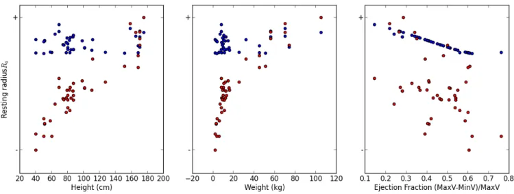
We report the most interesting result here in Figure 6 . For both the estimation without external parameters E1 (blue points) and with external parameters E2 (red points), we dis-play the estimated values of the resting radius 𝑅0for the cases where the Ejection Fraction is the only measurement, as a func-tion of a/ the height of the patient (left), b/ the weight of the patient (middle) and c/ the Ejection Fraction of the patient.
The results are the following: first in both estimations the goodness of fit for the cases in the database is similar and high (a mean error of fit of around 0.06). For the estimation without external parameters E1, the resting radius is well correlated to the Ejection Fraction (this was already observed in Figure 5 ), but not at all to the weight and the height. However with the external parameters E2, the values of the resting radius is very
correlated to the height and weight of the patients, and tends
to increase with both these measurements. Since the resting radius, from a physical point of view, is related to the size of the heart, this correlation makes sense from a physical point
FIGURE 5 Top: (resp Bottom:) Log-value of estimated parameters value as a function of the Ejection Fraction (resp Stroke
volume) for the 38 (resp 45) cases where only the Ejection Fraction (resp Stroke Volume) is available, in blue with the IUP*
algorithm, in red without priors.
FIGURE 6 Estimated values of the resting radius 𝑅0 in the estimation without external parameters (blue points) and with
external parameters(red points) in the prior distribution, for cases where only the Ejection Fraction was available (the resting radius was thus not completely observable).
of view and leads to an improved consistency of the estimated values in E2 than in E1.
5
CONCLUSION
In this manuscript we introduced a method called Iteratively
Updated Priors which performs successive personalisations
of the cases in a population, where the prior probabilities on parameter values at each iteration are set from the statistics