COMPUTER SIMULATED VISUAL AND TACTILE FEEDBACK
AS AN AID TO
MANIPULATOR AND VEHICLE CONTROL
by
Calvin McCoy W.ney III
S.B. MASSACHUSETTS INSTITUTE OF TECHNOLOGY
SUBMITTED IN PARTIAL FULFILMENT OF THE REQUIREMENTS FOR THE
DEGREE OF MASTER OF SCIENCE IN MECHANICAL ENGINEERING
at the
MASSACHUSETTS INSTITUTE OF TECHNOLOGY June 1981
Massachusetts Institute of Technology 1981
Signature of Author
Certified by
Department of Mechlnical Engineering
May 8,1981 C Thomas B. Sheridan Thesis Supervisor Accepted by
Archives
MASSACHUSETTS INSTITUTE OF TECHNOLOGYJUL
3 1 1981
Warren M. Rohsenow Chairman, Department Committee---COMPUTER SIMULATED VISUAL AND TACTILE FEEDBACK
AS AN AID TO
MANIPULATOR AND VEHICLE CONTROL
by
CALVIN McCOY WINEY III
Submitted to the Department of Mechanical Engineering on May 8, 1981 in partial fulfilment of the
requirements for the Degree of Master of Science in Mechanical Engineering
ABSTRACT
A computer graphic simulation of a seven
degree-of-freedom slave manipulator controlled by an actual master was
developed. An electronically coupled E-2 manipulator had
previously been interfaced to a PDP-11/34 by K. Tani, allow-ing the computer to sense and control each degree of freedom
independently. The simulated manipulator was capable of
moving an arbitrarly shaped object and sensing a force in
an arbitrary direction with no actual object or force
exist-ing. The simulated manipulator could also be attached to a
simulated vehicle capable of motion with six
degrees-of-freedom. The vehicle simulation is currently being used in
conjunction with dynamic simulations developed by H.
Kazer-ooni to test different types of dynamic controllers for
submarines. Shadows, multiple views and proximity indicators
were evaluated to determine their effectiveness in giving
depth information. The results indicated that these aids are
useful. Subjects felt that shadows gave the best perception
of the environment, but found isometric views easiest to use
on the tasks performed. This type of simulation appears to
be realistic and adaptable to a multitude of applications. Thesis Supervisor: Thomas Sheridan
Title: Professor of Engineering and Applied Psychology
ACKNOWLEDGEMENTS
I wish to thank Professor Thomas Sheridan for his
many words of advice and encouragement. I appreciate the op-portunity to work in the Man-Machine Systems Laboratory, it has been a most interesting and educational experience.
I would like to thank my many friends at the
Man-Machine Systems Lab for making it an enjoyable place to work. Special thanks must go to my friend and co-reseacher, Homa-yoon Kazerooni, who developed the vehicle dynamics simula-tion and helped me interface it with the graphic simulasimula-tion. I would also like to thank Don Fyler for his suggestions on
improving the simulation, Dana Yoeger for helping me to
understand the computer system and Ahmet Buharali for
help-ing to maintain the computer. A word of thanks must go to
all the people who put time into performing my experiments
at a very busy time in the semester.
Finally, I wish to thank my fiancee, Deborah Darago,
for her help on the statistical analysis of the experments,
for proofreading this document and for her patience and
understanding during the many hours spent working on this
project.
This work was supported by the Office of Naval Research, Contract N00014-17-C-0256, monitored by Mr. G Malecki, Engineering Psychology Programs.
TABLE OF CONTENTS
ABSTRACT ... ... 2
ACKNOWLEDGEMENTS ... LIST OF FIGURES AND TABLES ... ... 6
INTRODUCTION AND PROBLEM STATEMENT...8
Artificial Intellegence Versus Supervisory Control... 8
Computer Generation of Operator Feedback...9
Simulation of Master-Slave Manipulators...10
Depth Perception From Two-dimensional Images...11
APPLICATIONS OF COMPUTER GRAPHIC MANIPULATOR SIMULATIONS..13
Simulation of Various Operating Conditions...13
Testing of Control Systems...13
Supplementation of Operator Feedback...14
Rehearsal... ... 15
Humanizing Man-Computer Interactions...16
DISPLAY THEORY AND DEVELOPMENT...17
Data Storage ... ... ... ... 17
Translations and Rotations... e... ... ... ... 19
Shadow Generation...c....e e....24
Moments of Inertia.... ... . ... 26
Body and Global Coordinates...27
Generation of Force Feedback... ... 28
Resolved Motion Rate Control. ... 34
Control of the Manipulator... 35
Touching Cc EQUIPMENT... PDP11/34 C E-2 Master Megatek Di EXPERIMENTAL Programmin Manipulato Depth Indi Experiment RESULTS AND Master-Sla Simulated Depth Indi Conclusion REFERENCES.. APPENDICES.. I Depth In II Simulat III Force-IV Auxilla V Manipula VI Submari VII Manipu VIII Progr onditions ... 38 omputer ... 43 -Slave Manipulator...45 splay Processor... ... . 45 DESIGN ... 47 g Considerations... ....47
r and Vehicle Simulation... 50
cators ... 53
al Measurement of Operator Performance...54
CONCLUSIONS.. ... ..... ... 55
ve Simulation ... 55
Force-Feedback... ... . . ... . .. . 64
cators.•... •... 66
s and Recommendations ... .. 70
dicator Experiment Statistics...73
ion Transformation Matrices ... 80
Feedback Jacobian Calculation...86
ry Software ... .... . ... 88
tor Simulation Software... 90
ne Simulation Software...107
lator Control Software...126
LIST OF FIGURES AND TABLES
Figure 1 Manipulator and Vehicle Angles...18
Effects of Order of Rotation... Equivalent Body and Global Rotations.. Master-Slave Manipulator Block Diagram Computer Controlled Master Block Diagr Multiple Spherical Touching Conditions Multiple Spherical Touching Conditions Rectangular Touching Conditions... Man-Machine Systems Laboratory... E-2 Slave Manipulator... Figure Figure Figure Figure Figure Figure Figure Figure Figure Figure Figure Figure 2 3 4 5 6 7 8 9 10 11 12 13 Display Type 2 - Front and Sid Display Type 3 - Front View wi Indicator... ... 22 ... 29 ... 30 am. ... 30
... 40
... 40
... 42
... 44
... 46
Walls... ... 56 e Isometrics. th Proximity Display Type 4 - Proximity Indicator Manipulator Simulation with Shadows. Manipulator Simulation with Shadows. Detail of Tongs Gripping a Rectangul Simulated Surface... Deflection of Simulated Surface ... Deflection of a Soft Surface... Deflection of a Hard Surface... Submarine Simulation... Evaluation of Depth Indicators... .... 56 Alone.... .57 ... 59 ... 60 ar Peg ... 61 ... 62 ... 62 ... 63 ... 63 ... 65 ... 68 Display Type Figure Figure Figure Figure Figure Figure Figure Figure Figure Figure - Shadow with 14 15 16 17 18 19 20 21 22 23 ... 57Table 1 Table 2 Figure 24 Figure 25 Figure 26 Figure 27 Table 3 Table 4 Table 5 Table 6 Table 7 Average Time to Average Time to Learning Curves Learning Curves Learning Curves Learning Curves Average Time to Average Time to Average Time to Locate Object Locate Object - Subject I... - Subject 2... - Subject 3... - Subject 4... Locate Object Loacte Object Locate Object Three-Way Analysis of
Control Interface I/O
Variance Channels - Subject I ... - Subject 2.... - Subject 3.... - Subject 4.... - All Subjects. ... ..73 .. 73 .. 74 .. 75 ..76 .. 77 ..78 6.78 .. 78 .. 79 .126
INTRODUCTION
In the past several years, develpoments in the elec-tronics industry have made mini-computers extremely small, powerful and inexpensive. Microprocessors are now being in-corporated in machinery ranging from large scale production equipment to household dishwashers. As this trend continues, more effort will be put into the use of the computer to aid the human operator. Automobiles are already on the market which use microprocessors to control automobile function and relay failure information to the driver. As computers become more common, the question will arise as to how they can best serve the operator.
Artificial Intelligence Versus Supervisory Control The use of computers to aid human operators can be divided into two catagories: artificial intelligence and supervisory control. The major difference between the two approaches is in the manner in which the computer interacts with the human operator. Artificial intelligence ( A. I. )
attempts to give the computer maximum intelligence and to replace all operator functions by the computer. Supervisory control acknowledges that the operator has certain abilities. It attempts to use those talents and supplement those which are lacking.
The task of removing a bolt from an undersea struc-ture emphasizes the differences between these two approaches.
The A. I. approach might require the computer to
differen-tiate between the pilings and the surroundings, to be able
tell a bolt from a barnacle and be able to select the proper
bolt. It must also be able to determine the proper angle at
which to turn the nut, be able to select the proper tool to
fit that nut and cope with the possability of the nut being
damaged. The supervisory control approach would rely on the
operator to find the bolt, while possibly aiding with image
enhancement. The operator would determine the proper tools
and condition of the bolt. If the vehicle were moving, the
computer might aid the operator by compensating for that
mo-tion. The computer would then remove the bolt after the
operator showed it the proper orientation and described the
desired motion.
The A. I. approach becomes necessary when
circum-stances make operator interaction impossable. Its major
drawback is that it requires extensive programming in
order to cope with all possible contingencies. The more
variable the environment; the more complex the required
pro-gramming becomes. The supervisory approach achieves economy
by taking advantage of the operator's abilities ( experience
and intuitive skills ) while the computer supplies memory,
accurate position control, speed and repeatability. Computer Generation of Operator Feedback
inter-action, one important way in which a computer can aid an operator is to improve the operator's knowledge of his en-vironment. Feedback can take many forms, though humans rely most heavily on their tactile, visual and auditory senses. Improved feedback is important for several reasons. Supply-ing the operator with more processed information leaves the operator more time to dedicate to the task. Any information can be related to the operator by a set of numbers, however the some types of feedback are more easily assimulated than others. The orientation of a vehicle can be completely described by a set of angles, however a display of the vehicle is more informative even though it is less accurate. Feedback may exist, but it may be of poor quality. In this case, the computer could be used to improve rather than create feedback.
Several forms of feedback can be used simultaniously to reinforce the operator's perception of the environment. For example, combining tactile with visual feedback may be a better aid than either tactile or visual feedback alone. A single type of feedback may not be best suited for all tasks. The use of several different types of feedback could allow the operator to select the type of feedback he preferred for each type of task.
Simulation of Master-Slave Manipulators
of a computer graphic simulation of a master-slave manipu-lator. The simulation was controlled by an E-2 master mani-pulator which had previously been interfaced to a PDP11/34 computer by K. Tani (7). This interface allowed the computer to sense and control each of the seven degrees of freedom of the manipulator independently. Part of the simulation in-cluded the development of an environment within the computer which the simulated manipulator could interact with. The si-mulated manipulator was capable of moving an arbitrarly
shaped object about in three-dimensional space and simulat-ing force-feedback in an arbitrary direction. Force was felt when the manipulator grasped an object or touched a prede-fined surface. The simulated manipulator could also be at-tached to a vehicle capable of motion with six degrees-of-freedom. The vehicle simulation is currently being used by H. Kazerooni to test various types of dynamic controllers
for small underwater vehicles.
Depth Perception From Two-Dimensional Images
One of the difficulties common to both generating graphics of a three-dimensional system and to performing manipulation via closed-circuit television is the lack of ability to perceive three dimensions. The method of display-ing depth would appear to be particularly critical in appli-cations such as manipulation which require physical motion
object from a moving vehicle require the ability to quickly integrate the two-dimensional image plus the depth cues into three-dimensional motion. If the information cannot be as-similate quickly, the object will have moved relative to the operator by the time its position has been determined. A close spatial relationship between the display and the real world would appear to make interpreting the display easier.
Shadows, multiple views and proximity indicators were tested to determine their effectiveness as depth cues. Each depth indicator was chosen for exemplifying a partic-ular attribute. The shadow was chosen because it is the most familiar depth cue and has a strong spatial relationship. Its drawbacks are that it compresses picture information and the e is the possablity that several shadows near one an-other may make interpretation difficult. The front and side isometric projections normally used in mechanical drawings give depth information more clearly than the shadow, but determination of depth from the side view may cause some coordination problems. Both of these depth indicators re-quire extensive prior knowledge of the environment. The proximity indicator which measures the distance between the manipulator tongs and the desired destination could be dis-played with little prior knowledge of the environment. In practice, proximity could be determined by a sonar mounted on the tongs. The proximity indicator was displayed along
with a front view of the manipulator. The proximity indi-cator, with no other display, was used as a control.
APPLICATIONS OF COMPUTER GRAPHIC MANIPULATOR SIMULATIONS Simulation of Various Operating Conditions
A realistic simulation can be of value both for
ex-permentation and for operator training by simulating
envi-ronments which can not be easily created in a laboratory.
The viscosity and the change in the relationship between
weight and mass associated with underwater work can be
simu-lated without requiring tanks of water or undersea
manipu-lators. The zero-gravity conditions associated work in space
such as the space shuttle can be easily simulated by a
com-puter, but would be very difficult to obtain in a laboratory by any other means.
By using a computer to control a manipulator, it is
possable to vary the properties of that manipulator so that
it can be used to simulate many types of manipulators.
Mo-ments of inertia can be changed to make a light hot-room
manipulator behave like a massive industrial manipulator.
Several degrees-of-freedom of a seven degree-of-freedom
manipulator can be locked to simulate a less flexible
manipulator.
Testing of Control Systems
Building a control system for a vehicle can be an
need to be modified and sensors need to be installed. With a new controllor there is always the risk of instablity and failure which could result in damaged hardware. When creat-ing a control system for a one-of-kind vehicle, the money and time lost in a failure could make improvement or addi-tion of a control system prohibitive. Using a computer simu-lation would allow the prototype controllor to be changed quickly and easily. Propulsion and sensor configurations could be tested without the need for expensive hardware. Failure of a computer simulation generally involves essen-tially no risk. Therefore, a simulation can be run during an instability to collect additional data on the failure with out the risk of hardware damage.
Supplemention of Operator Feedback
Due to the high cost of using humans directly, un-manned submersibles are used to inspect and repair offshore
oil rigs in the North Sea. To avoid tethering problems, com-municatons to the operator on the surface can be via
accous-tic link. One difficulty with an accoustic link is that it is only capable of low bit rate transmission. The bit rate is the product of the frame rate, number of bits of gray scale and the number of pixels ( resolution ). A 200 by 200 pixel picture with 5 bits of grey and a frame rate at the flicker limit of 15 frames per second requires transmitting 3 million bits per second. To the operator who is watching
the work via a television picture sent through an accoustic link, this means he receives a very degraded picture (3). Since the manipulator position can be completely defined by knowing each angle of the seven degrees-of-freedom to 16 bits, these 118 bits can be transmitted freqently allowing the simulation to be updated frequently. By superimposing a rapidly updated simulation of the manipulator on a slowly updated but high resolution television picture, data trans-mission can be optimized such that the moving portion of
the display is refreshed frequently while the static visual background is of good quality.
In the case of poor visability, a simulation could be used to generate or enhance the view of the surroundings. If part of the environment was known in advance and stored in the computer, it could be displayed on the simulation as soon as the operator established enough reference points to locate and orient the environment relative to the operator. Objects could also be inputted into the display by feeling about and recording points of contact. The points of contact could then be analyzed to determine the location of surfaces and edges.
Rehearsal
When an operator is required perform a dangerous or delicate task where a mistake might harm the operator, the
equipment or the task, it might be desirable for the
-15-ator to be able to practice the task first before actually
performing it. If a realistic simulation was available, the
operator could practice the task on the simulation until he
felt confident to actually execute the task. If the
manipu-lator were computer controlled, the operator could perform
the task on the simulation until he performed the task
per-fectly. The computer could moniter each practice run. When
the operator was satisfied with a run, he could tell the
computer execute that run. The computer would then duplicate the previous motion (6).
Humanizing Man-Computer Interaction
It has been suggested that a standard master
manipu-lator or a smaller table-top version be used as a means of
communicating with a computer. The manipulator used in these
experiments had seven degrees-of-freedom which allowed the
tongs to be moved to any position and orientation within
range. It was also capable of force-feedback which allowed
it to communicate contact with an object to the operator.
One of the difficulties with CAD systems is developing the
ability to input three-dimensional data. A manipulator could be used as a three dimensional digitizer. The spatial
qual-ity of the manipulator might help in inputting points which
were three-dimensional in nature. The manipulator could send
force-feedback when the operator touched a point or line in
desired points were all on a given plane, computer control
could be used to restrict movement to that plane. When the
desired object had been inputted, it could be easily
exam-ined by grasping it and rotating it as if it were in one's
hand.
The manipulator could also be used in a more
ab-stract way. Data could be encoded with spatial, tactile or
physical properties. A particular point might be hard or
soft, heavy or light, or sticky or slippery. This might be
helpful in aiding the operator to select a particular type
of data while searching through a data space. It might also
help him to notice small differences between attributes. If
he were looking for a particular type of data, the computer
could use force-feedback to "push" him in the right
direc-tion (6).
DISPLAY THEORY Data Storage
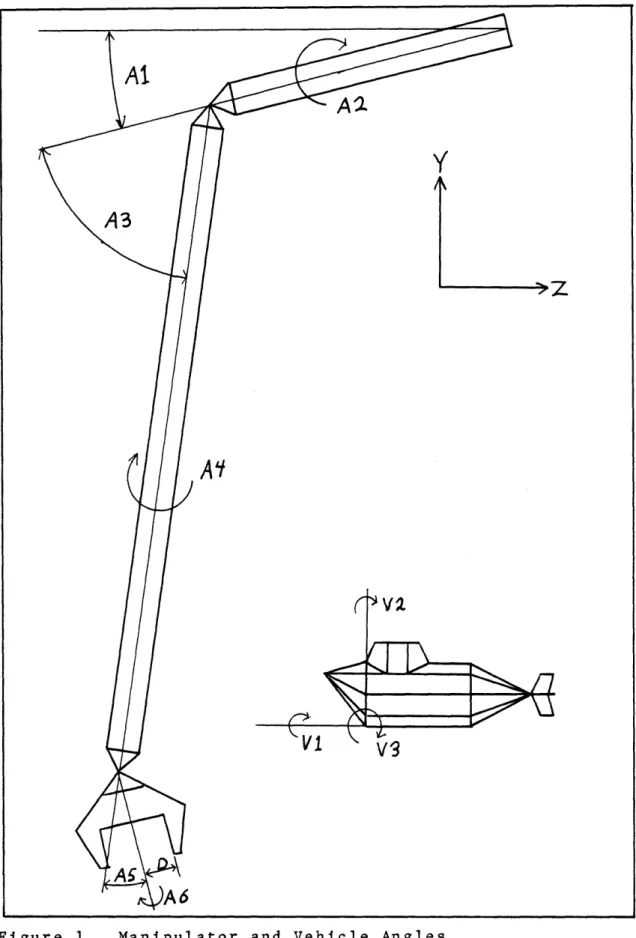
A schematic of the manipulator and vehicle with
the definitions of the degrees-of-freedom is shown in figure 1. The arm, submarine and object were stored in stan-dard point-connectivity data form. The arm was broken into
three distinct portions, the shoulder, forearm and tongs.
Each section of display was treated as a separate entity.
The data base for each section was stored in an unrotated
reference frame with the center of rotation located at the
-17-A~
VVl
'3
Figure 1 Manipulator and Vehicle Angles
f
origin. The vehicle was stored so that forward motion of the unrotated vehicle was in the negative z direction. Each sec-tion of the arm extended from the origin along the negative z-axis. This reference frame was the same as that of the display terminal. In this right-handed coordinate system, the x-axis was to the right, the y-axis was upwards and the z-axis was out of the screen. The origin was at the center of the screen. Each element had a corresponding rotation matrix containing the transformations required to move the element from the reference frame to its desired location. Objects which could be manipulated also had a set of touch-ing conditions which were defined in the reference frame.
Translations and Rotations
The multiple rotations required to display the arm were most easily calculated in matrix form. The matrix ele-ments were fed directly into the display processor's hard-ware matrix multiplier. All rotations were based on global coordinates. A translation Tx in the X direction is given by:
X' = X + Tx
In three dimensions this can be expressed in matrix form as:
1
1
0 0
Tx
X
OY' - 0 1 0 Ty Y Z' - 0 0 1 Tz Z1
0 0 0 1
1
-19-where the ones in the coordinate matrices satisfy the matrix algebra needed to add the constant Tn. This matrix form can
be abbreviated as:
X' = TX
T is called the translation matrix. Transformation matrices can also be formed for rotations in the same manner. The ro-tation matrix Rx for a roro-tation of an angle A about the x-axis is:
Rx 1 0 0 0
0 cosA -sinA 0 0 sinA cosA 0
0
0
0
1
Rotation matrices about the y and z-axis are given by:
Ry cosA 0 sinA 0 Rz- cosA -sinA 0 0
0
1
0
0
sinA cosA
O 0
-sinA 0 cosA
00
0
1
0
0 0 0 1 0 0 0 1
These rotation matrixes are for rotation about the origin. To rotate about an arbitrary point, one must translate the desired center of rotation to the origin, perform the ro-tation, then translate the center of rotation back to its original position (4,5).
A series of transformations can be reduced to a sin-gle transformation matrix by matrix multiplication. Since matrix multiplication is associative but is not
commuta-tive, the order in which transformatioms are performed is
important. Rotation about the x-axis and then about the
z-axis is not the same as rotation about the z-axis and then
about the x-axis. This is most easily seen by the example
illustrated in figure 2. If one holds one's right arm out to the side with the palm facing downward and a coordinate
sys-tem is established so that the y-axis is upward and the
x-axis extends to the right parallel to ones arm, then the
z-axis extends out behind. If the forearm is rotated 90
degrees about the x-axis, then 90 degrees about the y-axis,
the forearm is pointed forward and the palm is facing to the
left. If the forearm is first rotated 90 degrees about the
y-axis, then 90 degrees about the x-axis, the forearm is
facing upward and the palm is facing foreward.
Transfor-mation matrices occur before the coordinate matrices and are
sequenced in the order in which they occur from right to
left as follows:
X' A
'XI
An
...
A3
A2 Al X
In this simulation it was necessary to be able to
perform the reverse coordinate transformation. This requires taking the inverse of the transformation matrix. The inverse of A is found by:
A-l=adj(transpose(A)
)/det()
Figure 2 Effects of Order of Rotation
n
-determinants of 16 3x3 matrices, each of which requires 5
additions and 6 multiplications, for a total of 176
opera-tions. Since the bottom row of the transformation matrix is
only used to satisfy the matrix algebra and contains no
in-formation, the transformation matrix can be partitioned into a 3x3 rotation matrix and a 1x3 translation matrix:
The coordinate transformation is then given by:
X' =RX+T
This can be solved for X to give:
Computing the adjoint of a 3x3 matrix requires finding the
determinants of 9 2x2 matrices, each of which require 1 add-ition and 2 multiplications for a total of only 27 opera-tions. The new transformation matrix can be reconstructed by rejoining the new rotation and translation matrices as:
1110
R T1
For the general rotation matrix, R
XX XY XZ XT
YX YY YZ YT ZX ZY ZZ ZT
0
0
0
1
the components of the inverse matrix,
RXX RXY RXZ RXT RYX RYY RYZ RYT
RZX RZY RZZ RZT
0
0
0
1
are fould to be:
RXX-(YYZZ-ZYYZ)/Det RXZ=(XYYZ-YYXZ)/Det RYX-(YZZX-YXZZ)/Det RYZ- (YXXZ-YZXX)/Det RZX-(YXZY-YYZX)/Det RZZ-(XXYY-XYYX)/Det where det is the determinant given by: RXY= (ZYXZ-XYZZ)/Det RXT -RXXXT-RXYYT-RXZZT RYY=(XXZZ-XZZX)/Det RYT -RYXXT-RYYYT-RYZZT RZY=(XYZX-ZYXX)/Det RZT=-RZXXT-RZYYT-RZZZT
of the rotation matrix and is
De t=XXYYZZ+XYYZZX+XZYXZY-ZXYYXZ-ZYYZXX-ZZYXXY
The determinate of a rotation matrix is formally one,
how-ever it was calculated to compensate for roundoff error by
the computer.
Shadow Generation
If the source of illumination is far enough from an
object that rays passing through different points can be
considered parallel, then its shadow can be represented by
matrix notation. If the source of illumination is directly
the y-coordinate of every point in the shadow is at the height of the surface Ys and x and z values remain unchanged. The transformation matrix for this shadow is:
1 0 0 0
0
0 0 Ys
0 0 1 0
0 0 0 1
If the surface can be expressed as a linear function of x and z as given by:
y=Ax+Bz+C
then the transformation matrix for a shadow cast on this surface is given by:
1 0 0 0
A 0 B C 0 0 1 0
0 0 0 1
It is also possable to accomodate light coming in from an arbitrary angle. Suppose the light is from an angle (a) from the y-axis, as measured about the z-axis and the surface is horizantal at Ys. The x component of the shadow remains the same as that of the object, the y component is at the sur-face value Ys. The z value is determined from the distance between the surface and the object and the angle of illumi-nation.
X'=X Y'=Ys
Z'=Z-(Y-Ys)Tan(a)
-25-The transformation matrix is then:
1
0
0 0
0 0 0 Ys
0 -Tan(a)
1 YsTan(a)
0 0 0 1
Shadows on different surfaces and illumination from differ-ent directions can be handled in a similar manner.
Inertia
It is hoped future vehicle simulations will include manipulator-vehicle interactions such as those which occur when manipulating a massive object from a small, light ve-hicle. This will require determining the moment of inertia of the manipulator for any position. If the centroidal mo-ment of inertia Ic is known for each unrotated section of the manipulator, then the moment of inertia for any manipu-lator configuration can be determined (2). First the iner-tance must be calculated for the proper orientation of each segment of the manipulator. If a segment is described by a rotation matrix R, were R is the rotation portion of the transformation matrix, then the inertance Ir for the rotated segment is given by:
YIrRIc
=
The final moment of inertia I' about the shoulder can the be found by applying the parallel axis theorem. If Xt, Yt and Zt are the distances from the shoulder to the centroid
of the segment in question and M is the mass of the section, then the inertance is:
I'=RIcRrT +M -XtYt Xt2+Zt2 -YtZt
-XtZt -YtZt Xt2+Yt2
If Xc is the vector describing the location of the centroid
in the unrotated reference frame, then the vector Xt is
found to be:
Xt=RXc
Since the manipulator is oriented along the z-axis, if the
manipulator is relatively symmetric about the z-axis, Xc and Yc are zero, in which case the elements of Xt are simply:
Xt-XZXc+XT Yt=YZYc+YT
Zt-ZZZc+ZT
Global and Body Coordinates
The orientation of a vehicle is normally expressed in the body-referenced Euler angles yaw, pitch and roll. The order of rotation is yaw, followed by pitch and finally roll. The reason for this convention is that forces on a body are
generally invarient with respect to changes in orientation
when they are described by body coordinates. The dynamic programs developed by H. Kazerooni are based on body center-ed coordinates. Since the display processor is based on
global coordinates, a method of transforming from body
Examination of motions of the vehicle reveals that the rotations yaw, pitch and roll in body coordinates are the same as roll, followed by pitch and then yaw in global coordinates. Before any rotation, global and body coordi-nates are equivalant ( Figure 3 ). Roll about global and body axis is therefore the same. After this rotation, pitch about global coordinates performs the same function as it did in body coordinates. Final yaw performed in global coor-dinates after these transformations is still the the same as yaw performed first in body coordinates.
Generation of Force-Feedback
In normal manipulator operation, the only informa-tion transfer between our master and slave manipulator is positional information. The control interface allows
posi-tional information to be transferred between computer and manipulator. Since there is no means of directly sending force information to the manipulator, generation of force-feedback involves encoding force information into a posi-tional signal.
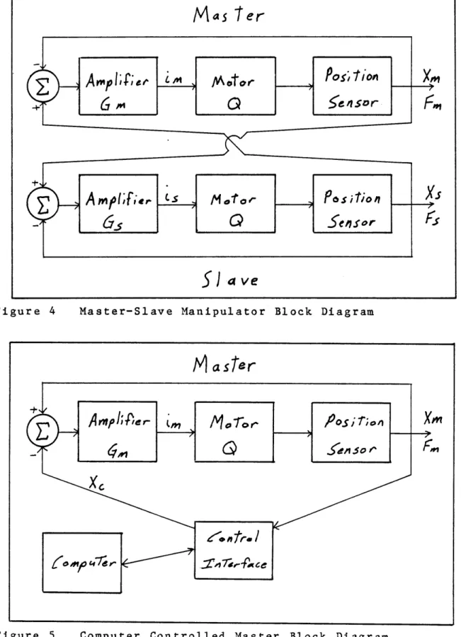
To understand computer generated force-feedback, one should first understand the operation of the manipulator in master-slave mode. Figure 4 shows the configuration of the manipulator in this mode. Each manipulator is made up of a set of servomotors, each of which is directly coupled to a potentiometer. Each servomotor is driven by an amplifier
~i)
L~-x
a
4
4,
A -AL IK
Roll
1
P
;
re
h
1~
Y&/
Figure 3 Equivalent Body and Global
x I Rotations -29-I I ww nI
I
f"-x
nui r10
·XFigure 4 Master-Slave Manipulator Block Diagram
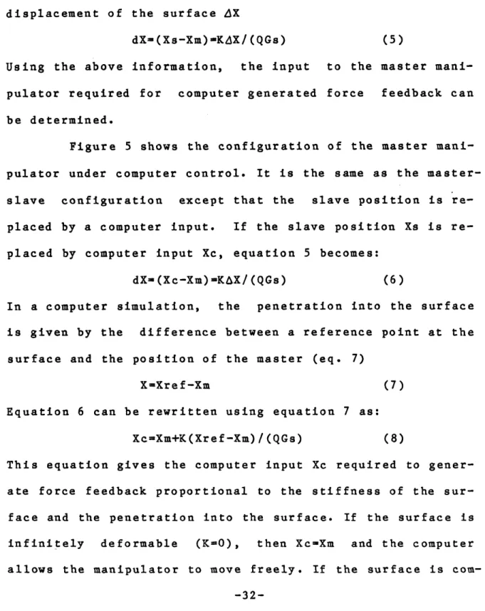
Figure 5 Computer Controlled Master Block Diagram
Mas ter
5 ave
M
aster
that outputs a current which is proportional to the differ-ence between the master and slave positions. If Xm and Xs are the master and slave positions respectively, and Gm and Gs are the gains of the amplifiers associated with the mas-ter and slave, then the currents input to the servomotors are given by:
is=Gs(.Xm-Xs)
im=Gm(Xs-Xm)If Q represents the gain of the servomotors in converting current into force, then:
Fs-QGs(Xm-Xs) (1)
Fm=QGm(Xs-Xm) (2)
Combining equations 1 and 2 yeilds:
Fs=-FmGs/Gm (3)
or force on the master is directly proportional to the force on the slave.
Since only positional information is transferred between the master and slave, how that information relates
to forces on master and slave needs to be considered. If the slave is pressing on a linear elastic surface, the force on the slave is given by:
Fs=KAX (4)
which is the conventional spring law where AX is the dis-placement of the surface and K is the spring constant. Com-bining equations 3 and 4 gives the resulting force felt through the master:
-31-Fm--KAXGm/Gs
Combining equations 1 and 4 and solving for (Xs-Xm) yields
the offset between master and slave position dX for a given
displacement of the surface AX
dX=(Xs-Xm)=KdX/(QGs) (5)
Using the above information, the input to the master
mani-pulator required for computer generated force feedback can
be determined.
Figure 5 shows the configuration of the master mani-pulator under computer control. It is the same as the master-slave configuration except that the slave position is re-placed by a computer input. If the slave position Xs is re-placed by computer input Xc, equation 5 becomes:
dX=(Xc-Xm) -KtX/(QGs) (6)
In a computer simulation, the penetration into the surface
is given by the difference between a reference point at the
surface and the position of the master (eq. 7)
X-Xref-Xm (7)
Equation 6 can be rewritten using equation 7 as: Xc=Xm+K(Xref-Xm)/(QGs) (8)
This equation gives the computer input Xc required to gener-ate force feedback proportional to the stiffness of the sur-face and the penetration into the sursur-face. If the sursur-face is
infinitely deformable (K=O), then Xc=Xm and the computer
com-pletely rigid (K/(QGs-=), then Xc-Xref. Hence the computer
will not allow the manipulator to penetrate the reference
plane.
Since simulating a force requires directing the
manipulator to move to a position other than its current
position, the need arises to calculate the manipulator
an-gles corresponding to that position. Our trial of the
con-cept used a linear interpolation method. When the
manipu-lator first touched a surface, its angular position was saved as a reference. As long as the manipulator remained within the surface, the desired manipulator position was calculated to be a weighted mean of the current position and the reference position. This approach proved the concept but had two problems. First, since the program cycled in dis-crete time steps, it was possable for the manipulator to have penetrated well into the surface before the computer realized that penetration had occurred. The result was a reference position which is within the surface rather than on the surface. When the manipulator was withdrawn, the sur-face seemed tacky because the computer attempted to pull the the manipulator back to the reference rather than releasing the manipulator. The second problem concerned the direction of the force-feedback. The force was generated was along a vector defined by the reference position and current mani-pulator position, instead of normal to the surface. The
result was similar to that of a rubberband being attached between the manipulator and the reference position.
Resolved Motion Rate Control
Both these problems were overcome by developing a
transformation to go from cartesian coordinates to the mani-pulator's multiple angle coordinate system. There are sever-al problems associated with directly solving the transfor-mation equations in term of manipulator angles. First, there are three transformation equations and six unknown angles. A value for three angles must be assumed to define a unique solution for the remaining three angles. Careful inspection of the function of the six angles ( figure 1 ) reveals that, due to the difference in lever arm associated with rotation of the tongs about the shoulder and rotation about the wrist, angles Al, A2 and A3 control hand position and have only a
small effect on hand orientation. A4, A5, and A6 control hand orientation and have little effect on hand position. Since differences between manipulator position and com-puter input position are small, A4, A5 and A6 can be assumed to be constant at their current values while changes in Al, A2 and A3 are used to position the manipulator.
The second problem is in solving the equations des-cribing manipulator position for input angles, since arcsine and arccosine are not monotonic functions. Although an exact solution is possable, the simplest method is Resolved Motion
Rate Control (RMRC) proposed by D. Whitney (8), and
success-fully implimented in our manipulator by K. Tani (7). If
X=f(A)
where X is the position vector of the tip of the manipulator tongs and A is a vector made up of manipulator joint angles, then the differential of X is:
dX=JdA
where J(O) is the Jacobian of X given by:
dX/dAl dX/dA2 dX/dA3 dY/dAl dY/dA2 dY/dA3
dZ/dAl dZ/dA2 dZ/dA3
Therefore, for incremental change in angle AA, the incre-mental change in position AX is given by:
d X=JAA (9)
For a given angular position, equation 9 can be solved for
the incremental change in angles associated with a change
of position:
AA-J~ A X (10)
The new angular position A' of the manipulator can be
deter-mined by adding the incremental change in angle ( equation
10 ) to the current manipulator position: A' =A+J'-A X
Control of the Manipulator
To avoid striking objects with the slave while
position when the manipulator was used under control. The computer needed to allow only the master manipulator to move freely, or generate a force on the master while holding the slave fixed. Under computer control, the positions of the master and slave manipulator are set by the control inter-face. Deviations from these positions require applying ap-propriate forces to the manipulators. For the master manip-ulator to move freely under computer control, the computer
must sense t position to runs with a manipulator the control applied to t waiting for and update manipulator forward loop the problem. Xm and the
he current manipulator position, then feed that the control interface. Since the control program discrete cycle time, there is a period when the must be deflected from the position specified by interface. During this period, a force must be :he manipulator to maintain the deflection while
the computer to realize the change in position the control interface. This results in the being quite stiff. Simulating the tachometer-used in master-slave operation helps alleviate If the current manipulator position is
last position is given by Xl, then the
given by velocity of the manipulator is proportional to the difference between
these two positions: V~Xm-X1
In simulating tach-forward loop signal, a position correct-ion proportcorrect-ional to the velocity of the manipulator is added
to the new manipulator position. If the degree of tach
for-ward is F, then the signal sent to the control interface
Xc is:
Xc=Xm+F(Xm-Xl)
A tach forward coefficient of .6-.7 worked well. A larger value generally lead to instability. K. Tani (7) found the inclusion of an acceleration term slightly beneficial, how-ever it seemed to be of little value in this application.
A short cycle time was important for smooth oper-ation. 20 to 30 milliseconds worked quite well and cycle times of up to 60 milliseconds were tolerable. Constant cycle time was also important. With these considerations in mind, the program which controlled the manipulator was separated from the program which performed the graphics and simulation. The program was slaved to a clock for even cycle time.
Object Motion
The simplest form of object motion is a change of
position with no rotation. This can only be used with objects which are incapable of rotation such as sliding switches, or with objects which are symmetric about every axis such as spheres. The latter assertion holds since a sphere's profile does not vary with orientation and hence it may be displayed knowing only positional information. To move such an object requires only that the center of the
object translates along with the tongs.
Motion of more complex objects requires both
posi-tional and rotaposi-tional information. Since the transformation
matrix for the tongs is already known, the most efficient
means of moving an object would be to use the same
transfor-mation matrix. This requires that the data base for the
tongs and the object be in the same reference frame. When
the tongs grip the object, the object is moved to the same
reference frame as the tongs by applying the inverse of the
tong transformation. The tongs and object can then be
treated as a single entity. They can then be moved with the
tong transformation until such time as tongs release the
object.
Touching Conditions
Determining whether an object has been grasped can
be broken down into two problems. First, the object must be
between the tongs. Secondly the tongs must be closed enough to hold the object. This second condition requires that the tongs are closed to a size which is smaller than the width of the object measured in the direction of the normal to the
jaws of the tongs.
The simplest method of determining whether an object has been gripped is to use spherical touching conditions.
This requires that a spherical region of sensitivity (
posi-tion of the object. If a point between the tongs is within
the required raduis of the contact point and the tongs are
closed to less than that radius, then the object has been gripped. Objects of arbitrary shape can be grasped by using a series of spherical touching conditions. The object is approximated by a group of contact points with different radii. Difficulties arise in determining if the tongs are sufficeintly closed if there is a possibility of more than one contact point being within the tongs. Figure 6 shows a rectangular block approximated by two spheres. If it is grasped such that the tongs close in along the y-axis, the object can be grasped if the center of the tongs are any-where in the shaded region. However, the tongs would have to be closed to the radius of one sphere or half the width of the block. The block could be approximated by one sphere ( figure 7 ), which would result in space which is not part of the block being an acceptable place to grip the object and the tongs would not have to be fully closed when the block is gripped along its small side.
Nonsymmetric touching conditions allow for more ac-curate and realistic grasping of objects. However, they re-quire the ability to translate the touching conditions and the position of the tongs to the same reference frame. Since the tongs are described by points and lines, they are most easily transformed into the object reference. This is done
-39-Figure 6
Figure 7
Km. \
Multiple Spherical Touching Conditions
Multiple Spherical Touching Conditions
N | - -~\ ~``~
?i
by premultiplying the points in the tongs by the inverse of
the object transformation. Once the tongs and object are in
the same reference frame, appropriate touching conditions
are needed. Two requirements are placed on touching
condi-tions. First it must be possable to determine if a point
satisfies them. Secondly, given a unit direction vector, it
must be possable to determine the scaling factor needed to
make the scaled direction vector reach the surface of the
object. The second condition is needed to determine the
closure of the tongs required to grip the object.
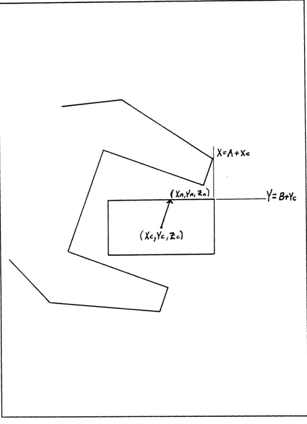
The most basic nonsymmetric touching conditions are
rectangular conditions. Figure 8 shows two-dimensional rect-angular conditions for the rectangle described by length 2A,
height 2B and center (Xc,Yc). If the center of the tongs is
given by (Xt,Yt) in the object reference frame, then the
object is within the tongs if:
IXt-XcJ <A
and
JYt-Yc
<B
If the object is within the tongs, it is then necessary to
check to see if the tongs are sufficiently closed. Let the
vector (Xn,Yn) be the normal vector to the face of the jaws.
If origin for the normal vector is taken to be the center of
the rectangle, it can be scaled to a new vector (Xs,Ys)
which intersects the surface of the intersects the rectangle.
If this vector were to intersect the line Y=B, then by
X= A+xe
Y_-8tYo
(Xs,Ys)=(A,YnA/Xn)
If the vector were to intersect the line X=A, its coordi-nates are given by:
(Xs,Ys)=(XnB/Ys,B)
The shorter of the two vectors is the one which stops at the
surface of the rectangle and its magnitude corresponds to
width of the rectangle as measured in the direction of the
normal vector. The tongs are closed enough to grasp the ob-ject if the closure D is less the the magnitude of the vec-tor (Xs,Ys).
EQUIPMENT
The major equipment used in this project is shown in figure 9. The simulation was run and controlled from the computer terminal in the center of the picture. The display
terminal is setting on the table to the far right. The
master manipulator is directly in front of the display ter-minal. The slave is in the background on the left. The large
rack of electronics behind the display terminal is the
servo-amplifiers and control interface. The computer is not
shown.
PDP11/34 Computer
The simulation was performed on a PDP11/34 running a RSX-11M operating system. This is a multiuser, timesharing
system. A PDP11/34 is not a particularly fast computer, how-ever it was sufficient. It would be more desirable to run on
LiPUIIU-·i-a mLiPUIIU-·i-achine solely dedicLiPUIIU-·i-ated to this tLiPUIIU-·i-ask. E-2 Master-Slave Manipulator
The manipulator was a rebuilt Argonne National Labor-itory E2 master-slave manipulator (2). This is a light hot-room style manipulator with seven degrees-of-freedom and full force reflection. It is electronically coupled allowing it to be interfaced to the PDP11/34 through a AN5400 A/D converter using an interface built by K. Tani (7). The con-trol interface allows independent sensing and control of each degree-of-freedom. Figure 10 show the E-2 slave manip-ulator simulated in this project.
Megatek Display Processor
The graphics were performed on a Megatek 7000 vector graphics terminal with three dimensional hardware rotate and a resolution of 4095 lines. The display processor has the ability to move the beam from its last location to a new location on the screen with the beam either on or off. The beam can also be moved a given displacement from its last position. With appropriate manipulation, text strings can be displayed in a variety of sizes and orientations. A series of commands can be defined to be a subpicture. The commands can then be executed by referencing the subpicture number. This allows a series of strokes which is used many times to be defined only once, then accessed by a single command.
This saves time in loading the display processor.
-45-The hardware rotate is a 4x2 matrix multiplier which is loaded into the display list and affects all succeeding vectors. It is capable of rotation, translation, scaling and clipping at screen boundaries. It is not, however, capable of perspective. The origin for all transformations is as-sumed to be the center of the .screen. Calls to the hardware rotate are not cumulative, but rather each call overrides the preceeding call. Relative vectors are affected by the
rotation matrix applied to t
ceeding the relative vectors
multiplier was called. This
the sphere which was made up s The above commands are block in the PDP11/34 and are display list en masse by a DMA tially scans the display list on the display monitor. There the location of a particular list and commands to change commands can be erased from t
he first absolute vector pre-regardless of when the matrix caused some problems in moving olely of relative strokes.
placed in an installed common transferred to the Megatek's transfer. The Megatek sequen-and puts the desired vectors are also commands to determine instruction in the the display that location. Any number of he end of the display list and be replaced by others.
EXPERIMENTAL DESIGN Programming Considerations
There are two important, competing programming
fac-tors in the simulation: speed and size. The RSX11M system
-47-which was operating on our machine restricts program size to
32K words. A 4K address window is required for each
instal-led common block used in a program. One common block was
needed to communicate with the A/D and Megatek, and one
common block was needed to hold Megatek commands prior to
DMA transfer. This means the maximum effective program size
was only 24K. Speed was a factor since it was desirable that
the program run in real time. It was particularly critical
when the program ran simultaniously with H. Kazerooni's dynamics program, which required a cycle time of less than 230 milliseconds to retain stability. Secondly, when com-puter generated force-feedback was desired, the computer needed to send signals to the manipulator control interface at time intervals on the order of 20 milliseconds.
Most of the graphics program was involved in calcu-lating rotation matrices and manipucalcu-lating objects. Only a small portion of the program was involved in initialization. This eliminated the possiblity of using overlays or multiple tasks to reduce program size. It was necessary to make com-promises between arrays versus explicit variables, and subroutines versus inline program segments. Explicit vari-ables and inline programming are faster, but require more program space. When there are many zero terms in a program section, such as those which occur when preforming multipli-cations of rotation matrices, explicit programming may be as
short as subroutines and obviously much faster. In general,
explicit variables and inline programming were used for
speed and ease of interpretation.
The amount of data space required was reduced by
placing all arrays in the unused portions of the common block associated with the display processor. All point data for the display was placed in direct access files, elimi-nating the need to bring it into the program. This also made program size independent of display complexity.
Using the display processor's hardware rotation and subpictures reduced cycle time by a factor of three over the equivalent program without these options. During the initial-ization segment of the program, each independent element of the display was drawn into a subpicture in its unrotated form. In the main body of the program, the display was created by loading the appropriate transformation matrix into the display processor's hardware rotate, followed by calling the desired subpicture. The use of subpictures re-lieved the computer from the task of reloading the entire display each program cycle. The hardware rotate eliminated the need to individually calculate the coordinates of each point in the display.
When the manipulator was allowed to move freely un-der computer control it was critical that the manipulator be controlled at regular time intervals. Since these intervals
-49-were shorter than the cycle time of the display program, control of the manipulator during free motion was performed by a separate program. When the manipulator was touching the simulated surface and force-feedback was being generated, the cycle time was not as critical because the velocity of the manipulator was small. Since in this case the display program needed to calculate the new angular position of the manipulator required to generate force-feedback, the display program controlled the arm while the control program re-mained dormant. Syncronization between the two programs was achieved by the use of flags passed through an installed common block.
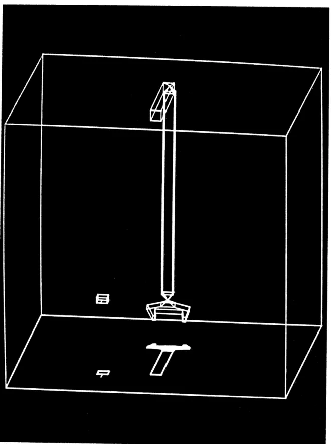
Manipulator and Vehicle Simulation
A design for the manipulator was chosen which simply but accurately represented the shape of the E-2 manipulator. Since no hidden line removal was attempted in order to keep the cycle time of the program down, too many lines would have made the display difficult to view. The tongs which are the most important portion of the display were given the most detail. The forearm and shoulder had a square, rather than circular cross-section. Cylinders are difficult to dis-play correctly unless complex algorithms are used to deter-mine the location of their edges. The square cross-section also gave a better perception of rotation of than a cir-cular cross-section.
Two types of objects and touching conditions were implemented. The first object implemented was a sphere using
spherical touching conditions. When this proved successful,
a rectangular peg was installed. The peg used two sets of
rectangular touching conditions. One for the main body of
the peg and one for the stem.
Various dynamic and static properties could bb inputted for the objects allowing a simulated environment to be built up within the computer. Gravity, drag, elasticity of collision, conservation of momentum and the hardness of the objects were all parameters which could be entered into the simulation. The manipulator and objects were enclosed within a rectangular room. When a moving object collided with a wall of the room, it rebounded off the wall. Aside from demonstrating conservation of momentum, the main pur-pose of the walls was to keep the objects within the reach of the manipulator.
Two applications of force-feedback were introduced. When an object was gripped by the manipulator, force-feed-back was sent to keep the tongs open to the width of the ob-jects. The resulting sensation was that of an actual object within the tongs. The second application involved applying force-feedback to the full manipulator. A three-dimensional surface was defined. The surface was assumed to be relative-ly flat eliminating the need to calculate the surface
nor-mal, instead the surface normal was assumed to be vertical.
Different hardnesses were assigned to various locations on
the surface. Force-feedback was implemented so that the
sur-face could be felt when it was touched by the manipulator.
As visual feedback, a gridwork approximation of the surface
was displayed on the graphics terminal. To aid the operator
in perceiving depth, the contour directly below the
manipu-lator was displayed in darker linework. As the manipulator
penetrated the surface, the contour deflected. The extent of the deflection was dependent on the stiffness of the surface
and depth of penetration. If the surface was soft,
deflec-tion only occurred in the neighborhood of the penetration.
If the surface was stiff, the whole surface deflected.
The simulation could be displayed from any viewpoint.
The viewpoint could be either stationary or moving. It has
been suggested that a moving viewpoint might be useful in
giving the operator a better perception of the
three-dimen-sional nature of the environment (6). The display could be
scrolled and zoomed so that any portion of the display could
be observed in detail. The viewpoint could be controlled
from the keyboard without interrupting the program by use of a request for IO0 (QIO).
The vehicle simulation was capable of the same
func-tions as the manipulator simulation. The manipulator was
degree-of-freedom motion. The position of the vehicle was inputted through an installed common block, which allowed the vehicle to be controlled by a secondary program.
Depth Indicators
A major difficulty associated with a vidio terminal is the lack of depth perception. Normally, when one is look-ing at a three-dimensional scene, one's brain generates the peception of three-dimensions from differences in parallax between the scene veiwed through the right and left eyes. The differences in parallax are associated with the distance between the two eyes and the distance between objects and the eyes. When a scene is displayed on a vidio terminal, all points are at the same distance from the eyes and the paral-lax information is lost.
When the simulation was first developed, depth in-formation was transmitted using the traditional orthographic projections. This approach appeared to cause some coordin-ation problems and the operator seemed to become confused over which view was the front and which was the side. Exper-ienced manipulator operators often rely heavily on shadows for depth cues. The second depth indicator was a shadow with the source of illumination directly overhead. The shadow was cast on a imaginary horizantal floor 50 inches below the manipulator's shoulder. Walls displayed on the screen were helpful in orienting the shadow. Both of these indicators
require extensive prior knowledge of the environment. The
third depth indicator was a proximity indicator. The
indi-cator showed the absolute distance between the tongs and the
object as a line on the display terminal. The display was
designed such that the length of the line was the same scale
as the display when the object was within 24 inches of the
tongs. The indicator was ten times less sensitive at longer
ranges. The proximity detector could be implemented by
placing a sonar device on the tongs of a manipulator.
Experimental Measurement of Operator Performance
The three depth indicators plus a control were
tested on five subjects. Two types of tasks were designed.
The first involved reaching out and grabbing a two inch,
stationary sphere. The time required for a subject to grasp
the sphere after the display was flashed on the screen was
recorded. In the second experiment, the task was the same
however the sphere was moving. The path of the sphere was
an orbit about the surface of an ellipsoid described by: X=Xc+10sin( t/3)cos(t/12)
Y=Yc+5sin(t/3)sin(t/12) Z=Zc+7cos(t/3)
where (Xc,Yc,Zc) was a vector describing the center of the
ellipsoid, t was the time in seconds and distances were
measured in inches. It was hoped that the moving task would
depth indicators.
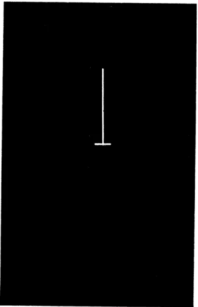
All three display types were shown at the same scale. The shadow was displayed along with reference walls at an azimuth and zenith of 15 degrees ( figure 11 ). The second display type was a front view with a proximity indicator displayed vertically above the manipulator ( figure 12 ). The third display type was a front and a side orthographic projection shown side by side (figure 13 ). The control was the proximity indicator with no view of the manipulator
( figure 14 ).
The subjects were run through a series of display types with both moving and stationary objects. The positions of the objects had to be selected such that the objects re-mained within the reach of the manipulator and did not coincide with any real object which would obstruct the mani-pulator. Display types were mixed because subjects tended to become bored with repetitions of the same display type. The order of the display types was kept constant so that the subjects knew which display type to expect next. The posi-tions of the sphere were arranged such that the average dis-tance between successive positions was the same for each display type.
RESULTS AND CONCLUSIONS Master-Slave Simulation
0 S 0 0 0
Figure 13 Display Type 3 Figure 14 Display Type 4