A comparison of washout filters using a human dynamic orientation model

A COMPARISON OF WASHOUT FILTERS USING A

HUMAN DYNAMIC ORIENTATION MODEL

by

Susan A. Riedel

B.S.. Massachusetts Institute of Technology (1976)

SUBMITTED IN PARTIAL FULFILLMENT OF THE REQUIREMENTS FOR THE DEGREE OF MASTER OF SCIENCE

at the

MASSACHUSETTS INSTITUTE OF TECHNOLOGY September, 1977

19

Depir): en of Aexrr Xn ics and Astronautics August 24, 1977 Certified by.

OW _{if Thesis Supervisor} Accepted by

A C014PARISON OF WASHOUT FILTERS USING A

HUMAN DYNAMIC ORIENTATION MODEL by

Susan A. Riedel

Submitted to the Department of Aeronautics and Astronautics on August 24, 1977, in partial fulfillment of the requirements

for the degree of Master of Science. ABSTRACT

The Ormsby model of human dynamic orientation, a discrete time computer program, has been used to provide a vestibular

explanation for observed differences between two washout schemes. These washout schemes, a linear washout and a nonlinear wash-out, were subjectively evaluated by Parrish and Martin. They found that the linear washout presented false rate cues, caus-ing pilots to rate the simulation fidelity of the linear scheme much lower than the nonlinear scheme. By inputting the motion histories from the Parrish and Martin study into the Ormsby mo-del, it was shown that the linear filter causes discontinuities in the pilot's perceived angular velocity, resulting in the sen-sation of an anomalous rate cue. This phenomenon does not oc-cur with the use of the nonlinear filter.

In addition, the suitability of the Ormsby model as a sim-ulator design tool was investigated. It was found to be a use-ful tool in predicting behavior of simulator motion bases, even when the mechanical motion base is replaced by a computer sim-ulation. Further investigation of the model could provide sim-ulation designers with a tool to predict the behavior of motion bases still in the drawing board stage.

Thesis Supervisor: Dr. Laurence R. Young Professor of Aeronautics

ACKNOWLEDGEMENTS

I wish to express my heartfelt thanks to Professor Laurence R. Young, whose guidance and teaching were a con-stant source of encouragement throughout this work.

I would also like to thank Russell Parrish and Dennis Martin, Jr., whose preliminary work on the washout schemes at Langley set the stage for this thesis.

This work would not have been possible without Dr. Charles Ormsby, the person responsible for the

physiologi-cal model used for the analysis of the washout schemes. Additional thanks go to Josh Borah, whose documenta-tion of the Ormsby model is the basis for the appendix to this thesis; to Ginny Spears at Lincoln Laboratory and Mike Hutchins at Draper Laboratory who provided invaluable

assistance in preparing the data for use on the Man-Vehicle Laboratory computer; and to my friends who read and

comment-ed on the manuscript at various stages of completion.

Finally, I would like to dedicate this thesis to my fam-ily. The loving and supportive environment which they

This thesis was supported by NASA grants NGR 22-009-701

TABLE OF CONTENTS

CHAPTER NUMBER PAGE

Introduction 14

1.1 The Physiology of Motion Simulation 16 1.2 The Use of Washout and Visual Cues

in Simulation 17

1.3 Thesis Ob'jectives and Organization 18...

II The Washout Filters 20

2.1 The Linear Washout 21

2.2 The Nonlinear Washout 26

2.3 A Comparison of Washout Schemes 28 2.4 Empirical Comparison of Washout

Filters 33

III The Physiological Model 44

3.1 The Human Vestibular System 45

3.2 The Ormsby Model 51

IV Data and Results 63

4.1 Data Description 63

4.2 Aileron Roll Cues 68

4.3 Aileron Yaw Cues 73

4.4 Rudder Roll Cues 77

4.5 Rudder Yaw Cues 81

V Conclusions 89 5.1 The Vestibular Explanation Question 90 5.2 The Suitability as a Design Tool

Question 94

5.3 Suggestions for Further Research 98

APPENDIX 100

A.l Human Dynamic Orientation Model 100

A.2 Subroutine STIM 113

A.3 Subroutine DOWN 118

A.4 Subroutine Library 123

A.5 Kalman Gains Subroutines 133

A.6 Kalman Gains Subroutine Library 138

TABLE OF FIGURES

FIGURE NUMBER

Block diagram for Schmidt washout scheme.

Block diagram for Langley out scheme.

Block diagram for Langley washout scheme. and Conrad linear wash-nonlinear 2.1 2.2 2.3 2.4 2.5 2.6 Time histories eron inputs. Time histories on inputs. Time histories der inputs. Time histories inputs.

of roll cues for

ail-of yaw cues for

ailer-of roll cues for

rud-of yaw cues for rudder

23

25

27 29

31

Design concept for digital controller.

Amplitude and phase plots fot three types of washout filters.

First-order linear and nonlinear ada-ptive washout response to a pulse in-put.

Time histories for throttle inputs.

Time histories for column inputs.

2.7 2.8 2.9 2.10 2.11 2.12 32 35 37 38 40 41 42 PAGE

3.1 Horizontal semicircular canal. 46

3.2 Orientation of semicircular canals. 47

3.3 Cross section of otolith. 49

3.4 Orientation of otoliths. 50

3.5 Afferent model of semicircular canals. 52

3.6 Afferent model of otolith system. 53

3.7 DOWN estimator. 57

3.8 Angular velocity estimator. 59

3.9 Overview of Ormsby model. 61

4.1 Commanded inputs to simulation. 66

4.2 Perceived angular velocity for simulated

linear aileron roll cue input. 69

4.3 Perceived angular velocity for simulated

nonlinear aileron roll cue input. 70 4.4 Perceived angular velocity for commanded

aileron roll cue input. 71

4.5 Perceived angular velocity for simulated

linear aileron yaw cue input. 74

4.6 Perceived angular velocity for simulated

nonlinear aileron yaw cue input. 75

4.7 Perceived angular velocity for commanded

aileron yaw cue input. 76

4.8 Perceived angular velocity for simulated

Perceived angular velocity for simulated nonlinear rudder roll cue input.

Perceived angular velocity for commanded rudder roll cue input.

Perceived angular velocity for simulated linear rudder yaw cue input.

Perceived angular velocity for simulated nonlinear rudder yaw cue input.

Perceived angular velocity for commanded rudder yaw cue input.

Perceived angular velocity aileron yaw cue inputs.

Perceived angular velocity rudder yaw cue inputs.

Perceived angular velocity aileron roll cue inputs.

Perceived angular velocity rudder roll cue inputs.

for three for three for three for three 4.9 4.10 4.11 4,12 4.13 79 80 82 83 84 5.1 5.2 5.3 5.4 91 92 95 96

TABLES

2.1 Pilot evaluation of motion cues for

linear and nonlinear washout schemes. 34

4.1 Variables recorded during simulation

runs. 64

4.2 Data used as input to Ormsby model. 67

A.l Variables used in main program. 108

A.2 Variables output from model. 112

A.3 Twelve test cases used in STIM. 115

A.4 Variables used in STIM. 116

A.5 STIM variables and printout variables. 117

A.6 Variables used in DOWN. 121

A.7 Otolith state equations. 130

A.8 Canal state equations. 131

LIST OF PARAMETERS

a translational acceleration

A acceleration vector

DOWN perceived vertical vector

f specific force

F specific force vector

FR firing rate g gravity vector G gravity vector n afferent noise p roll rate q pitch rate r yaw rate R rotation vector

SF specific force vector SFR spontaneous firing rate

x longitudinal axis y lateral axis z vertical axis 6 change in setting 0 pitch angle yaw angle

4'

LIST OF SUBSCRIPTS AND SUPERSCRIPTS

a aircraft

c centroid coordinate system

d washed out variable

e elevator

H high frequency component HD head coordinate system i inertial coordinate system L low frequency component

oto otolith r rudder ssc semicircular canals T throttle tot total x longitudinal axis y lateral axis z vertical axis

CHAPTER I INTRODUCTION

For many applications it is often desirable to simulate

a particular vehicle motion without using the actual vehicle:

* The Federal Highway Department sponsors many drunk driver studies. In order to insure the

safety of the driver, the vehicle and the

ex-perimenters, these experiments are often

car-ried out in a moving base simulation of an automobile.

*The U.S. Navy has commissioned studies of the habitability of large high-speed

surface-eff-ect-ships. It is necessary to understand to

what extent crews will be able to function on these ships even before a prototype is built.

This research is carried out on a motion

gen-erator, which simulates the expected range of motion of these ships (7].

*The U.S. Air Force makes extensive use of both stationary and moving base aircraft simulators

in pilot training programs. Simulators

pre-sent no risk to the pilot, and avoid the costs

of fuel and repair or possible loss of an

air-craft.

The above examples illustrate three of the many possible

uses of simulators - to carry out driver-vehicle studies with-out using an actual vehicle, to predict crew habitability on

board a ship not yet built, and to train aircraft pilots

with-out risking the pilot or the plane. As vehicles become

in-creasingly complicated, and costs continue to rise, motion

simulation takes on a new importance.

There are many types of cues a person uses to sense motion.

The basic inputs are specific force and angular acceleration,

which can influence the vestibular system in the inner ear, the

tactile sensors at points of contact with the vehicle, and the

proprioceptive sensors as muscles are -stretched and compressed.

In a simulator, it is not always possible to reproduce a

par-ticular motion history exactly. Often, some cues can be

pre-sented only at the expense of neglecting other cues. The basic

goal in motion simulation is to arrive at a compromise in

101 The Physiology of Motion Simulation

Simulation technology now makes heavy use of digital

computers to present as much of the motion cue as possible.

High speed processing allows the use of very complex linear

filtersand recently, of nonlinear adaptive filters.

Micro-processor technology has also made much of the slower

elec-trical circuitry obsolete.

But the goal of simulation has not really changed - try to present as many of the specific force and angular

acceler-ation cues as possible, without exceeding the constraints of

the simulator [18]. This has always been the most

straight-forward approach, since it is the specific force and angular

acceleration cues which are most readily available.

Once a good understanding of the physiological aspects

of motion simulation is attained, a physiological model of the

human operator will be a valuable tool in simulator design.

The comparison of actual motion and simulated motion using such

a model would be useful in determining the realism of the

sim-ulation in a quantitative way. This model would also be

help-ful in comparing two different simulation schemes, providing

1.2 _{The Use of Washout and Visual Cues in Simulation}

Constraints in position, velocity and acceleration of a

simulator limit the capability of producing a desired motion

exactly. The problem is to present the sensations of a wide

range of motion, and to do this in a very limited space. This

problem is solved with the use of washout filters in each axis of motion, in order to attenuate the desired motion until it

falls within the constraints of the simulator.

An important aspect of motion simulation has not yet been

mentioned - the visual cues available to detect motion. Peri-pheral visual cues seem to be most important in presenting the

sensation of motion. The peripheral field may be stimulated

by a moving pattern of stripes or dots, or by an actual "out -the - window" cockpit view [2,5].

Taken together, washout filters and visual stimulation perform the function of simulation in which motions seem to go

beyond the constraints of the simulator. The motion is

dupli-cated to the point of constraint in a given axis. Then the

wash-out filter takes over and attenuates the motion to meet the

constraint. Meanwhile, the visual field is stimulated so as to

give the impression of continued motion, motion beyond the

cap-abilities of the simulator. In this way, a wide range of mo-tions can be simulated using a very restricted motion base.

1.3 Thesis Objectives and Organization

It is obvious from the previous discussion that the

wash-out filters in a simulator are critical to the fidelity of the

simulation. The research leading to this thesis compares two

different types of washout filters currently in use, in order

to quantify the differences between them. The means of

com-parison is a physiological model of human dynamic orientation,

based largely on the known physiology of the vestibular system.

This work attempts to answer a specific question and a general

question:

* Can the observed differences in simulation

fidelity between the two filters be

explain-ed using a physiological model of human

dy-namic orientation?

*What are the implications for this model as

a drawing board tool in simulator design?

Chapter II presents the two washout filters in detail, and

discusses the previous work which led to the research

present-ed in this thesis.

Chapter III describes the human vestibular system and the

model of human dynamic orientation developed by Ormsby.

Chapter IV describes the data in this work, as input to

the model, and then presents the perceived angular velocities

Finally, Chapter V presents the conclusions which can be

drawn from the results presented in Chapter IV, in light of

the questions posed in the above- section. Also included are

CHAPTER II THE WASHOUT FILTERS

The two washout filters of interest in this comparitive

study are the following:

* A linear filter, essentially a Schmidt and Conrad

coordinated washout 116,17].

* A nonlinear filter, coordinated adaptive washout.

Basically, the two filters are versions of Schmidt and Conrad's

coordinated washout. This scheme uses washout filters in the

three translational axes, and only indirectly washes out the

angular motion. The primary difference between the linear and

nonlinear schemes is in the type of translational washout

fil-ters employed. The linear scheme uses second-order classical

washout filters in the three axes, while the nonlinear scheme

uses coordinated adaptive filters for longitudinal and lateral

washout and digital controllers for vertical washout. These

schemes differ in their presentation of the rate cues, for a

pulse input. The linear scheme presents an anomalous rate cue

when the pulse returns to zero. This behavior is not observed

The next two sections discuss the filters in greater

de-tail. The final sections present the differences between the

filters and the results of a previous subjective analysis of

the washout schemes.

2.1 The Linear Washout

The purpose of washout circuitry is to present

transla-tional accelerations and rotatransla-tional rates of the simulated

air-craft. It is necessary to obtain coordination between

trans-lational and rotational cues in order to accomplish certain

motion simulations:

* A sustained horizontal translational cue can

be represented by tilting the pilot. The

gravity vector is then used to present the

cue. But in order to make this process

be-lievable, the rotation necessary to obtain.

the tilt angle must be below the pilot's

ab-ility to perceive rotation. The solution is

to start the cue with actual translational

motion of the simulator until the necessary

tilt angle is obtained. In this manner, the

pilot will sense only translational motion,

long after such motion has actually ceased.

* In a similar sense, it can be seen that a de-sired roll or pitch cue cannot be represented

by means of rotation alone. This would result in a false translational cue, because the

gra-vity vector is misaligned. In order to present

a rotational cue, translational motion must be

used at the start, to offset the false

trans-lational motion cue induced by the rotation.

The two cases above clearly illustrate the need for

coor-dination in translational and rotational motion. Schmidt and

Conrad's coordinated washout scheme fulfills this need.

Fig-ure 2.1 presents a block diagram illustrating the basic

con-cepts.

The desired motions of the simulated aircraft are

trans-formed from the center of gravity of the aircraft to the

cen-troid of the motion base. This transformation provides the

de-sired motion at the pilot's seat. The motions of the base are

based on the desired motions of the centroid.

Vertical specific force is transformed to vertical

accel-eration *d by use of a second-order classical washout filter.

The longitudinal and lateral accelerations are also obtained

from the longitudinal and lateral specific forces. First, these

specific forces are separated into steady-state and transient

parts. The steady-state part of the cue is obtained from a

tilt angle to align the gravity vector. The transient part of

the cue is transformed into the longitudinal acceleration, *d' and the lateral acceleration,

yd,

SIMULATED AIRCRAFT CENTER OF GRAVITY TO SEAT TO CENTROID TRANSFORMATION

I1

_CW

_x

TALO TILT SEPARATION, ANGULI AL WASHOUT f

A iy ELIM. FALSE TRANS. WASHOT

BRAKING VELOCITY AND PREDIC-ACCELERATION POSITION LIMITS

xa ya Z AR UT LEAD NSATION COMPENSATION ACTUATOR EXTENSION TRANSFORMATION MOTION BASE

Figure 2.1 Block diagram for Schmidt and Conrad washout

scheme (17]

f

LEAD COMPE

washout filter.

Braking acceleration is then used to keep the motion

with-in the prescribed position, velocity and acceleration limits

of the motion base.

The rotational degrees of freedom are only indirectly

washed out through elimination of false g cues. Rotational

rate cues are represented by angular and translational motion,

just as longitudinal or lateral cues. But in this case, the

translational motion is used only to eliminate the false g cue

induced by rotational movement, and thereby makes no direct

contribution to the rotational cue.

After the six position commands (x d'dfzd,,, are

ob-tained from the washout circuitry, lead compensation is

pro-vided to compensate for servo lag of the base. The actuator

extension transformation is then used to obtain the correct

actuator lengths used to drive the motion base.

The actual filter evaluated in this work is a Schmidt and

Conrad coordinated washout, adapted by Langley Research Center

[14]. The major difference is that the Langley washout is

car-ried out in the inertial reference frame, rather than the body

axis system. A block diagram of this filter is shown in Fig-ure 2.2.

1

,

e$

BODY TO INERTIAL TRANSLATIONAL

TRANSFORMATION WASHOUT * ** F ixF iyF iz SIGNAL _BRAKING SHAPING ACCELERATION NETWORK CIRCUIT jT 6T T Rd d 2d A JINERTIAL TO BODY TRANSFORMATION a ra p'

q

*

Figure 2.2 Block diagram for Langley linear washout Lcheme [13]

2.2 The Nonlinear Washout

The nonlinear filter of interest here is again essentially

a Schmidt and Conrad coordinated washout. The difference

be-tween the nonlinear Langley filter and the Schmidt and Conrad

filter are that the Langley filter uses the inertial reference

frame rather than the body axis system, and nonlinear filters

are used for the washout rather than the linear filters used

by Schmidt and Conrad. Hence, the designation "nonlinear wash-out" is used.

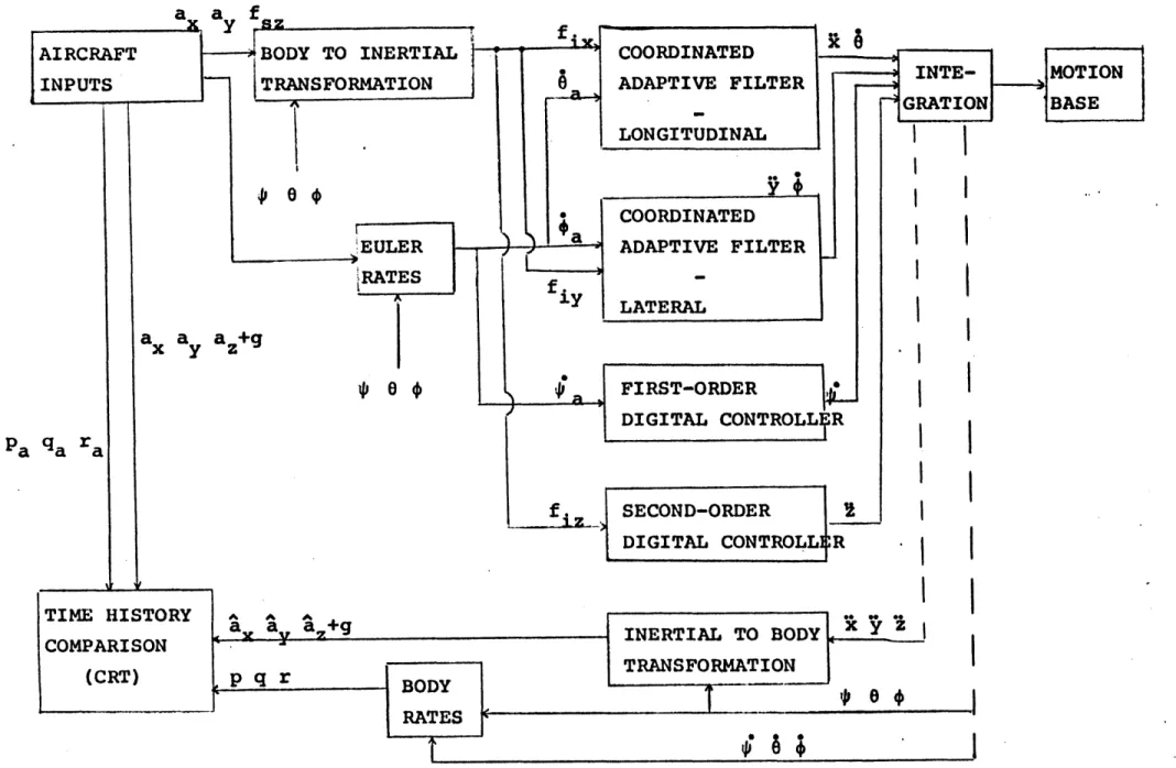
Figure 2.3 presents a block diagram for this nonlinear

scheme. It is seen that two different types of nonlinear

fil-ters are used - coordinated adaptive filters for longitudinal and lateral cues, and digital controllers for vertical cues.

These two types of filters will be discussed in turn.

Coordinated adaptive filters [11] are based on the

prin-ciple of continuous steepest descent. They are used in this

washout scheme to coordinate surge and pitch in presenting the

longitudinal cues, and sway and roll in presenting the

later-al cues. Derivation of these filters can be found in the

liter-ature [11,12]. Basically, they perform the same functions as

the second-order classical filters used by Schmidt and Conrad

by providing translational specific force cues and rotational rate cues.

Digital controllers, the second type of nonlinear filters,

INPUTS TRANSFORMATION

ra-4cc

10

0

*

i e

I

Figure 2.3 Block diagram for Langley nonlinear washout scheme [131

GRATION BASE FR JR-a qa ra g~3 TIME HISTORY COMPARISON (CRT) r I I T

first-order digital controller provides the yaw rate cue, while

a second-order controller provides the vertical specific force

cue. These filters are designed to present as much of the

on-set cue as possible before switching to the washout logic.

Figure 2.4 illustrates the design concept for a

first-order digital controller. From 0 to T the controller presents

a scaled version of the commanded input. AtT1 a linear decay

is applied to reduce the command to the motion base constraint

value, B. Washout then occurs at the constrained value, unless

another input is commanded, -as at T2.

The second-order digital controller used for the vertical

specific force is similar, although mathematically more

complex.

2.3 A Comparison of Washout Schemes

Essentially, the two washout schemes of interest are

Schmidt and Conrad washouts. The so-called linear washout

contains second-order classical washout filters which

trans-form the specific forces in each axis to translational

accel-erations in each axis. The Langley washout performs these

transformations in the inertial frame rather than the body

axis frame used by Schmidt and Conrad.

The nonlinear washout scheme uses two types of nonlinear

filters to provide the translational acceleration cues. A coordinated adaptive filter is used to coordinate surge and

MAX ; d a deg/sec 0

I

1

1

1

/

1

I

I

f

I

Figure 2.4 Design concept for digital controller [11]

MAX -deg A DB 0 I

I

pitch for longitudinal cues, and sway and roll for lateral

cues. A digital controller is used for the uncoordinated heave and yaw motions. Again, the Langley nonlinear scheme

washes out in the inertial frame.

In Figure 2.5, amplitude and phase versus frequency is

shown for the three types of washout filters - linear, adaptive and digital controller. Both the first-order and second-order

cases are shown. The motion base characteristics are the same

in all cases. Since the amplitude and phase response of the

nonlinear adaptive filter changes with the magnitude of the

in-put, the worst case for the nonlinear filter is presented here.

As is shown, the digital controller has the best response

char-acteristics, and the adaptive filter is better than the linear

filter. This holds true for both the first- and second-order

cases.

In terms of motion cues, there is a fundamental difference

between the linear filter and nonlinear filter for the

first-order case. Figure 2.6 shows the response of the two filters

to a pulse input. The difference between the filters is the

anomalous rate cue presented by the linear filter as the pulse

input returns to zero. This false cue is most noticeable for

pulse-type inputs, and disappears as the input becomes

sinu-soidal. Since the differences between the linear and nonlinear

filters vary with input, performance of a given filter is

1.C10 100 .o8 80 AMPLI- AMPLITUDESE TUDE .6- 60 LHADE RATIO LEAD RA.I 4 - PHA SE 40 d eg .2 20 0 First-order filters Second-order filters 00 ,8- 60 AMPLI- AMPLITUDE TUDE .6 - -20 RATIO PHASE 4 PHASE -30 LEAD deg .2 10 0 0 1 2 3 4 5 FREQUENCY rad/sec Linear filter Adaptive filter Digital controller

Figure 2.5 Amplitude and phase plots for three types of filters [1]

LINEAR

FALSE CUE

;NON-LINEAR

Figure 2.6 First-order linear and nonlinear adaptive response to a pulse input [13]

2.4 Empirical Comparison of Washout Filters

Parrish and Martin, the major investigators of these two

washout schemes at Langley, devised a subjective test to

deter-mine the differences between the two filters in actual

simula-tion [13]. Seven pilots flew a six-degree-of-freedom simulator

equipped with both linear and nonlinear washout schemes. The

pilots were asked to rate the motion cues presented by each

scheme for throttle, column, wheel and pedal inputs about a

straight-and-level condition ddring a landing approach.

The results of this evaluation process are presented in

Table 2.1. Each pilot determined his own criteria for

evalua-tion. In addition to rating the cues for each input, the pilots

were asked to rate the overall airplane feel - that is, how successful the overall motion was in representing the actual

airplane. In the table, the open symbols represent the rating

of the linear method, while the solid symbols represent the

rating of the nonlinear method. The washout methods were

ap-plied to a 737 CTOL aircraft simulation, and four of the pilots

(represented by the triangular symbols) had previous 737

cock-pit experience.

The pilot ratings for the throttle input are the same for

each method, as shown in Table 2.1. Even given the methods

back to back for comparison, the pilots could not detect that

a change had been made. Figure 2.7 shows the time histories

accelera-RATING _{HALF HALF HALF HALF}

UN-EXC. - GOOD - FAIR - POOR -

CCEP-WAY WAY WAY WAY ABLE

INPUT v &90 ₄ 00 THROTTLE O e

A

L 2

Table 2.1 Pilot rating filters [13]

45

3C

Tt

Throttle input 1

4-Commanded input to motion base

10--r

10- Linear washout response

10--10

0 5 10 15

TIME sec

Nonlinear washout response

Figure 2.7 Time histories for throttle input 6dT deg ea deg/sec q deg/sec q deg/sec 20 I i I I I

tion and pitch rate are the inputs to the washouts from the

simulated aircraft for such a maneuver. The figure shows very

little difference between the washout schemes, as the pilot

ratings indicated. The fundamental difference between the two

pitch rate filters is obscured in order to correctly represent

the decrease in longitudinal acceleration at six seconds.

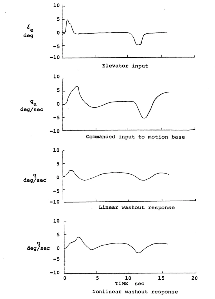
An elevator doublet was input to rate the motion cues for

a column input. Again, the pilots found little difference

be-tween the linear and nonlinear washout schemes, as shown in

Table 2.1. Four pilots rated the filters the same, while the

other three rated the nonlinear filter slightly higher. The

time histories for the elevator inputs are shown in Figure 2.8.

As in the throttle input case, the fundamental difference

be-tween the pitch rate filters is not apparent, due to the

coor-dination between pitch rate and longitudinal acceleration. In

addition, the pitch response of the 737 is not at all

pulse-like, which lessens the difference in performance of the filters.

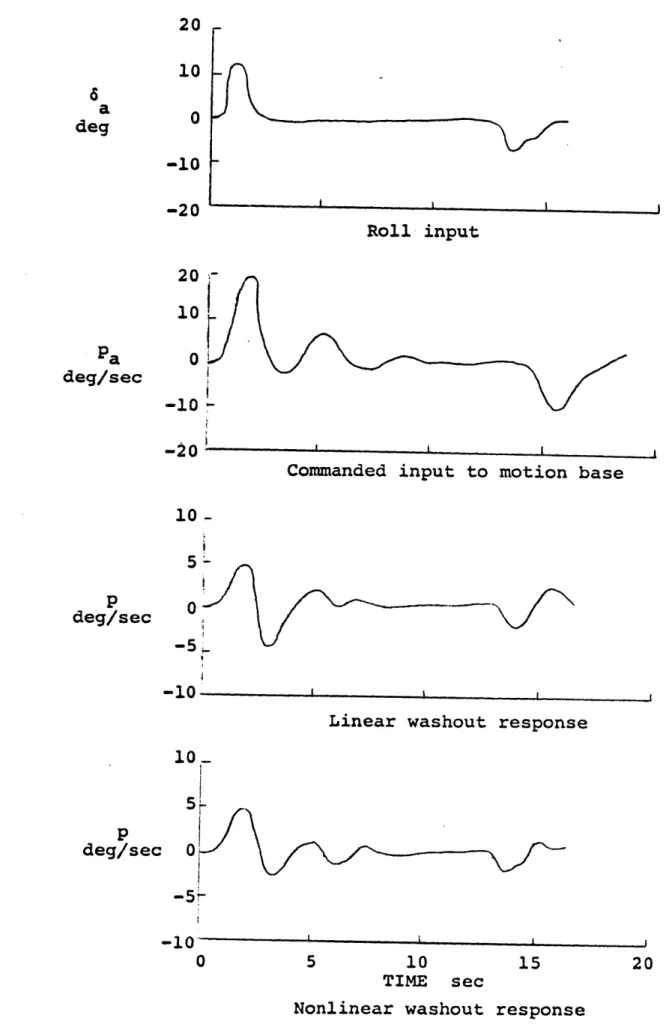
Wheel inputs were evaluated using ailerons to bank the

simulator 200 for a 300 heading change with a return to

straight-and-level flight. The pilots preferred to separate the wheel

inputs into roll cues and yaw cues to evaluate these cues

in-dividually. Figure 2.9 shows the time histories for roll cues

in the maneuver described. The anomalous rate cue is present

for the linear washout. This is reflected in the pilots'

5 0 -5. 10 10 5 AI

Commanded input to motion base

-I

Linear washout response

10 5 0 -5 -10 0 5 10 TIME sec 15 20

Nonlinear washout response

Figure 2.8 Time histories for column input e deg Elevator input da deg/sec 0 -5 -10 0 n 5 0 q deg/sec -5 -10 q deg/sec --

I

I

-101-Yaw input

Commanded input to motion base

0

Linear washout response

5 10

TIME sec

15

Nonlinear washout response

Figure 2.10 Time histories of yaw cues for aileron inputs

ar

filter to be at least one and one-half categories higher than

the linear filter.

Figure 2.10 shows the time histories for yaw cues during

the same aileron maneuver. Again, the anomalous rate cue is

present for the linear filter scheme. The pilots were

parti-cularly aware of a negative rate cue when the simulated

air-craft rate returned to zero during maneuvers of this type.

The ratings in Table 2.1 are at least one category higher for the nonlinear scheme, reflecting the unnateral feel of the

linear rate cue.

Each pilot flew a set of rudder maneuvers for both

wash-outs to evaluate roll and yaw cues. There were no changes in

the ratings from those obtained using the wheel. This is

re-flected in the time histories for roll and yaw, shown in

Fig-ures 2.11 and 2.12, respectively.

Finally, each pilot was asked to rate the two washout

schemes in terms of overall airplane feel. Table 2.1 shows

the large contribution made by roll representationin the

over-all airplane simulation. All pilots rated the nonlinear

wash-out at least one and one-half categories higher than the

lin-ear washout. They specifically objected to the anomalous rate

cue presented by the linear filter in both roll and yaw.

From this study, Parrish and Martin concluded that the

non-linear washout scheme better represents actual airplane motions

10 0 -20 Roll input ePa deg/sec p deg/sec 2o 10 0 -10 -20

Commanded input to motion base

10-5

0 -5

-10 wr

Linear washout response 10-p deg/sec 0 -10 0 10 TIME sec

Nonlinear washout response

Figure 2.9 Time histories of roll cues for aileron inputs 6 deg 5 15 20

YA ,

10-r 0-deg -10--?2 d Roll input 2C-10 deg/sec -20

Commanded input to motion base

1-p C

deg/sec

-10 I

Linear washout response

10-p deg/sec -10 0 5 10 15 20 TIME sec

Nonlinear washout response

10 0 6 r deg -2 Yaw inputs 20 10 0 -10 liI

Commanded input to motion base

10

5

0

-1 0 w r

Linear washout response

10 5 0 -5 -10 0 5 10 TIME sec 15 20

Nonlinear washout response

Figure 2.12 Time histories of yaw cues for rudder inputs ra deg/sec r deg/sec r deg/sec -10

I

sense. It appears that the nonlinear scheme does not present

more of the motion cue; it merely eliminates the false cue

pre-sent in the use of the linear washout.

The work presented in this paper attempts to quantify the results obtained in the subjective analysis made by Parrish

and Martin. In order to accomplish this, the motion histories

from the Parrish and Martin study are input to a model of human

dynamic orientation. The output from the model will provide

a vestibular explanation for the sensation differences between

the two filters. Results of this work are presented in

CHAPTER III

THE PHYSIOLOGICAL MODEL

A model which predicts human perceptual response to mo-tion stimuli has been developed at M.I.T.'s Man-Vehicle

Labor-atory by Ormsby (10]. The model, which exists as a FORTRAN

com-puter program, is based on the known physiology of the

vesti-bular system. While little is known about the processing of

the specific forces and angular accelerations received from the

vestibular organs, the simplifying assumptions made about this

process produce a model which agrees with available

neurologi-cal and physiologineurologi-cal data.

This chapter first presents an overview of the vestibular

system, and then goes on to discuss the mathematical modelling

of the system which leads to the current FORTRAN model. More

detailed descriptions of the vestibular system may be found in

the literature [9,15,19,20]. The complete derivation of the

model of human dynamic orientation is found in Ormsby. And a

description of the actual FORTRAN programs and their use is

3.1 The Human Vestibular System

The vestibular system, or labyrinth, comprises the non-auditory portion of the inner ear. It is composed of three semicircular canals, one utricle and one saccule in each ear.

The semicircular canals are the rotational motion sensors. They consist of three approximately orthogonal circular tor-oidal canals. The canals are filled with a water-like fluid

called endolymph. When the head undergoes angular

accelera-tion, the endolymph tends to lag behind the motion of the canal walls. The motion of the endolymph relative to the canal walls displaces the cupula, a gelatinous mass which completely

ob-structs one section of the canal called the ampulla. Sensory

hair cells embedded at the base of the cupula detect its

dis-placement. As a result, the deformation of the cupula is

trans-formed into an afferent firing rate which provides a signal of

rotational motion to the central nervous system (see Figure 3.1).

In a particular canal, all of the hair cells have the same polarization. When the flow of endolymph displaces the cupula

in a single direction, the hair cells are either all excited

or all inhibited. As shown in Figure 3.2, the canals on either side are essentially coplanar with the other side. Thus, they

are pairwise sensitive to angular accelerations about the same

axis. Since a pair of canals which are sensitive about the

high-UTRICLE AMPULA CUPUjLA CRISTA .ILARIS SENSORY HAIR C LS AFFERENT NERVE FIBERS

RP RS (X+) LS (Y+) .RP (Y-) LP (X-) RH (Z-) LH(Z+ KEY R RIGHT L LEFT H HORIZONTAL P POSTERIOR S SUPERIOR (X+) POSITIVE ACCEL-Z OUT ERATION ABOUT THE X OF PAGEJ X AXIS INCREASES THE

AF-FERENT FIRING RATE (Y-) POSITIVE ACCEL-ERATION ABOUT THE Y AXIS

DECREASES THE AFFERENT FIRING RATE

er processing centers respond to the difference in afferent

firing rates.

Two otolith organs, consisting of a utricle and a saccule,

are located in each ear. The otolith is sensitive to changes

in specific force. Figure 3.3 depicts the basic structure of

the otolith organs. The otolith consists of a gelatinous

layer containing calcium carbonate crystals, known as otoconia.

This layer is supported by a bed of sensory hair cells. An

acceleration of the head shifts the otoconia relative to the

surrounding endolymph, due to the higher specific gravity of

the otoconia. This shifting causes the sensory hair cells to

bend, sending a change in afferent firing rate through the

af-ferent nerve fibers to the central nervous system.

As shown in Figure 3.4, the utricles are oriented such

that their sensitivity is in a plane parallel to the plane of

the horizontal semicircular canals. The sensitivity of the

saccules is in a plane perpendicular to the horizontal canals.

The hair cells in the utricle are sensitive in all directions

parallel to its plane of orientation, while the hair cells in

the saccule make it predominantly sensitive to accelerations

SURROUNDING SENSORY OTOCONIA HAIR CELLS SUPPORTING CELLS AFFERENT NERVE FIBERS

UTRICLES

( U

SACCULES

Orientation of otoliths

3.2 The Ormsby Model

The mathematical model of the semicircular canals consists

of several parts. The first- part is the mechanical model of

the cupula deflection caused by motion of the endolymph. The

second part includes the interaction between the mechanical

movement and the afferent firing rate. The third part concerns

measurement noise, which is that portion of the afferent

sig-nal found to be independent of the mechanical stimulus input. Figure 3.5 depicts the afferent model of the semicircular canals as arrived at by Ormsby. Observation of cupula motion

led to the torsion pendulum model [9],' suggesting that the over-damped system reacts to angular velocity rather than angular

acceleration. The results of the model are expressed as a

transfer function of the following form:

FRc(s) ₌

(57.3)(300s 2)(.Ols+l) _W(S) (18s+l) (.005s+l) (30s+l)

+ SFR + n(t) (3.1)

s

The model of the otolith system is composed of two parts

- the mechanical model of the otolith sensor, and the

affer-ent response to otolith displacemaffer-ent. Figure 3.6 presaffer-ents the

afferent model of the otolith system used by Ormsby. The

me-chanical model of the otolith is that of a fluid-immersed mass

relat--. 09s (18s+l) (.005s+1) Torsion pendulum model 30s (.Ols+l) H F (30s+l) Mechanical

coupling _{Dynamics of most} rapidly adapting afferents + -+ Firing '0 -- Rate (ips) n(s) Afferent noise Displacement of endolymph Effective' displacement of hair cells Change in afferent firing

rate due to stimulus

w(s) = stimulus, angular velocity of head

Hi = Mechanical coupling of endolymph to effective hair cell displacement

F = Constant which relates hair cell displacement to change in firing

rate

SFR = Spontaneous firing rate of typical afferent cell (90 ips)

Figure 3.5 Afferent model of semicircular canals (after Ormsby [10])

W(s) tLJ I | i i I

SF

+

stimulus

M

C

of typical afferent cell

(90 ips)

Afferent Firing Rate (ips)

A n(s)

C Afferent

s _noise

echanical dynamics

of otoliths

Combined mechanical and afferent dynamics

Utricle A .2 B 91.1 C -46.1 Saccule .2 45.55 -23.05

ing afferent firing rate to specific force is:

FR 0(S) =(18000) (s+.1) SF(s) _{+ SFR + n(t) (3.2)}

(s+.2)(s+200) S

The input to the model consists of a stimulus composed of

specific forces and angular accelerations in each axis of the

head coordinate system. Each of these afferent inputs is the"

transformed into sensor -coordinates. From this sensor

stimula-tion, the afferent firing rates are derived, using the

trans-fer functions presented above.

At this point, the process becomes purely guesswork. Even

assuming that these afferent firing rates are available to some

central processing system in the brain, the form which this

processing takes is simply a guess. Ormsby guessed that the

central processor performs a type of least mean squares error

optimization to make an estimate of the specific force and

angular velocity inputs based on the afferent firing rates

out-put from the vestibular system sensors.

In this case, such a least mean squares estimator is a

Kalman filter (4,8]. The input is unknown except for an

pected range of magnitude and a frequency bandwidth, and an ex-pected measurement noise. Also, the input and the noise

stat-istics are time invariant, which makes the filter a

steady-state Kalman (or Wiener) filter. This steady-steady-state Kalman

and angular velocity from the afferent firing rates. These

estimates are tuned, using the Kalman filter gains, to yield

estimates which fit the available neurological and

physiologi-cal data for known inputs.

The filters used for canal processing are tuned such that

the estimates produced for the angular velocities are

essential-ly unchanged from the afferent inputs. This observation is in agreement with available data, suggesting that very little

central processing is performed. The otolith filters must be

tuned so that a more dramatic effect by the filters on the

aff-erent input is observed. This suggests that more central

processing is required, or that the model of the afferent

re-sponse is missing a term which has subsequently been

attribut-ed to the central processing mechanism in the tuning procattribut-edure.

Basically, the filter acts as a low pass filter with a time

constant of 0.7 seconds. The utricle and saccule differ only

in the Kalman filter gains, where the saccule gains are twice

the utricle gains.

Once the specific force and angular velocity estimates

have been obtained from the Kalman filters, the saccule

non-linearity must be accounted for. This is done by means of a

nonlinear input-output function, and allows the model to

in-clude observed attitude perception inaccuracies known as

Au-bert or Mueller effects [6]. The resulting specific force and

coor-dinates.

These estimates must now be combined to yield new estimates

of perceived position, velocity and acceleration. In the model

this is accomplished by a separate scheme, known as DOWN. DOWN

is a vector of length 1 g in the direction of perceived

ver-tical; as such, it is the model's prediction of the

perceiv-ed vertical. The basic assumptions used in combining the

spe-cific force and angular velocity estimates to arrive at DOWN

are the following:

* The system will rely on the low frequency

por-tion of the specific force estimates provided

by the otoliths.

" The system will use that part of the canal in-formation which is in agreement with the high

frequency content of the rotational

informa-tion provided by the otoliths.

This logic is presented in Figure 3.7. Block A produces

the estimate of rotational rate from the input specific forces

assuming SF is fixed in space. The low frequency component of

this estimate is filtered out in Block B. Block C isolates

the component of the low frequency angular velocity estimate

which is perpendicular to SF and DOWN. This is the mechanism discussed in Chapter II, which allows cancellation of canal

signals arising when prolonged rotations are stopped

W,

cL

H I

CALCULATE REDUCE ANGL

A N G L E 'B E T W E E N D ' -- -- - ,, D O W N

BETWEEN AND SF BY

D' AND _-At/T

SF gep

Figure 3.7 DOWN estimator [10]

YHD CONFIRMATION HD() GATE -_-F H ISOLATE 13F COMPONENT TO DOWN X1HD c G R A B L ISOLATE ssc ROTATE

YHD SF LOW PASS SF COMP. OFDOWN(t-At

FILTER TO HD BY R

ZH1D ) ~~~AND DOWN(t- t) Roto Rtot tot

;D' SF SF SF LN D'

vector which represents the low frequency rotational

informa-tion available from the otoliths (Roto)

Block D confirms whether or not the high frequency portion

of the canal rotational information is consistent with the high

frequency portion of the otolith rotational information. The

inconsistent part of the canal information is sent through a

high pass filter (Block E) and is then combined with the

con-sistent portion of the canal information. The component of

the resulting rotation vector parallel to DOWN is then

elimi-nated, leaving a rotational vector due to canal information

(Rsc). The total estimate of the rotation rate of the outside

world with respect to the last estimate of DOWN, Rtot, is

com-puted by subtracting Rssc from R oto. The net result of Blocks

H and I is to produce an estimate of DOWN which is the same as

the estimated specific force vector. This is accomplished by

a slow reduction in the discrepancy between SF and DOWN,

elim-inating any accumulated errors resulting from the integration

of rate information.

Figure 3.8 illustrates the model for predicting perceived

rotational rate. The angular velocity vector parallel to DOWN

becomes the perceived parallel angular velocity. The

perpen-dicular angular velocity is computed in three steps:

1. Calculate the difference between the com-ponent of angular velocity perpendicular

consis-WYHD M _WHD N '1z 1i DOWN COMPONENTS PARALLEL AND PERPENDICULAR TO DOWN bi~ K -> _ .I -I ________ L _HIGH PASS FILTER

III

Angular velocity estimator (10]

U' ~0 + w(t) +

ii

ii

tent with the rate of change of the

direc-tion of DOWN (Block K).

2. High pass filter this difference.

3. Combine the filtered result with the

DOWN-consistent angular velocity.

This process assures that the canals provide the high frequency

component of the rotational rate, while the low frequency

com-ponent is the rotational rate consistent with DOWN. The total

sense of rotation is thus the sum of the parallel and

perpen-dicular components.

This completes the description of the form of the Ormsby

model used in this work. A complete description of the model may be found in Ormsby's thesis. Figure 3.9 presents an

over-view of the entire model. At this point, a few important

ob-servations should be made:

*The Ormsby model was tuned using inputs with

known outputs for a certain set of discrete

time intervals - namely, an afferent update interval of 0.1 seconds and a Kalman filter

estimate update interval of 1.0 seconds. In

this thesis, due to the characteristics of the

input data, the afferent update interval is

0.03125 seconds, and the Kalman filter esti-mate update interval is 0.25 seconds. In order

RANSFORM CANAL DYN. OPT. ESTIM. RANSFORM 6HD ENSOR _*ZHD ENSOR rO HEAD x Equation 3.1 W& AFFERENT FIRING RATES Figure DOWN 3.7 IA ESTIMATC Ax -G + z

-OORDINAT UTRICLE DYN. OPT.ESTIM. _{OORDINAT S X D}

rRANSFORM RANSFORM F

JEAD TO -- jig),ICLE DYN. P.ETM --- A-ENSOR YHD

jSCO2EbN1OPT. ESTIM. _{r EDS}

SENSOR 20 HEAD SF SXCCUL E iY . OzP.72ESIM. IN Figure 3.8 ANGULAR VELOCITY W ESTIMATOR DO0W N +E E~ ) OTOLITH ESTIMATES

Figure 3.9 Overview of Ormsby model (after Borah [3])

G

I~-J

R

be retuned by changing the Kalman gains. This

process, which is necessary each time the update

intervals are changed, is described in more

de-tail in the appendix.

One important assumption made by this model is

that the inputs are unknown prior to their

pro-cessing. It was noted in the introduction to

this thesis that specific force and angular

ac-celeration act on the body as a whole,

provid-ing visual, tactile and proprioceptive, as well

as vestibular, cues. This model takes account

of the vestibular cues only, although the

tun-ing process may force it to consider certain

aspects of the other sensory cues. Thus, when

this model is applied to cases where the

sub-ject might have prior knowledge, or at least

an expectation of the motion, the results must

be interpreted in light of the limitations

im-posed by the model.

The Ormsby model of human dynamic orientation was used in

this work as a FORTRAN program implemented on a PDP 11/34.

The main program, as well as all associated subroutines, is

CHAPTER IV DATA AND RESULTS

As a logical consequence of the two previous chapters, it

is desirable now to evaluate the two washout schemes using the Ormsby model of human dynamic orientation. Such an evaluation

could serve the purpose of quantifying the differences between

the two filters which Parrish and Martin found in their

subjec-tive study. In addition, this evaluation could shed some light

on the question of the model's usefulness in simulator design.

This chapter presents the data used for this study, and

the results of the processing of the data by the Ormsby model.

4.1 Data Description

The data used in this work consists of four runs made

with a linear or a nonlinear washout on the Langley simulator.

These runs coincide with Figures 2.9, 2.10, 2.11, and 2.12.

Table 4.1 lists the definitions of the variables measured

dur-ing these simulation runs. Note that not only are the

simula-tor motions recorded, but also the commanded motions of the

simula-Table 4.1 Variables recorded during simulation runs VARIABLE TIME DELA DELE DELR THRIL PA PADOT QA QADOT RA RADOT AXA AYA PSIA THEA PHIA P Q R PDOTM QDOTM RDOTM AXCM AYCM PSIMB THEMB PHIMB XDDMB YDDMB DEFINITION time aileron deflection elevator deflection rudder deflection throttle input

roll rate of airplane

roll acceleration of airplane

pitch rate of airplane

pitch acceleration of airplane

yaw rate of airplane

yaw acceleration of airplane

longitudinal acceleration of airplane lateral acceleration of airplane

* of airplane

0 of airplane

0 of airplane

roll rate command to simulator

pitch rate command to simulator

yaw rate command to simulator

roll acceleration measured on simulator pitch acceleration measured on simulator yaw acceleration measured on simulator

longitudinal acceleration measured on simulator

lateral acceleration measured on simulator

* of simulator

o

longitudinal acceleration of simulator without gravity component

lateral acceleration of simulator without grav-ity component

tion of the motion and the actual simulator motion. This data

was recorded at Langley on their CDC 6600 computer.

Figure 4.1 presents the aileron and rudder inputs to the

simulation schemes, as previously shown in Chapter II. Table

4.2 illustrates the four separate runs, and the data taken

from each for use in the Ormsby model. Thus, there are twelve

separate cases under evaluation. Both the rudder and the

ailer-on inputs are simulated using the linear and nailer-onlinear filters.

For each of these four cases there are two simulated motion

histories and one commanded motion history.

The input to the Ormsby model is a subroutine known as

STIM. The input to STIM is the time in seconds into the

mo-tion history. This is computed in the main program. The

out-put from STIM consists of three vectors - a specific force vector in g's, a unit vector in the direction of gravity in

g' s, and an angular velocity vector in radians/second. The particular STIM subroutine used for this work can be found in

the appendix. Basically, it reads the data from a file on

disk in consecutive time order and places the desired data in

the correct vector location. For example, when running the

linear aileron roll data, the twentieth data item in the

twen-ty-nine item list (see Table 4.1) is read into the first

loca-tion of the angular velocity vector, after transforming it from an acceleration in degrees/second2 to a velocity in radi-ans/second. _{Thus, the STIM subroutine must be changed each} time the model is run, to accomodate the new data.

20-10 6 a 0-deg -10. Aileron input 20- 10-da 0-deg -10--20 0 5 10 15 20 TIME sec Rudder input

AXIS

ROLL YAW

INPUT_____

Linear Nonlinear Linear Nonlinear Simulator Simulator Simulator Simulator (PDOTM) (PDOTM) (RDOTM) (RDOTM) AILERON

Command Command

(PADOT) (RADOT)

Linear Nonlinear Linear Nonlinear ISimulator Simulator Simulator Simulator

(PDOTM) (PDOTM) (RDOTM) (RDOTM) RUDDER

Command Command

(PADOT) (RADOT)

Simulator - recorded motions of the moving base simulator

Command - requested motions of the moving base simulator made by the sim-ulation routine

The following four sections present the output of the

model for the four major categories - aileron roll cues, ai-leron yaw cues, rudder roll cues and rudder yaw cues.

4.2 Aileron Roll Cues

Figures 4.2, 4.3 and 4.4 present the time histories of

perceived angular velocity in response to aileron roll cues,

using the linear and nonlinear washout schemes. In addition,

the response to the commanded aileron roll is also shown. In

each case, the perceived motion is approximately the same for

the first thirteen seconds. The angular velocity rises

grad-ually to a peak of .06 radians/second (3.5 degrees/second).

This is consistent with the expected response to the 5 0/second

input roll velocity of the pulse-type aileron cue. It is after

this peak perceived velocity is reached that the interesting

differences occur.

But it is just at thirteen seconds when the second pulse

is input. The linear and nonlinear washouts cause the

perceiv-ed velocity to change direction, as indicatperceiv-ed by the sign change.

In the linear case, this change in direction does not occur

un-til the end of the run, while in the nonlinear case it occurs

at fifteen seconds. In both cases there is apparent confusion

of direction. Just as there was in the first pulse, there

should be a delay before the perceived angular velocity begins

to return to zero. The experiment actually ends too soon, so

.06 .05- .04-.03 .02 .01 OUTPUT rad/sec 5 10 15 20 TIME sec -.01 -. 02 -. 03--.04 --. 05 . -.

06-Figure 4.2 Perceived angular velocity for simulated

.06- .05- .04- .03- .02- .01-OUTPUT rad/sec -. 02--. 03--. 04--. 05--.06 , 5 10 TIME SEC

Figure 4.3 Perceived angular velocity for simulated

nonlinear aileron roll cue input

15 20

.06 .05 .04 .037 .01 .01. OUTPUT rad/sec -. 01 -. 04 -. 05 -. 06 5 10 .TIME sec

Figure 4.4 Perceived angular velocity for commanded

aileron roll cue input

A real difference can be seen in comparing the simulated cases with the commanded case. As can be seen in Figure 4.4,

the commanded case behaves as predicted - there is a gradual increase to the maximum perceived angular velocity, and then a

leveling off. Presumably, if the experiment had been carried

past the second pulse, there would be a gradual return to zero

in angular velocity

In this case, then, the nonlinear filter acts to contain

the confused perception involved in transferring the second

pulse to the motion base. While it performs better than the

linear filter, it presents motion cues which are not quite able

4.3 Aileron Yaw Cues

Figures 4.5, 4.6 and 4.7 present the perceived angular

velocities output from the Ormsby model, for inputs of yaw

cues for aileron motions. In this case, the difference between

the linear and the nonlinear washouts is evident. Again, the

first thirteen seconds for each case are about the same - the expected response to a pulse input is the slow rise to a

max-imum angular velocity, then a leveling off. This is the same

response observed for the roll cues, as seen in Figures 4.2,

4.3 and 4.4.

Thirteen seconds into the motion history, the second

pulse is introduced. In the case of the roll cues, the

motion transferred to the simulator was rather rough. But for

the yaw cues, the simulation was very close to the desired

mo-tion. This can also be seen by comparing Figure 2.9 with Figure

2.10 - notice how smooth the nonlinear response is in Figure 2.10 compared to the linear response in Figure 2.9.

As before, the commanded motion to the simulator is smooth

and presents the expected response. A comparison of Figures 4.5 and 4.6 shows that the nonlinear filter presented the

sec-ond pulse with very little disturbance, while the linear filter

caused a noticeable discontinuity in the motion. This is the

.08 .07-.06 .05 .04 .03 .02 .01-OUTPUT rad/sec -. 01 -.02 -.03 -.04 -.05 -.06

Figure 4.5 Perceived angular velocity for simulated

linear aileron yaw cue input

5 10

TIME sec

.071 .06-.05 .04 .03- .02- .01-OUTPUT rad/sec -.01 --. 02 --. 03 --. 04- -.05- -.06-5 10 TIME sec

Figure 4.6 Perceived angular velocity for simulated

nonlinear aileron yaw cue input