HAL Id: hal-02132947
https://hal.archives-ouvertes.fr/hal-02132947
Submitted on 7 Jun 2019
HAL is a multi-disciplinary open access archive for the deposit and dissemination of sci-entific research documents, whether they are pub-lished or not. The documents may come from teaching and research institutions in France or abroad, or from public or private research centers.
L’archive ouverte pluridisciplinaire HAL, est destinée au dépôt et à la diffusion de documents scientifiques de niveau recherche, publiés ou non, émanant des établissements d’enseignement et de recherche français ou étrangers, des laboratoires publics ou privés.
Improvement of Turbulent Burning Velocity
Measurements by Schlieren Technique, for High
Pressure Isooctane-Air Premixed Flames
Pierre Brequigny, Charles Endouard, Fabrice Foucher, Christine
Mounaïm-Rousselle
To cite this version:
Pierre Brequigny, Charles Endouard, Fabrice Foucher, Christine Mounaïm-Rousselle. Improvement of Turbulent Burning Velocity Measurements by Schlieren Technique, for High Pressure Isooctane-Air Premixed Flames. Combustion Science and Technology, Taylor & Francis, 2020, 192 (3), pp.416-432. �10.1080/00102202.2019.1566226�. �hal-02132947�
Improvement of turbulent burning velocity measurements by Schlieren technique, for high pressure iso-octane-air premixed flames
Pierre Brequigny, Charles Endouard, Fabrice Foucher, Christine Mounaïm-Rousselle, Univ. Orléans, INSA-CVL, PRISME, EA 4229, F45072, Orléans, France
*Corresponding author’s contact information: Pierre Brequigny Email: pierre.brequigny@univ-orleans.fr
Abstract
As in most industrial cases, the expansion of premixed flames in Spark-Ignition (SI) engines is strongly affected by turbulence flow fields. However, as the flame radius and curvature are non-negligible during combustion development, the global stretch effect can drastically change the turbulent flame propagation speed. In this paper, spherical turbulent premixed flames were studied inside a constant-volume vessel for a wide range of air-isooctane mixtures, initial turbulent intensities and pressures by using simultaneously Mie scattering tomography and 2-View Schlieren imaging. The comparison between different radii enabled non-convected flames with a global spherical shape to be selected and the validity of a correction factor, first introduced by Bradley et al., was assessed. A set of turbulent flame speeds was obtained and the evolution as a function of the global stretch rate was analyzed. Various turbulent flame speed definitions were also evaluated on two different datasets.
Keywords
Introduction
Although premixed turbulent combustion has been studied for over 40 years, it remains a significant problem for practical combustion processes such as those found in stationary power gas turbines, spark-ignition engines, and explosions. The problem is particularly crucial due to the use or future use of premixed turbulent combustion in increasingly drastic conditions in terms of pressure, temperature and diluted environment. As underlined by Verma and Lipatnikov (Verma and Lipatnikov 2016) and Lawes et al.(Lawes et al. 2012), the notion of turbulent flame speed, 𝑆𝑡 or burning velocity, 𝑈𝑡 remains
unresolved, despite the large amount of data available. Matalon and Creta (Matalon and Creta 2012) consider that 𝑆𝑡 represents the mean propagation speed of a premixed flame in a statistical steady state
within a turbulent field, similar to the laminar flame speed. In fact, depending on the experimental set-up (Bunsen burner, flat burner, spherical vessel) and measurement techniques (Schlieren, Mie or LIF tomography, pressure sensors), the data are more or less sparse. In the case of SI engine applications, the burning speed can be estimated in an optical engine (Aleiferis et al. (Aleiferis et al. 2013), Mounaïm-Rousselle et al. (Mounaïm-Rousselle et al. 2013)). While some studies show good agreement, at least qualitatively, about the evolution of the burning velocity as a function of the thermodynamic and turbulent parameters, it is still challenging to conduct measurements in this kind of experiment due to the strong cyclic variations of the flow and the flame ignition/propagation itself. Therefore, to reach similar conditions to those of an SI engine, a turbulent spherical vessel remains the best apparatus to provide accurate data on turbulent flame speed and thus to validate models. The use of a fan-stirred vessel can allow uniform and isotropic turbulence in the central measurement region with less variability. However, there is currently no consensus on the optimal technique to provide ‘good’ or ‘real’ estimates of the turbulent burning velocity from flame radius measurements(Lipatnikov and Chomiak 2002). Bradley et al. (Bradley et al. 2003) did an interesting analysis by comparing turbulent burning velocities estimated from different flame radius definitions. They concluded that Schlieren images remain the most convenient way to provide accurate experimental data. The Schlieren technique is a ‘real’ non-intrusive optical technique, contrary to Mie scattering or LIF tomography that require droplet or tracer seeding. Most recent studies on this kind
of set-up are based on Schlieren images (Goulier et al. (Goulier et al. 2017), Lawes et al.(Lawes et al. 2012), Bagdanavicius et al.(Bagdanavicius et al. 2015), Wu et al. (Wu et al. 2015)).
In the case of expanding turbulent flames, however, the acceleration mechanism is more complex than in a burner configuration. The turbulent flame front is affected not only by local stretch rates related to the wrinkling of the flame front due to the turbulent scales, but also by the mean global stretch rate, as in the laminar case (Bradley et al. 2003). Several recent studies (Gillespie et al. 2000, Renou and Boukhalfa 2001, Bradley et al. 2003, Chaudhuri et al. 2012, 2015, Brequigny, Halter, and Mounaïm-Rousselle 2016) focused on the flame response to stretch for different fuels, different Lewis numbers (𝐿𝑒) and different turbulent and pressure conditions. Lipatnikov and Chomiak (Lipatnikov and Chomiak 2002) demonstrated the importance of considering the effects of large scale stretching to obtain accurate data from expanding spherical flames.
The objective of the present paper is to provide new experimental turbulent flame speed measurements in a fan-stirred constant-volume combustion chamber for different iso-octane/air mixtures. The accuracy of the measurements obtained with the Schlieren technique is evaluated by comparing results from simultaneous Mie-scattering tomography. A 2-view Schlieren was set-up to guarantee the selection of flames that propagate globally in a spherical shape in order to avoid measurement bias in the flame radius determination. As isooctane is an usual gasoline surrogate, it was necessary to provide new data to supplement the limited data available in the literature (Lawes et al. 2012) for different initial pressures and turbulent intensities in order to improve the different models/relationships proposed in (Kobayashi et al. 1998, Bradley et al. 2011a, Chaudhuri et al. 2012, 2015). Moreover, the response of an iso-octane mixture to stretch is interesting as 𝑳𝒆 evolves versus the equivalence ratio (Brequigny, Halter, Mounaïm-Rousselle, et al. 2016).
Experimental set-up a. Combustion vessel
Experiments were conducted in a high-pressure/high-temperature 200 mm diameter spherical vessel used for both laminar and turbulent premixed flame propagation investigations (Galmiche et al. 2012, Brequigny, Halter, and Mounaïm-Rousselle 2016, Brequigny, Halter, Mounaïm-Rousselle, et al. 2016, Endouard et al. 2016). The vessel is equipped with four optical quartz windows providing optical access to implement optical diagnostics. A heater wire resistance located on the outer surface of the sphere is used to heat the initial gases up to a maximum temperature of 473K. The temperature fluctuation of the mixture is estimated to be less than 2K for the initial target temperature. Initial pressure inside the vessel is limited to 10 bar with a maximum deviation between the effective and the set-point initial pressure of about 3%. The isooctane/air mixture is introduced in the vessel by means of flowmeters. For more details about the preparation of the reactive mixture see (Galmiche et al. 2012). The mixture is ignited by a spark produced between two 0.5 mm diameter tungsten electrodes with a coil charge time of 3 ms for all cases.
Turbulence is generated by six identical four-blade fans (40 mm diameter) located in a regular octahedral configuration, close to the wall of the vessel. The fans direct the flow towards the center of the vessel and run continuously during combustion propagation. Each fan speed can be accurately adjusted between 1000 and 17000 rpm with an accuracy of ±0.1%.
In previous work (Galmiche et al. 2013), the turbulent flow was fully characterized in non-reactive conditions and found to be homogeneous and isotropic in a central portion measuring 40 mm in diameter. The turbulence intensity is proportional to the rotational fan speed with a constant integral length scale, 𝐿𝑇, of 3.4 mm.
b. High speed techniques and image post-processing
First, High Speed (HS) Schlieren imaging and Mie scattering tomography were simultaneously set up (Fig. 1) to assess the validity of the correction proposed by (Bradley et al. 2003) that is needed for Schlieren images in order to avoid overestimation of the flame radius due to flame projection. The
2-View Schlieren technique was implemented in order to select flames that keep a global spherical shape during propagation. Each Schlieren pathway was made by using a LED (CBT120), coupled with a 1 mm pinhole to guarantee a point source and two convex metallic mirrors (864 mm focal length). At the focal point of the second mirror, a 0.5 mm dot is placed and two lenses (200 mm and 160 mm) focus images directly onto the CMOS chip. With this arrangement, the two views can be simultaneously recorded with only one HS camera (Phantom v1610) at full resolution (1024x800 pixels²) and a magnification ratio of 0.1 mm per pixel. For Mie scattering tomography, a laser sheet produced by a HS Nd-Yag laser (Quantronix dual-Hawk HP) passes between the two electrodes with a 4° tilt angle to prevent any interaction with the Schlieren arrangement. A second HS camera mounted with a Scheimpflug adapter and a 200 mm Nikon macro-lens records Mie scattering images (from silicon oil seeding droplets) with a delay of only 5µs relative to the Schlieren images to prevent any light interaction.
Figure 1 – Experimental setup. L1 and L2: LED, PM: Parabolic Mirror, C1: Phantom v1610 Camera, C2: Phantom v1210 Camera, FM: Dot point, LE: Lenses.
Figure 2 – Example of images. (a) front view Schlieren image, (b) side view Schlieren image, (c) Mie scattering image, the side view, (d) reconstructed flame volume.
c. Experimental conditions
All the experimental conditions investigated are summarized in Table 1. The initial temperature was 423K, kept constant for all conditions to ensure both full vaporization and stable ignition in all cases of turbulence and dilution. For some cases (symbol ‘*’), 7.5% EGR dilution was added to the mixture to provide different values of 𝑆𝐿0 without strongly affecting the stretch sensitivity of the mixture. The
dilution by Burnt Gases was simulated by a 12.4% CO2, 14% H2O and 73.6 % N2 mixture (% in
volume). The unstretched laminar burning velocity, 𝑆𝐿0 and the Markstein length, 𝐿𝑏, shown in Table
1 were obtained by using data and correlations from previous studies (Galmiche et al. 2012, Endouard
et al. 2016). Lewis numbers, Le were calculated using the method of Bechtold and Matalon (Bechtold
and Matalon 2001).
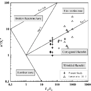
All flames can be considered to lie between the thin reaction zone and the corrugated flamelet zone, in the flamelet regime on the Peters-Borghi diagram (Borghi 1984, Peters 1988) in Fig. 3. 𝐾𝑎, the Karlovitz stretch number was calculated with the following expression 𝐾𝑎 = (𝛿𝐿⁄𝐿𝑇)1/2(𝑢′/𝑆𝐿0)3/2
with 𝐿𝑇 the integral length scale and 𝛿𝐿 the laminar flame thickness. 𝑀𝑎𝑏 was determined by dividing
the experimental 𝐿𝑏 by the laminar flame thickness, 𝛿𝐿, calculated as 𝐷𝑡ℎ/𝜌𝑢𝑐𝑝𝑆𝐿0 with 𝐷𝑡ℎ the thermal
calculated as 𝑙𝑛(𝜌𝑢/𝜌𝑏)/4 (Lipatnikov and Chomiak 2007) (with 𝜌𝑏 the burnt gas density) to
parametrize the large-scalestretching of turbulent flames (Bradley et al. 2011b). Finally the Damkohler number was obtained using the expression (𝐿𝑇⁄ ) ∗ (𝑢′ 𝑆𝛿𝐿 ⁄ 𝐿0). Isooctane-air mixtures were already
studied in (Lawes et al. 2012) and can be compared with the present work. Lawes et al. carried out their experiments with a lower temperature (360 K) in conditions of pressure similar to the present work: mainly 0.5 MPa (with a few additional tests at 0.1 and 1 MPa), equivalence ratio from 0.8 to 1.4 and turbulence intensities of 0.5, 1, 2, 4 and 6 m/s. The present work extend the database first at 0.1 MPa, second with more turbulent intensities ranging from 0.5 to 2.7 m/s and last with a lower integral length scale: 3.4 mm for the present study vs. 20 mm for (Lawes et al. 2012). The integral length scale of the present vessel is therefore closer to those observed in automotive Spark-Ignition engine, i.e. about 1.4 mm in (Mounaïm-Rousselle et al. 2013). For the sake of comparison the data of Lawes et al. at 0.1 and 0.5 MPa, equivalence ratio from 0.8 to 1.4 and all turbulence intensities were reported in the Peters-Borghi diagram in Fig. 3.
Table 1 – Turbulent and flame parameters for all investigated conditions. (* indicates that 7.5% of the total mixture is synthetic EGR dilutant).
𝑃0 (MPa) 𝛷 𝑢’ (m/s) 𝑅𝑒𝑇 𝑆𝐿0 (cm/s) 𝐿𝑏 (mm) 𝐿𝑒𝑒𝑓𝑓 𝛿𝐿 (µm) 𝑢’/𝑆𝐿0 𝐿𝑇/𝛿𝐿 𝐾𝑎 𝐷𝑎 𝑀𝑎𝑏 𝑀𝑎𝑡 0.1 0.8 0.52 65 39.2 1.1 2.52 95 1.33 35.8 0.256 26.92 11.58 0.42 0.1 0.8 1.04 131 39.2 1.1 2.52 95 2.65 35.8 0.721 13.51 11.58 0.42 0.1 0.8 1.39 173 39.2 1.1 2.52 95 3.55 35.8 1.118 10.08 11.58 0.42 0.1 1 0.52 66 53.6 0.78 1.98 67.8 0.97 50.1 0.135 51.65 11.50 0.44 0.1 1 0.69 88 53.6 0.78 1.98 67.8 1.29 50.1 0.207 38.84 11.50 0.44 0.1 1 1.04 131 53.6 0.78 1.98 67.8 1.94 50.1 0.382 25.82 11.50 0.44 0.1 1 1.39 177 53.6 0.78 1.98 67.8 2.59 50.1 0.589 19.34 11.50 0.44 0.1 1 1.73 219 53.6 0.78 1.98 67.8 3.23 50.1 0.820 15.51 11.50 0.44 0.1 1 2.08 264 53.6 0.78 1.98 67.8 3.88 50.1 1.079 12.91 11.50 0.44 0.1 1 2.43 308 53.6 0.78 1.98 67.8 4.53 50.1 1.362 11.06 11.50 0.44 0.1 1* 0.52 66 39.4 1 2 93 1.32 36.6 0.251 27.73 10.75 0.43 0.1 1* 1.04 131 39.4 1 2 93 2.64 36.6 0.709 13.86 10.75 0.43 0.1 1* 1.39 173 39.4 1 2 93 3.53 36.6 1.097 10.37 10.75 0.43 0.1 1.46 0.52 69 39.2 - 1.3 88 1.33 38.6 0.247 29.02 - 0.44 0.1 1.46 1.04 138 39.2 - 1.3 88 2.65 38.6 0.694 14.57 - 0.44 0.3 1 1.39 534 42.9 0.36 1.98 28.3 3.24 120.1 0.532 37.07 12.72 0.45 0.5 0.8 0.52 325 28.3 0.34 2.52 26 1.84 130.8 0.218 71.09 13.08 0.42 0.5 0.8 1.04 641 28.3 0.34 2.52 26 3.67 130.8 0.615 35.64 13.08 0.42 0.5 1* 0.52 334 28.4 0.27 2 26 1.83 130.8 0.216 71.48 10.38 0.43 0.5 1* 1.04 667 28.4 0.27 2 26 3.66 130.8 0.612 35.74 10.38 0.43 0.5 1 1.39 896 38.7 0.25 1.98 18.8 3.59 180.9 0.506 50.39 13.30 0.45 1 1 1.39 1804 33.6 0.15 1.98 10.8 4.14 314.8 0.475 76.04 13.89 0.45
Figure 3 – Peters-Borghi diagram for all conditions investigated.
Results and discussion
b. Determination of turbulent flame speed
Schlieren and tomographic images were post-processed using Matlab software to extract the flame contour as can be seen in Figure 2. All radii are given with an uncertainty of +/- 0.2 mm at 1 bar and +/- 0.5 mm at 5 bar.
Bradley et al. (Bradley et al. 2003) defined a reference radius 𝑅𝑣, such that the burnt gas volume
outside the sphere of this radius is equal to the unburnt gas volume inside it, to estimate the turbulent burning velocity from a planar flame sheet. 𝑅𝑣 corresponds to the radius from a contour at the mean
progress variable, 𝑐̃ = 0.5. It is a key parameter, since for the spherical surface defined by it: - the mass turbulent burning velocity and entrainment turbulent burning velocity are equal - the turbulent flame propagation speed is equal to the turbulent burning velocity multiplied
by the density ratio.
On the other hand, as the Schlieren flame contour contains both burned and unburned gases, the radius calculated from it, 𝑅𝑆𝑐ℎ, is not equal to 𝑅𝑣. Bradley et al. suggested the following empirical linear
equation:
𝑅𝑣 = 𝐶. 𝑅𝑆𝑐ℎ+ 𝐵 (1)
With 𝐶 and 𝐵, constant coefficients experimentally determined and suggested as 0.9 and -2.1 respectively by Bradley et al. (Bradley et al. 2003).
As the turbulent burning velocity can be estimated by 𝑈𝑡= 𝜌𝑏
𝜌𝑢.
𝑑𝑅𝑣
𝑑𝑡 with 𝜌𝑢 and 𝜌𝑏 respectively the
unburnt and burnt gas density, it can be written : 𝑈𝑡 = 𝜌𝑏 𝜌𝑢. 𝐶. 𝑑𝑅𝑆𝑐ℎ 𝑑𝑡 = 𝜌𝑏 𝜌𝑢𝐶. 𝑆𝑆𝑐ℎ (2)
with SSch, the turbulent propagation flame speed estimated from Schlieren technique and 𝐶 the constant
introduced in Eq. (1).
Since the flame is considered spherical, 𝑅𝑆𝑐ℎ = √𝐴𝑆𝑐ℎ/𝜋 and 𝑅𝑇𝑜𝑚𝑜 = √𝐴𝑇𝑜𝑚𝑜/𝜋 are respectively
the flame radii determined from Schlieren and tomographic images based on the burnt gas surface, A (Sch and Tomo respectively). The reference radius, 𝑅𝑣 is considered to be equal to 𝑅𝑇𝑜𝑚𝑜. As a
2-View Schlieren technique was set up, another radius was also estimated, based on the estimate of the flame volume: 𝑅𝑉,𝑆𝑐ℎ = (3𝑉𝑆⁄4𝜋)1/3. As shown in Fig. 2, from the side and front view Schlieren
images, the flame volume was determined by integrating the surface of the ellipses as a function of the z direction. These ellipses, indicated in grey in Figure 2, were fitted through four points defined from the two Schlieren contour projections.
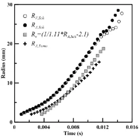
An example is given in Figure 4, where the average values of 𝑅𝑆𝑐ℎ, 𝑅𝑉,𝑆𝑐ℎ and 𝑅𝑇𝑜𝑚𝑜 are plotted
versus time for a stoichiometric mixture. First, as expected, no difference is distinguishable between the radius obtained from 2-View or 1-View Schlieren imaging, which confirms the sphericity of the flames and shows that the 1-View Schlieren technique is sufficient. Second, for all examples, 𝑅𝑇𝑜𝑚𝑜
are smaller than 𝑅𝑆𝑐ℎ, due to the 2D cut for the tomography and the 3D projection for Schlieren images.
The reference radius, 𝑅𝑣, estimated from Eq.1 by using the constant values of Bradley et al. is added.
In the first part of the flame development, 𝑅𝑣 is smaller than 𝑅𝑇𝑜𝑚𝑜 until 6ms. Then, from 6 to 9ms
the two radii display similar values before 𝑅𝑣 becomes greater than 𝑅𝑇𝑜𝑚𝑜. The constant values
determined by Bradley et al. were established for a set of 37 propane-air flame tests by considering flame radii between 2 and 40 mm. Since the experimental conditions in the present work are comparable to those investigated in (Bradley et al. 2003), the discrepancies observed between 𝑅𝑣 and
𝑅𝑇𝑜𝑚𝑜 could be due to the difference in radius range (less than 30 mm) or the fuel itself, which affects
the flame front wrinkling response to turbulence.
Figure 4 –Temporal evolution of different average radii at 𝑷𝟎= 0.1 MPa, 𝝓 = 1, T=423K, u’=1.04 m/s.
Hence, the constant C, also called the correction factor, was recalculated for the conditions (shaded in grey in Table 1) as
𝐶 = ⟨𝑑𝑅̅̅̅̅̅̅̅̅̅̅̅̅𝐴,𝑇𝑜𝑚𝑜
𝑑𝑅̅̅̅̅̅̅̅̅̅𝐴,𝑆𝑐ℎ ⟩𝑝𝑟𝑜𝑝𝑎𝑔𝑎𝑡𝑖𝑜𝑛 𝑑𝑢𝑟𝑎𝑡𝑖𝑜𝑛 𝑡𝑖𝑚𝑒 (3)
It should be mentioned that the 2-View Schlieren technique was only used to verify to what extent the flame can be considered spherical and also the effect of spark electrodes on its development. As shown in Fig. 4, for one example, the radius determined by the 2-View (𝑅𝑉,𝑆𝑐ℎ) or 1-View (𝑅𝑆𝑐ℎ) Schlieren
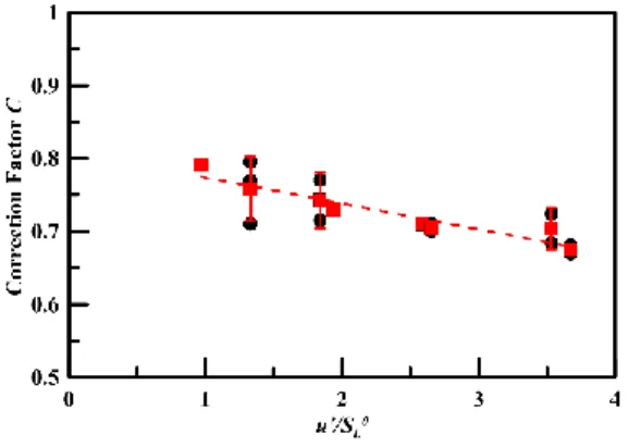
set-up was similar, with less than 3% difference. Therefore, in this study, only 1-View Schlieren imaging was used. For the other conditions only the 1-View Schlieren technique was used. For all conditions, between 8 and 10 tests were performed to provide sufficient data to ensure accuracy of the average. The variations on the flame speed were less than 5% and were not related to the pressure. All the values obtained for the correction factor were between 0.65 and 0.8, i.e. below 0.9 (Bradley et
al. 2003), as can be seen in Figure 5. These values are in a good agreement with a more recent study
by Bradley et al. (Bradley et al., 2011) where the values of the ratio 𝑅𝑣/𝑅𝑠𝑐ℎ (as defined at the
length scale in the ‘Leeds’ vessel is higher than the one of the present vessel (20 mm vs 3.4 mm). As a result, the integral length scale seems to be not so impacting for the correction factor 𝐶. However the correction factor appears to decrease with the increase in 𝑢’/𝑆𝐿0 . The trend seems to be valid because
if one considers the values at 𝑢’/𝑆𝐿0 = 1.33, the lowest average value for C is 0.72 which remains higher
than the lowest average value for C, i.e. 0.675, obtained at 𝑢’/𝑆𝐿0 =3.67. One explanation for this
decrease may be related to the impact of flame wrinkling. Since the Schlieren technique does not take wrinkles into account, the more wrinkled the flame is, the more differences are expected between the flame contours obtained from tomography and those from Schlieren techniques. As a result, since 𝑢’/𝑆𝐿0 is assumed from the data to be the parameter with the most impact, an empirical linear
correlation is suggested, namely 𝐶 = 𝑎 ∗𝑢′
𝑆𝐿0+ 𝑏 , where 𝑎 = −3.55.10
−2and 𝑏 = 0.81.
Figure 5 – Correction factor C as a function of 𝒖’/𝑺𝑳𝟎 for all data shaded in Table 1
Future investigations are required to evaluate it for 0<𝑢’/𝑆𝐿0< 1 as in laminar conditions the correction
factor has to be equal to 1.
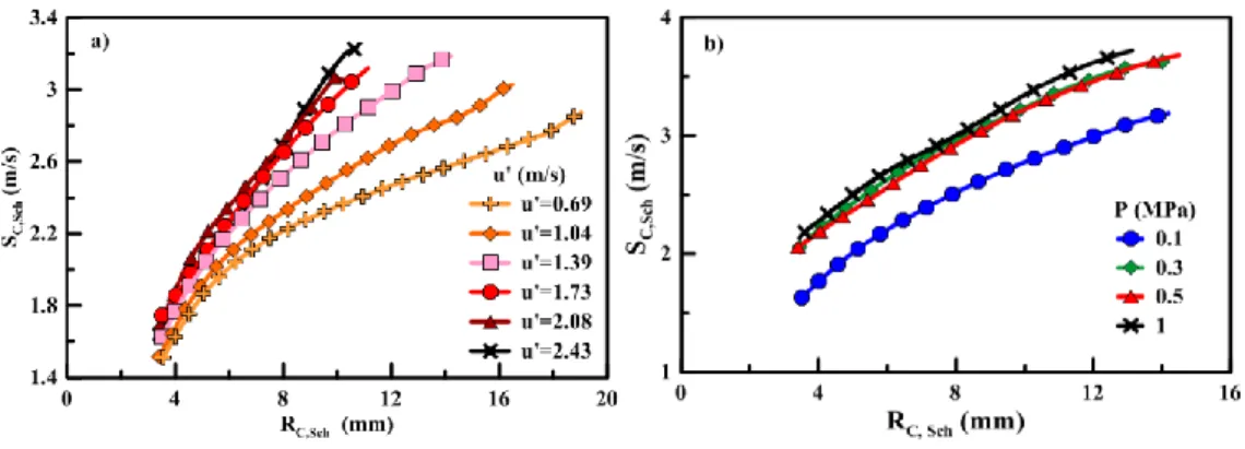
In Fig.6a and b, the evolution of 𝑆𝐶,𝑆𝑐ℎ, the turbulent flame speed obtained from Schlieren radii,
corrected by C, is plotted versus the corrected Schlieren radius for different turbulent intensities and different initial pressure conditions, respectively. As highlighted by Wu et al.(Wu et al. 2015) and Goulier et al.(Goulier et al. 2017), a typical property of turbulent expanding flames is the increase in the flame speed with the radius itself, mainly due to the increase in wrinkling. According to Bradley et al. (Bradley et al. 2011b) and Lawes et al. (Lawes et al. 2012), the flame can normally only be wrinkled by smaller sized eddies than itself and continues to increase until the flame kernel
encompasses the entire turbulence spectrum. Therefore, the flame speed has to reach a plateau at some point. Unfortunately, due to the size of the windows (70 mm diameter) and of the HIT zone (40 mm diameter) inside the spherical vessel, it is not possible to observe flame radii greater than 20 mm in most cases. However, even for a spherical vessel with a larger diameter, no experimental data obtained by Lawes et al. (Lawes et al. 2012), Goulier et al. (Goulier et al. 2017), Wu et al. (Wu et al. 2015) reached this condition.
Figure 6 –Flame propagation speed versus flame radius for different turbulent intensities (a) (𝑷𝟎=0.1 MPa) and different initial pressures (b) (u’=1.39 m/s), obtained from corrected Schlieren data. T=423 K, 𝜱 = 𝟏. 𝟎.
The increase in the turbulent flame speed due the turbulent intensity and pressure increases is due to the increase in the wrinkling. The effect of pressure for a “low” turbulent intensity is in good agreement with recent data by Lawes et al. (Lawes et al. 2012) done at u’=1m/s. In fact, as Galmiche et al.(Galmiche et al. 2013) showed, the increase in initial pressure in the vessel induces a decrease in the small turbulent length scales (i.e. Taylor and Kolmogorov ones), especially between 0.1 and 0.5 MPa. After 0.5 MPa, the small length scales cease to evolve for pressures higher than 0.5 MPa, which may explain the absence of effect on the flame speed. Moreover, as the flame thickness decreases with the pressure, the turbulent scale spectrum that can wrinkle the flame towards the small length scales is enlarged, increasing the wrinkles and therefore the flame speed. In fact, it can be seen that the evolution of 𝑆𝐶,𝑆𝑐ℎ is similar versus 𝑢’, when 𝑢’ ≥1.73 m/s and versus 𝑃0, when 𝑃0 ≥ 0.3 MPa, which
concerning the determination of the turbulent burning velocity (Lawes et al. 2012, Wu et al. 2015, Goulier et al. 2017).
b. Effect of global stretch
Because a propagating flame surface undergoes global curvature, local curvature and flow field strain, the total stretch 𝜅 quantifying the turbulence-flame interaction can be separated into 3 terms according to (Chaudhuri et al. 2015) : 𝜅 = 𝑆⏟𝐿𝜅 𝑠𝑡𝑟𝑒𝑡𝑐ℎ 𝑟𝑎𝑡𝑒 𝑏𝑦 𝑐𝑢𝑟𝑣𝑎𝑡𝑢𝑟𝑒: 𝜅𝑐,𝑅 − (v.n)𝜅⏟ 𝑛𝑜𝑟𝑚𝑎𝑙 𝑠𝑡𝑟𝑎𝑖𝑛 𝑟𝑎𝑡𝑒: 𝜅𝑛 ⏞ 𝑠𝑡𝑟𝑒𝑡𝑐ℎ 𝑟𝑎𝑡𝑒 𝑏𝑦 𝑐𝑢𝑟𝑣𝑎𝑡𝑢𝑟𝑒: 𝜅𝜅 + ∇⏟𝑡. vt 𝑡𝑎𝑛𝑔𝑒𝑛𝑡𝑖𝑎𝑙 𝑠𝑡𝑟𝑎𝑖𝑛 𝑟𝑎𝑡𝑒: 𝜅𝑡 (4)
This is also similar to the previous work by Candel and Poinsot (Candel and Poinsot 1990).
The first term represents the stretch due to curvature, 𝜅𝑐,𝑅, and the second and third ones the stretch
rate contributions by the strain rate, 𝜅𝑠. 𝜅𝑐,𝑅 is the sum of the stretch rate due to local wrinkling and
the strain rate due to the global flame shape. For a spherical propagation, it is calculated as: 𝜅𝑐,𝑅 = 2
𝑅𝑆𝑐ℎ
𝑑𝑅𝑆𝑐ℎ
𝑑𝑡 (5)
As isooctane is more sensitive to stretch than methane (Brequigny, Halter, Mounaïm-Rousselle, et al. 2016), the global and local stretches will delay the flame speed increase during propagation (Bradley
et al. 2011b, Brequigny, Halter, and Rousselle 2016, Brequigny, Halter,
Mounaïm-Rousselle, et al. 2016), especially for small radii. In Fig.7, the corrected turbulent flame speed estimated from Schlieren images 𝑆𝐶,𝑆𝑐ℎ is plotted versus 𝜅𝑐,𝑅. As the flame radius during the first part
of propagation in the case of spherical propagation is small, it generates strong curvature. This curvature tends to decrease rapidly with the increase in the flame radius. The nonlinear extrapolation of laminar propagation speed evolution, obtained in the same conditions (Endouard et al. 2016) is also plotted. From Figure 7, similarities can be observed between the development of turbulent and laminar flame speeds as a function of stretch: first, the flame speed decreases due to the ignition effect, then the flame speed increases as flame stretch decreases and then exceeds the laminar curve especially for 𝑢’ >1.04 m/s. Moreover after the ignition effects disappear, in the early stage of flame development, the values of flame speed and flame stretch obtained for turbulent cases are comparable to those of the
laminar cases. The main effect of the correction of the Schlieren images is to improve the agreement with the nonlinear laminar extrapolation model. Good agreement was found with Lipatnikov and Chomiak (Lipatnikov and Chomiak 2007), who used Bradley et al.'s data to analyze the effect of global stretch on the burning turbulent velocity. By analogy with the classical Markstein number, they defined a turbulent Markstein number, 𝑀𝑎𝑡, to characterize the burning turbulent velocity variations, not as a
function of the local stretch rate but of the global one. As can be seen in Table 1, 𝑀𝑎𝑡 is in the same
order for all conditions. This means that for all turbulent intensities, the flame propagation speed follows globally the laminar development before being impacted by turbulence and exceeding the laminar curve especially for 𝑢’ >1.04 m/s. By analogy with the laminar speed evolution, 𝑈𝑡0, the value
of 𝑈𝑡 from the interpolation to 𝜅𝑐,𝑅= 0 can be determined (Lipatnikov and Chomiak 2007, Brequigny,
Halter, Mounaïm-Rousselle, et al. 2016).
Figure 7– Turbulent flame speed versus the global stretch for different turbulent intensities based on corrected Schlieren data. Continuous line: nonlinear extrapolation model for laminar propagation in the same initial conditions.
𝑷𝟎=0.1 MPa, T=423 K, 𝜱=1.0.
c. Estimate of turbulent burning velocity
As previously discussed, spherical expanding turbulent flames continuously accelerate and an asymptotic value, which corresponds to absolute values of 𝑈𝑡, cannot be determined in the case of
most expanding flames. Wu et al. (Wu et al. 2015) suggested the following average turbulent burning velocity definition:
𝑈𝑡,𝑚𝑒𝑎𝑛 = 𝜌𝑏 𝜌𝑢. 3 ∫𝑅2〈𝑅〉2(𝑑〈𝑅〉⁄𝑑𝑡)𝑑〈𝑅〉 𝑅1 〈𝑅2〉3−〈𝑅 1〉3 (6) where 𝑅1 and 𝑅2 are 10 and 20 mm, respectively.
From Lipatnikov and Chomiak (Lipatnikov and Chomiak 2007), the extrapolation of the evolution of
𝑈𝑡 versus the global stretch at zero stretch should provide a more universal value, 𝑈𝑡 (𝜅𝑐,𝑅= 0). In
Fig.8 and 9, these different estimates of 𝑈𝑡, normalized by the unstretched laminar flame velocity
𝑆𝐿0 are plotted versus the usual ratio 𝑢′/𝑆
𝐿0, for all data conditions at 𝑃0 = 0.1 and 0.5 MPa respectively.
In (Lawes et al. 2012), Lawes et al. choose their last measurable data at R=30 mm. The values of Lawes et al. have been added for the conditions closest to those of Table 1. By analogy, the 𝑈𝑡 values
reached at R=20 mm in the present study can also be considered.
First, as expected, the lowest estimate of the turbulent burning velocity is obtained by 𝑈𝑡 (R=20 mm),
as the turbulent flame propagation velocity does not reach a plateau at this radius. The estimates of 𝑈𝑡 from Eq.6 are the highest ones. Indeed, due to its definition itself, 𝑈𝑡,𝑚𝑒𝑎𝑛 is calculated for radii
between 10 and 20 mm whereas 𝑈𝑡 (𝜅𝑐,𝑅= 0) is obtained from the extrapolation on the longest linear
part. The best radius range for the linear extrapolation starts for radius a little bit higher than 4 mm as shown in Fig. 7. Globally a good agreement with the data from Lawes et al. is obtained for 𝑈𝑡 (𝜅𝑐,𝑅=
0) at both initial pressures. For comparison, various correlations of turbulent burning velocity are
presented in Fig. 8 and 9. Fist the correlation of (Kobayashi et al. 1998), defined in Eq. 7 is introduced.
𝑈𝑡 𝑆𝐿0 = 𝐴𝑘[( 𝑃 𝑃𝑟𝑒𝑓) ( 𝑢′ 𝑆𝐿0)] 0.4 (7) with 𝐴𝑘 a constant originally set to 1.9.
In Fig. 8 and 9, three other estimates of 𝑈𝑡/𝑆𝐿0 were also added:
- the first one (dashed line) suggested by Lawes et al.(Lawes et al. 2012) according to the dataset of Bradley et al. (Bradley et al. 1992), based on 𝐾𝑎. 𝐿𝑒 values to take into account the effect of thermal diffusivity/strain.
𝑈𝑡
𝑆𝐿0 = 𝐴𝑏. 𝑢′
𝑆𝐿0(𝐾𝑎𝐿𝑒)
with 𝐴𝑏 a constant, estimated equal to 0.88 from the dataset of Bradley et al.
- the second one (dotted line) suggested by Zimont (Lipatnikov and Chomiak 2002), with the form developed by Driscoll (Driscoll 2008):
𝑈𝑡 𝑆𝐿0 = 1 + 𝐴𝑧( 𝑢′ 𝑆𝐿0) 0.5 𝑅𝑒𝑇0.25 (9)
with 𝐴𝑧 a constant originally equal to 0.4 as suggested by (Lawes et al. 2012).
- The last one (dashed dotted line) came from another form of Zimont but by integrating the Lewis Number and Pressure provided by (Muppala et al. 2005):
𝑈𝑡 𝑆𝐿0= 1 + 𝐴𝑚 𝐿𝑒𝑒𝑓𝑓𝑅𝑒𝑇 0.25(𝑢′ 𝑆𝐿0) 0.3 ( 𝑃 𝑃𝑟𝑒𝑓) 0,2 (10)
with 𝐴𝑚 a constant originally equal to 0.46.
It can be noted that the estimates from Eq. 7, 8, and 9 predict higher values than the experiments using the ‘original’ pre-estimated constant values (black lines in Fig.8 and 9). However, the estimates from Eq.10 are in very good agreement with the experimental estimate 𝑈𝑡,𝑚𝑒𝑎𝑛 for both initial pressures
even with the original constant determined by (Muppala et al. 2005). The correlation of Kobayashi et al. highly overestimates the 3 experimental estimates of 𝑈𝑡. This can be explained by the fact that the
correlation of Kobayashi et al. was obtained from the assumption of the development of flame in a fully turbulent regime, which is not the case in the present vessel. According to (Bradley et al. 2011a) this happens when the flame radius is higher than 8 times 𝐿𝑇 (so higher than 27 mm). One possible
way to improve the results would be to use the effective rms turbulent velocity 𝑢𝑘′ which correspond
to the turbulence actually seen by the flame front, smaller than 𝑢′ (Bradley et al. 2011b, Mannaa et al.
2018). The discussion is similar for the overestimate of Eq. (8) which should be computed using 𝑢𝑘′
instead of 𝑢′. Moreover, the correlation of Kobayashi et al. was determined with propane as fuel, so to evaluate it with isooctane implies a modification of the constant 𝐴𝑘 and of the exponent factor. The
modification of the value of 𝐴𝑘 compared with the value of Kobayashi et al. is due to the change of
number. In conclusion, the reason for the overestimation of the Kobayashi correlation may be twofold: the fact that the actual turbulence has not been taken into account and the underestimation of the Lewis number effect. Last, the better agreement with 𝑈𝑡,𝑚𝑒𝑎𝑛 and trend obtained with the correlation of
Muppala et al. could be explained by the fact that its correlation takes into account most of the combustion parameters i.e. the Lewis number, the length scale through the Reynolds, the turbulent intensity, the chemistry through 𝑆𝐿0, and the pressure.
Figure 8 – Comparison of various correlations for 𝑼𝒕/𝑺𝑳𝟎 as a function of 𝒖′/𝑺𝑳𝟎 versus experimental data at 𝑷𝟎=0.1 MPa
Figure 9 – Comparison of various correlations for 𝑼𝒕/𝑺𝑳𝟎 as a function of 𝒖′/𝑺𝑳𝟎 versus experimental data at 𝑷𝟎=0.5 MPa
(black lines: original correlation, grey lines: adapted correlation).
In order to adapt the predicted estimates to our dataset, the constants 𝐴𝑏, 𝐴𝑧, 𝐴𝑘, 𝐴𝑚 in Eq. 7, 8, 9 and
10 were optimized to 0.36, 0.06, 0.95 and 0.2 respectively as done previously (Burke et al. 2016). These predicted estimates are plotted in Fig. 8 and 9 in grey. The optimizations were done by minimizing the differences between the predicted and experimental data from this study 𝑈𝑡 (𝜅𝑐,𝑅= 0)
and from Lawes et al. but only by considering 𝑃0 = 0.1 MPa data. In order to evaluate the performance
of the modified correlations, the mean average absolute differences with the experimental data calculated as follows are summarized in Table 2:
Δ𝑈𝑡 𝑈𝑡 (%) ̅̅̅̅̅̅̅̅̅ = ∑ 𝑎𝑏𝑠(𝑈𝑡,𝑐𝑜𝑟𝑟𝑒𝑙𝑎𝑡𝑖𝑜𝑛−𝑈𝑡,𝑒𝑥𝑝(𝜅𝑐,𝑅=0)) 𝑈𝑡,𝑒𝑥𝑝(𝜅𝑐,𝑅=0) ∗100 𝑛 𝑖=1 𝑛 (11)
Table 2 – Mean absolute percentage difference with the modified correlations described in Eq. 7, 8, 9 and 10 for 0.1 and 0.5 MPa. 𝑃0 (MPa) (Δ𝑈𝑡 𝑈𝑡 ) ̅̅̅̅̅̅̅̅ 𝐵𝑟𝑎𝑑𝑙𝑒𝑦 (𝐸𝑞.8) (Δ𝑈𝑡 𝑈𝑡 ) ̅̅̅̅̅̅̅̅ 𝑀𝑢𝑝𝑝𝑎𝑙𝑎 (𝐸𝑞.10) (Δ𝑈𝑡 𝑈𝑡 ) ̅̅̅̅̅̅̅̅ 𝑍𝑖𝑚𝑜𝑛𝑡 (𝐸𝑞.9) (Δ𝑈𝑡 𝑈𝑡 ) ̅̅̅̅̅̅̅̅ 𝐾𝑜𝑏𝑎𝑦𝑎𝑠ℎ𝑖 (𝐸𝑞.7) 0.1 9.8 14.2 11.1 7.4 0.5 12.1 8.2 20.9 44.0
The optimized estimates from Bradley et al. and Muppala et al. are globally in good agreement even at higher pressure. These two correlations take into account both thermochemical properties (with the Lewis number) and flame turbulence interaction (with either the Karlovitz stretch number or the turbulent Reynolds number). Contrary to what was expected, the effect of pressure on the turbulent burning velocity is not well captured by the ‘optimized’ correlation of Kobayashi et al., even if it based on the pressure effect. Finally, the optimized estimate from Zimont et al. displays quite acceptable values but from Fig. 8 and 9 it appears that this correlation performs less well at high turbulence levels (𝑢′/𝑆
Conclusion
In this paper, the empirical correlation between different flame radii (obtained from Mie scattering and Schlieren techniques) suggested by Bradley et al. (Bradley et al. 2003) was assessed in order to ensure the validity of the turbulent propagation flame speed estimate from Schlieren images in the case of an iso-octane/air mixture. The correction factor was found to be dependent on turbulence and flame properties, i.e. 𝑢’/𝑆𝐿0 and displayed values globally in agreement with a more recent study
by Bradley et al. (Bradley et al. 2011a). However, further work on lower turbulent intensities, higher pressures and dilution rates is still needed to improve this correlation.
The influence of turbulent intensity and pressure was investigated in terms of turbulent flame propagation speed as a function of radius and global stretch to better understand the dynamic of flame propagation. Different estimates of turbulent burning velocities from the experimental data were compared to evaluate their robustness to provide accurate data, comparable to those obtained from different flame configurations to improve model development. Finally, they were compared to estimates from different correlations in the literature to improve the consistency of the experimental data and of these correlations. It was found that the estimates from Muppala et al.’s correlation (Muppala et al. 2005) satisfactorily reproduced the experimental values obtained from the definition introduced by Wu et al. (Wu et al. 2015). The other correlations overestimated the experimental data from this study and those provided by Lawes et al. In conclusion, the turbulent burning velocity obtained from extrapolation of burning velocity at zero stretch appears to be a good estimate, in good agreement with the ‘optimized’ estimates from Bradley et al. and the correlation by Muppala et al., where thermochemical properties and turbulence-flame interaction were taken into account.
Acknowledgements
This work was financed by the MACDOC project from the French National Research Agency, ANR-12-VPTT-0008.
References
Aleiferis, P.G., Serras-Pereira, J., and Richardson, D., 2013. Characterisation of flame development with ethanol, butanol, iso-octane, gasoline and methane in a direct-injection spark-ignition engine. Fuel, 109, 256–278.
Bagdanavicius, A., Bowen, P.J., Bradley, D., Lawes, M., and Mansour, M.S., 2015. Stretch rate effects and flame surface densities in premixed turbulent combustion up to 1.25 MPa.
Combustion and Flame, 162 (11), 4158–4166.
Bechtold, J.K. and Matalon, M., 2001. The dependence of the Markstein length on stoichiometry.
Combustion and Flame, 127 (1–2), 1906–1913.
Borghi, R., 1984. Mise au point sur la structure des flammes turbulentes. Journal de chimie
physique, 81 (6), 361–370.
Bradley, D., Haq, M.Z., Hicks, R.A., Kitagawa, T., Lawes, M., Sheppard, C.G.W., and Woolley, R., 2003. Turbulent burning velocity, burned gas distribution, and associated flame surface
definition. Combustion and Flame, 133 (4), 415–430.
Bradley, D., Lau, A.K.C., and Lawes, M., 1992. Flame Stretch Rate as a Determinant of Turbulent Burning Velocity. Philosophical Transactions of the Royal Society of London. Series A:
Physical and Engineering Sciences, 338 (1650), 359–387.
Bradley, D., Lawes, M., and Mansour, M.S., 2011a. Correlation of turbulent burning velocities of ethanol–air, measured in a fan-stirred bomb up to 1.2MPa. Combustion and Flame, 158 (1), 123–138.
Bradley, D., Lawes, M., and Mansour, M.S., 2011b. The problems of the turbulent burning velocity.
Flow, Turbulence and Combustion, 87 (2–3), 191–204.
Brequigny, P., Halter, F., and Mounaïm-Rousselle, C., 2016. Lewis number and Markstein length effects on turbulent expanding flames in a spherical vessel. Experimental Thermal and Fluid
Science, 73, 33–41.
Brequigny, P., Halter, F., Mounaïm-Rousselle, C., and Dubois, T., 2016. Fuel performances in Spark-Ignition (SI) engines: Impact of flame stretch. Combustion and Flame, 166, 98–112.
Burke, E.M., Güthe, F., and Monaghan, R.F.D., 2016. A Comparison of Turbulent Flame Speed Correlations for Hydrocarbon Fuels at Elevated Pressures. In: ASME Turbo Expo 2016:
Turbomachinery Technical Conference and Exposition. V04BT04A043.
Candel, S.M. and Poinsot, T.J., 1990. Flame Stretch and the Balance Equation for the Flame Area.
Combustion Science and Technology, 70 (1–3), 1–15.
Chaudhuri, S., Saha, A., and Law, C.K., 2015. On flame–turbulence interaction in constant-pressure expanding flames. Proceedings of the Combustion Institute, 35 (2), 1331–1339.
Chaudhuri, S., Wu, F., Zhu, D., and Law, C.K., 2012. Flame speed ans self similar propagation of expanding turbulent premixed flames. Physical review Letters, 108 (044503).
Driscoll, J.F., 2008. Turbulent premixed combustion: Flamelet structure and its effect on turbulent burning velocities. Progress in Energy and Combustion Science, 34 (1), 91–134.
Endouard, C., Halter, F., Chauveau, C., and Foucher, F., 2016. Effects of CO 2 , H 2 O, and Exhaust
Gas Recirculation Dilution on Laminar Burning Velocities and Markstein Lengths of Iso-Octane/Air Mixtures. Combustion Science and Technology, 188 (4–5), 516–528.
Galmiche, B., Halter, F., and Foucher, F., 2012. Effects of high pressure, high temperature and dilution on laminar burning velocities and Markstein lengths of iso-octane/air mixtures.
Combustion and Flame, 159 (11), 3286–3299.
Galmiche, B., Mazellier, N., Halter, F., and Foucher, F., 2013. Turbulence characterization of a high-pressure high-temperature fan-stirred combustion vessel using LDV, PIV and TR-PIV
measurements. Experiments in Fluids, 55 (1), 1–20.
Gillespie, L., Lawes, M., Sheppard, C.G.W., and Woolley, R., 2000. Aspects of Laminar and Turbulent Burning Velocity Relevant to SI Engines. SAE Technical Paper, (2001-1–192). Goulier, J., Comandini, A., Halter, F., and Chaumeix, N., 2017. Experimental study on turbulent
expanding flames of lean hydrogen/air mixtures. Proceedings of the Combustion Institute, 36 (2), 2823–2832.
Kobayashi, H., Kawabata, Y., and Maruta, K., 1998. Experimental study on general correlation of turbulent burning velocity at high pressure. Symposium (International) on Combustion, 27 (1),
941–948.
Lawes, M., Ormsby, M.P., Sheppard, C.G.W., and Woolley, R., 2012. The turbulent burning velocity of iso-octane/air mixtures. Combustion and Flame, 159 (5), 1949–1959.
Lipatnikov, A. and Chomiak, J., 2007. Global stretch effects in premixed turbulent combustion.
Proceedings of the Combustion Institute, 31 (1), 1361–1368.
Lipatnikov, A.N. and Chomiak, J., 2002. Turbulent flame speed and thickness: phenomenology, evaluation, and application in multi-dimensional simulations. Progress in Energy and
Combustion Science, 28 (1), 1–74.
Mannaa, O., Brequigny, P., Mounaim-Rousselle, C., Foucher, F., Chung, S.H., and Roberts, W.L., 2018. Turbulent burning characteristics of FACE-C gasoline and TPRF blend associated with the same RON at elevated pressures. Experimental Thermal and Fluid Science, 95, 104–114. Matalon, M. and Creta, F., 2012. The "turbulent flame speed" of wrinkled premixed
flames. Comptes Rendus Mecanique, 340, 845–858.
Mounaïm-Rousselle, C., Landry, L., Halter, F., and Foucher, F., 2013. Experimental characteristics of turbulent premixed flame in a boosted Spark-Ignition engine. Proceedings of the Combustion
Institute, 34 (2), 2941–2949.
Muppala, S.P.R., Aluri, N.K., Dinkelacker, F., and Leipertz, A., 2005. Development of an algebraic reaction rate closure for the numerical calculation of turbulent premixed methane, ethylene, and propane/air flames for pressures up to 1.0 MPa. Combustion and Flame, 140 (4), 257–266. Peters, N., 1988. Laminar flamelet concepts in turbulent combustion. Symposium (International) on
Combustion, 21 (1), 1231–1250.
Renou, B. and Boukhalfa, A., 2001. An Experimental Study of Freely Propagating Premixed Flames at Various Lewis Numbers. Combustion Science and Technology, 162 (1), 347–370.
Verma, S. and Lipatnikov, A.N., 2016. Does sensitivity of measured scaling exponents for turbulent burning velocity to flame configuration prove lack of generality of notion of turbulent burning velocity? Combustion and Flame, 173, 77–88.
flames of C4 to C8 n-alkanes at elevated pressures: Experimental determination, fuel similarity, and stretch-affected local extinction. Proceedings of the Combustion Institute, 35 (2), 1501– 1508.
Figure Captions
Figure 1 – Experimental setup. L1 and L2 : LED, PM : parabolic mirror, C1 Phantom v1610 Camera, C2 Phantom v1210 Camera, FM Dot point, LE Lenses.
Figure 2 – Example of images. (a) front view Schlieren image, (b) side view Schlieren image, (c) Mie scattering image, side view, (d) reconstructed flame volume.
Figure 3 – Peters-Borghi diagram for all conditions investigated.
Figure 4 – Temporal evolution of different average radii at 𝑃0= 0.1 MPa, 𝜙 = 1, T=423K, 𝑢’=1.04 m/s.
Figure 5 – Correction factor as a function of 𝑢’/𝑆𝐿0 for all data shaded in grey in Table 1.
Figure 6 – Flame propagation speed versus flame radius for different turbulent intensities (a) (𝑷𝟎=0.1
MPa) and different initial pressures (b) (u’=1.39 m/s), obtained from corrected Schlieren data. T=423 K, 𝜱 = 𝟏. 𝟎.
Figure 7 – Turbulent flame speed versus the global stretch for different turbulent intensities based on corrected Schlieren data. Continuous line: nonlinear extrapolation model for laminar propagation at the same initial conditions. 𝑷𝟎=0.1 MPa, T=423 K, Φ=1.0.
Figure 8 – Comparison of various correlations for 𝑈𝑡/𝑆𝐿0 as a function of 𝑢′/𝑆𝐿0 versus experimental
data at 𝑃0=0.1 MPa (black lines: original correlation, grey lines: adapted correlation).
Figure 9 – Comparison of various correlations for 𝑈𝑡/𝑆𝐿0 as a function of 𝑢′/𝑆𝐿0 versus experimental
data at 𝑃0=0.5 MPa (black lines: original correlations, grey lines: adapted correlation).
Table 2 – Turbulent and flame parameters for all investigated conditions. (* indicates that 7.5% of the total mixture is synthetic EGR dilutant).
Table 2 – Mean absolute percentage difference with the modified correlations described in Eq. 7, 8, 9 and 10 for 0.1 and 0.5 MPa