Complexity cost quantification and modeling for strategic portfolio management

Complexity Cost Quantification and Modeling for Strategic Portfolio

By Jan Ma

B.S. Biological Environmental Engineering, Cornell University, 2007

Submitted to the MIT Sloan School of Management and the Mechanical Engineering Partial Fulfillment of the Requirements for the Degrees of

Master of Business Administration and

Master of Science in Mechanical Engineering

In conjunction with the Leaders for Global Operations Program at the Massachusetts Institute of Technology

June 2014

Department in

I

OF TECHNOLOGY

JUN

2014

LIBRARIES

The author hereby grants to MIT permission to reproduce and to distribute publicly paper and electronic copies of this thesis document in whole or in part in any medium now known or peafter.

Signature of Author

Signature redacted

Certified by

MIT Sloan School of Management, MIT Department of fianical Engineering May 9, 2014

Donald Rosenfield, Thesis Supervisor Senior Lecturer, MIT Sloan School of Management

Certified by

Signature redacted...

Josef Oehmen, Thesis Supervisor Associate Professor, Department of Management Engineering, Technical Universitif Den rk

C-etfdA b &.*A

Certified by

Signature red acted

St iley B. Gerfiwin, Thesis Reader Senior Research Scientist, D a t ent of ec icc Engineering

Signature redacted'

Accepted by

'

David E. Hardt, Chair Mechanical Engineeriny Committee on Graduate Students

Signature redacted

Accepted by

Vjaura Herson, Dirdctor, MBA Program MIT Sloan School of Management

Complexity Cost Quantification and Modeling for Strategic Portfolio Management

By Jan Ma

Submitted to the MIT Sloan School of Management and the MIT Department of Mechanical Engineering on May 9, 2014 in partial fulfillment of the requirements for the

Degrees of Master of Business Administration and Master of Science in Mechanical Engineering

Abstract

This project explores portfolio management and planning through effectively reducing complexity within operations. We apply this to a major healthcare company (referred to as Company X). The anticipated launch of new molecules and formulations into the existing high mix product portfolio presents significant challenges to contain cost and maintain the standard service level of Company X.

Complexity costs associated with manufacturing and supply chain activities are not entirely accounted for in direct production costs. Having transparency to these costs at a brand or SKU level would allow significant improvements in strategic decision making throughout the life cycle of a product. The work outlined in this thesis describes the development of a quantification model to capture operational complexity costs as well as an analysis of potential impact for Company X associated with implementation of the model. This is accomplished through first, identifying and prioritizing complexity cost generators; second, quantifying the costs through application of activity based

accounting; third, building and piloting a decision support tool and NPV model. Lastly, process for implementation and application of the model was defined.

The findings from this project provide financial rationale for a 27% reduction in the total product portfolio size, which results in a potential savings of $75M over the next five years, and 50% human resource savings across the Technical Operations and key support functions at Company X. The model can be a powerful tool for optimizing product portfolios with attention to financial, operational, and strategic considerations. Reducing complexity creates the ability to become more discerning about the portfolio composition and enable Company X to focus even more on high growth and life-saving brands. Thesis Supervisor: Donald Rosenfield

Title: Senior Lecturer, Operations Management, MIT Sloan School of Management Thesis Supervisor: Josef Oehmen

Title: Associate Professor, Management Engineering, Technical University of Denmark Thesis Reader: Stanley B. Gershwin

Acknowledgments

I would like to thank all the faculty and staff of the Leaders for Global Operations Program for their support and guidance during this internship and through the past two years.

I would like to thank the managers, sponsors, and colleagues at Company X for their insights, coaching, and advocacy during my time in Basel and through the completion of my thesis. Specifically, Beat Rutishauser for always making time for the 'important stuff' and Erich Battanta, Ute Kessel, and Mario Joseph for their mentorship. Thank you to my local friends who were patient enough to teach me the cultural norms and show me around town, which made my time in Switzerland so enjoyable.

Thank you to my advisors, Don Rosenfield and Josef Oehmen for providing invaluable oversight and feedback throughout the internship and preparation of this thesis. I learned immensely from your expertise, attention to detail, and wisdom.

Thank you to my awesome fellow classmates for all the advice and memories. Especially those in Europe, it wouldn't have been the same without you guys.

I am eternally grateful to my family and friends for being with me every step of the way, making the last two years an unforgettably amazing experience. Thanks mom for being my solid support, sounding board, and tireless cheerleader through the years. Thanks Tey for sticking by me on this incredible journey. You have kept me sane and grounded through all the low and high points; without your love, understanding, and support, none of this would have been possible.

Table of Contents

Abstract ... 3

Acknowledgm ents... 5

Table of Contents... 7

List of Figures... 8

1 Introduction to Pharmaceutical Industry and Focus Company... 11

1.1 Pharm aceutical Industry Background ... 11

1.2 Com pany X Background... 11

1.3 Challenges Facing Com pany X ... 12

1.4 Project Objective... 15

1.5 Hypothesis...16

1.6 Thesis Structure...16

2 Literature Review of Com plexity Cost M odeling ... 17

2.1 Defining Com plexity in An Organization... 17

2.2 Sum m ary of Previous Com plexity Reduction Projects... 20

2.3 Review of Methodologies Used in Complexity Cost Modeling... 21

3 Approach to Quantify and Model Complexity Costs... 24

3.1 Approach Sum m ary ... 24

3.2 Product Com plexity ... 25

3.2.1 Classification of Complexity Cost Generators ... 26

3.2.2 Data Gathering ... 27

3.2.3 Basic Structure of The Complexity Cost M odel... 29

3.2.4 Other Considerations for The M odel... 31

3.2.5 Incorporating Risk and Uncertainties into The M odel ... 31

3.2.6 Building The Net Present Value M odel... 33

3.2.7 Building the Decision Tree M odel ... 33

3.2.8 Data Validation ... 37

3.2.9 Key Assumptions ... 38

3.2.10 Using Case Studies to Validate M odel... 40

3.3 Process Com plexity... 41

3.4 Organizational Com plexity... 41

4 Results of M odel Application ... 42

4.1 General Findings ... 42

4.2 Case Study 1 - High Risk Category: Brand A ... 43

4.3 Case Study 2 - M edium Risk Category: Brand B... 45

4.4 Case Study 3 - Low Risk Category: Brand C ... 45

4.5 Process Com plexity Results ... 46

5 D iscussion & Next Steps ... 47

5.1 Shortcom ings and Lim itations of The M odel... 47

5.2 Further M odel Developm ent ... 48

5.3 Next Steps for Com pany X ... 48

5.3.2 A pplication of T he M odel...4 9

6 C onclusion ... 5 0

6.1 Summary of Work and Findings ... 50

6.2 Managerial Implications... 52

Appendix 1: Complexity Cost Measurement Metrics ... 55

Appendix 2: Model Inputs and Data Table ... 56

Appendix 3: Complexity Cost Model Outputs... 57

Appendix 4: Additional Results... 58

7 R eferences... ... ... 59

List of Figures Figure 1: Indirect operational costs that are not captured in accounting system of C o m p an y X ... 1 3 Figure 2: Product portfolio makeup of Company X... 13

Figure 3: Functional workload across Technical Operations over the lifecycle of a p ro d u ct...1 4 Figure 4: Average timeframe to complete execution of supply point decisions... 15

Figure 5: The three dimensions of complexity and associated examples of each [6]...18

Figure 6: Illustration of the complexity cube ... 19

Figure 7: General profitability curve of a product portfolio [6]... 20

Figure 8: Sample schematic of a typical MILP supply chain model [13]... 22

Figure 9: Indirect costs are displacing direct costs in integrated businesses [14]...23

Figure 10: Summary of thesis approach and project phases... 25

Figure 11: Identifying cost generating activities by functional involvement in supply p o in t actio n s ... 2 6 Figure 12: Classification of complexity cost generating tasks by impact and frequency of o ccurrence ... 2 7 Figure 13: Complexity cost model structure... 30

Figure 14: Decision Tree basic structure... 34

Figure 15: Skeleton of decision tree model... 36

Figure 16: Model validation schematic... 37

Figure 17: Breakdown of major complexity costs by category... 42

Figure 18: Portfolio effects of complexity reduction... 43

Figure 19: Five year gross margins forecast for Brand M ... 44

Figure 20: Five year gross margins forecast for Brand R... 46

Figure 21: Profitability whale curve [6]... 53

Figure 22: Complexity Cost as Percentage of Consolidated Total Production Cost...55

Figure 23: Relationship between Revenue and total SKUs for Brand M ... 55

Figure 24: Complexity Cost Model Main User Input... 56

Figure 26: Current and Ideal State Mapping Results for Lifecycle Management Decision M ak ing P ro cess... _{5 8} Figure 27: _{Sensitivity Analysis of Decision Tree Model ... 58}

1 Introduction to Pharmaceutical Industry and Focus Company

1.1 Pharmaceutical Industry Background

Pharmaceutical companies develop, manufacture, and market patented and generic therapeutics to treat a variety of illnesses. The sector is characterized by high barriers of entry but high rate of return. Lengthy and costly development lifecycles, competition through scale, and diversification of therapeutic targets are hallmarks of the industry. The pharmaceuticals industry has

traditionally been a very lucrative business, with a global market value of $300B a year [1]. However, in the recent decades, increasing Research and Development costs, competition from low cost generics, and regulatory pressures has slowly eroded the profitability of this business. Major pharmaceutical firms are continuously seeking means to operate more efficiently and sustain their cost advantages.

1.2 Company X Background

Company X is a leading global healthcare company headquartered in Basel, Switzerland. Company X has a diverse portfolio, including pharmaceuticals, eye care, consumer health products, and vaccines. Of all the product categories, pharmaceutical is the largest division, comprising 57% of net sales in 2012.

With operations in over 140 countries, the Technical Operations function manages a large and complex manufacturing and distributions network spread across 49 internal production sites and

280 contract manufacturers. In addition, a product portfolio mix of over 250 brands, totaling

overl5,000 SKUs makes supply point decisions particularly challenging.

Company X is an industry leader in innovations and has a robust pipeline with 15 new molecules slated for launch in the next three years. The company has experienced rapid and steady growth in recent history, but now faces two major challenges in cost competition and resource allocation due to the rising complexity in its product portfolio and global operations. Disproportionate increase in headcount has supported the growth of the company to date. Yet with large

blockbusters going off patent and declining average profitability across the portfolio, Company X can no longer sustain the headcount increase to simultaneously manage the existing product portfolio and anticipated new launches. Becoming more cost transparent in the company bottom

line and more strategic in portfolio management will drive competitive advantage for Company X and enable its continued growth in the future.

1.3 Challenges Facing Company X

Despite increasing revenue year on year, Company X's profitability has been declining over the past few quarters. Similar to other major players in the industry, Company X faces the

exploitation versus exploration dilemma. The company can choose to focus resources on a highly selected portfolio with higher return on investment; alternatively, the company can pursue a diverse portfolio to maximize the potential avenues of a high payoff. Company X has

traditionally taken the exploration route, which is now impacting the overall profitability of the company. The rising operational complexity cost of this exploration strategy can be attributed to the company's lack of cost transparency, high mix product portfolio and lack of standardized process to proactively manage brand lifecycle.

The profitability of a product is calculated using only consolidated total production cost, which accounts for the direct cost of manufacturing - variable cost and limited fixed cost. However, there is a third bucket of operational costs, which are currently rolled up into corporate overhead. This indirect cost can actually make up a significant portion of the total carrying cost and should be quantified in profitability calculations and product management decision-making (Figure 1). In addition, consolidated total production costs are only fully visible to global functions and not country organizations producing and distributing products. The varying degree of cost

Currently captured In Company

accounting

system

Total Cost of Delivervina Product

Figure 1: Indirect operational costs that are not captured in accounting system of Company X

The pharmaceuticals division is comprised of two main categories of products: patent-protected and off patent. The patent-protected products are in the launch and growth phase of the product lifecycle, characterized by large annual net sales, high gross margins and increasing revenues. The off patent products are older products in the decline phase of the product lifecycle,

characterized by small annual net sales, low margins, declining sales, and frequent supply chain disruptions. Unfortunately, the majority of Company X's product portfolio is made up of off patent products. Figure 2 show that 58% of the entire portfolio is comprised of brands with less than $10M in annual revenue; almost all of these brands are off patent products. In total, 58% of the portfolio amount to less than 1% of the annual net revenue of the pharmaceutical business. This extreme disproportionality negatively affects the bottom line of Company X, and is thus the focal point of the complexity reduction effort.

Number of Brands 2012 Net Sales 1%

I Brands <s$10M Annual Net Sales

F Brands > $10M Annual Net Sales

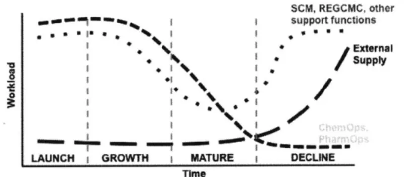
The proportional workloads of Technical Operations functions vary greatly over the lifecycle of a product (Figure 3). In the External Supply function in particular, Full Time Equivalent (FTE) resource usage ramps up exponentially as a product transitions from maturity to decline phase of the lifecycle. As products age and go off patent, the supply point decision is made to either continue producing the product at the existing site, transfer the entire manufacturing process to another site, outsource the product altogether, or eliminate/divest the product. The majority of these decisions will result in supply chain disruptions and introduce additional regulatory and operational risks. These risks will in turn translate into higher costs for Company X. The product themselves are not penalized for incurring additional costs since these operational costs are swept under the overhead rug with little visibility or clarity. Having a high mix portfolio where over 50% of the portfolio is comprised of these off patent products forces Company X to incur a much higher level of risk and cost than the product portfolio is actually worth.

SCM, REGCMC, other

.. I supportfunctions

*I External

I , 0Supply

LAUNCH GROWTH MATURE DECLINE

Time

Figure 3: Functional workload across Technical Operations over the lifecycle of a product

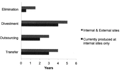
Lastly, the organization is not adequately structured to proactively handle lifecycle transitions and make supply point decisions prior to an actual supply chain disruption happening. The lack of standardized process and clear ownership for decision-making has resulted in Technical Operations carrying the burden of supporting a large number of non-strategic products awaiting elimination. The existing triage process for transfer, divestment, and elimination decisions is cumbersome, requiring many functional approvals and rework. A typical supply point decision can take upwards of eight months. Company X has attempted an organization-wide effort to drive down complexity in 20 10 and proposed over 900 tail end SKUs for product elimination.

These products largely still remains in the current portfolio as requests take so long to process and move through the workflow. Even after a decision is made, execution may take years to complete (Figure 4).

Elimination

Divestment

8 Internal & External sites

Outsourcing _{UCurrently produced at}

internal sites only Transfer

0 1 2 3 4 5 6

Years

Figure 4: Average timeframe to complete execution of supply point decisions

1.4 Project Objective

Given the pressures faced by Company X due to increasing operational complexity costs, the company has initiated this effort to gain cost transparency and use the generated data and model to more effectively manage the product portfolio composition.

The main objective is to identify the underlying factors driving complexity cost at the global level, quantify these factors into a cost model to be applied to specific business case evaluations and portfolio wide assessments. The key end user will be the Technical Operations organization carrying out both the decision-making and execution of supply point related matters. Critical design criteria will center on model accuracy, simplicity of user interface, and wide applicability for cross-functional stakeholders.

1.5 Hypothesis

Literature and previous projects indicate that operational complexity costs aside from direct production costs contribute greatly to the total carrying cost of a product, particularly towards the end of its lifecycle. We hypothesize that high complexity within an organization can be profitably reduced with the right information and implementation plan over time. Company X can reduce the total product complexity of its portfolio through increasing cost transparency, enabling it to be more strategic in regards to making supply point decisions and managing product lifecycle.

1.6 Thesis Structure

Literature Review

This chapter explores the work done on complexity management in the context of the

pharmaceuticals industry in academic papers and industry publications. The section also reviews past LGO projects related to complexity reduction at Company X and walks through the evolution of focus areas for tackling complexity and associated results. Lastly, we will summarize the approach and rationale for this project and how it builds upon previous work.

Approach

This section describes the methodology of building the complexity cost model in addressing product complexity. It details the analysis done to identify underlying factors of complexity cost generators and how these variables were quantified and incorporated into a general cost model. Also included is the approach to mapping out current state and proposing future state of supply point decision making process.

Results

This chapter summarizes the results from key pilot projects applying the complexity cost model and initial findings from a portfolio-wide screening. We propose some follow on topics and next steps for Company X.

This chapter discusses the shortcomings and limitations of the complexity cost model, along with additional considerations on the impact of implementation to Company X.

Conclusions

The final section covers the impact of the model on the future decision-making and operations of Company X and summarizes managerial implications for future complexity reduction efforts.

2 Literature Review of Complexity Cost Modeling

2.1 Defining Complexity in An Organization

Complexity has managerial implications for organizational performance, cost, and operational strategy. While practically important, complexity has not always been clearly defined. Concepts such as uncertainty and novelty have been associated with complexity, but does not aid in

understanding and addressing the issue. In the context of supply chain management, complexity has been parsed into detail and dynamic. Detail complexity is the distinct number of components or parts that make up a system (number of products in a portfolio, number of processes in a flow); dynamic complexity refers to a system's interconnected response to unpredictability [2]. Taking this one step further, the dimensions of complexity can be defined as multiplicity, diversity, and

interconnectedness of elements within a system. Multiplicity, a component of detail complexity, is the number of elements; diversity, also a component of detail complexity, is how differentiated elements are; interconnectedness, a component of dynamic complexity, is the interactions between elements and associated processes [3]. In application, complexity manifests different forms in products, processes, and people. In the context of products, multiplicity, diversity, and

interconnectedness can take on the form of product features, technology, and manufacturing platforms. In the context of processes, complexity is coordination across functions and different practices. In the context of organizations, complexity is the number of departments, differentiation of roles and tasks, or varying level of capabilities. These ideas become more concrete when we apply the dimensions to evaluate the supply chain operations for implications on risk, responsiveness, and cost [4]. Previous research has indicated that increasing product complexity increases inventory and decreases service levels [5]. In these particular studies, product complexity is defined as number of

SKUs. While previous literature established applicable definitions of complexity and complexity's importance in operations management, there has not been extensive work on application of complexity cost analysis and managerial implications in industry.

Complexity is desirable and necessary for many industries. New innovative products that meet evolving customer needs, smarter data management systems to reduce error are all added complexity that have benefited businesses and fueled industry growth. However, unnecessary complexity can inflate operational expenditures and compromise service levels. Complexity within a company is perceived to be highly qualitative and thus is difficult to isolate and define. Wilson and Perumal group complexity into three main categories: product, process, and organization [6]. Product

complexity refers to the existing collection of products and services offered by the company. Process complexity is all the steps, linkages, and handoffs required to deliver the products and services to the customer. Organizational complexity is the staff, structure, and governing policies put in place to execute delivery of products and services to the customer. Examples of each type of complexity are given in Figure 5.

Product Process Organization eIntroduction of *Coordination sCreation of new

product variations eDuplication and department

eLaunch of new rework *Matrix structure product eComplex SOPs for eMultiple reporting sOffering multiple decision making lines for single FTE

service packages to customers

Figure 5: The three dimensions of complexity and associated examples of each [6]

Often in an organization, all three dimensions of complexity co-exist and can be represented via a complexity cube (Figure 6). The interactions between the three dimensions drive observable effects

such as multiple unprofitable products, long lead times, product shortages, and low service levels. The impact of complexity is difficult to measure by virtue of the nature of complexity cost. These costs are not associated directly with a product. Beyond the financials, complexity can also generate

significant opportunity costs. Complexity costs increase geometrically and is not simply a function of the number of products in the system, but instead a function of the linkages between the products,

processes, and organization [7]. Since complexity cost is so difficult to measure and control, the ability to effectively manage it can become a company's greatest competitive advantage.

Organizational

Product

Process Figure 6: Illustration of the complexity cube

To understand the impact of complexity costs on the company, Wilson and Perumal propose to examine the profitability of a company. In a given product portfolio, only 20-30% of the products are profit generating while the remaining 70-80% of the products are actually

destroying profits (Figure 7). This whale curve represents the relationship between total products and cumulative revenue. As more complexity is introduced into the system, the rate of

complexity costs growth eventually erodes any additional value being created, resulting in an inflection point where profitability takes a downturn. Though this is never the case as reflected

by the typical financials. It can only be explained through complexity costs that do not factor into

the margin calculations for a product. In order to improve the overall profitability of the company, there are two options: reduce the cost of complexity or reduce the total amount of complexity in the system. Reducing the cost of complexity simply shifts the organization's position along the curve. Conventional methods such as tailed SKU reduction; lean and efficiency projects only move the needle slightly and alleviate some pressure by moving the organization upwards and leftwards on the whale curve. Reshaping or shifting the curve through eliminating complexity altogether from the system can achieve more significant results.

500%

Products that Products that

create proit"sep 300% .... %... % TOta 0% 0% 25% 50% 75% 100% % total products

Figure 7: General profitability curve of a product portfolio [6]

In summary, complexity arises naturally with the normal operations and growth of the business. Legacy products inherited from mergers and acquisitions, lost leader SKUs that enable the company to expand into new markets, and introductions of product variants to satisfy a broader range of customer demands are all examples of how complexity is continuously introduced into the system. Within the pharmaceutical industry, contractual obligations with health authorities and ethical concerns also contribute to companies taking on additional complexity that may not translate into positive profit or revenue. Over time, without active management and maintenance, the portfolio accumulates more profit-losing products and the total cost of complexity is more visibly felt throughout the company. The complexity exists along three dimensions: product, process, and organization. The cost of product complexity increases geometrically with the number of linkages within a network as more products and processes are introduced. The key challenge to managing complexity is indirect costs associated with complexity are not appropriately calculated or allocated. Most corporate accounting systems do not accurately capture complexity costs because of the existence of "catch-all" accounts that mask the true profitability. In order to reduce complexity, enterprises can either decrease the total amount of complexity, or make complexity cheaper.

2.2 Summary of Previous Complexity Reduction Projects

Previous efforts by Company X have focused on both reducing the total amount of complexity and on the cost of complexity. The first complexity reduction effort focused on product complexity. A

cross-portfolio analysis was done using financial and strategic criteria to isolate the low hanging fruits for elimination. These were the tail end SKUs [8]. Subsequent projects shifted from complexity reduction at a global portfolio level to local production site level. Efforts included identifying and dash boarding the various components of site-level inefficiencies, quantifying total manufacturing complexity costs trapped in the entire network of production sites by comparing a single SKU plant versus a multiproduct plant [9], [10]. These projects have kept the spotlight on complexity reduction within Technical Operations and allowed the organization to tackle all three dimensions of complexity at both a corporate scale and individual production site level.

This project continues to build upon the previous work. The focus shifted from being more

theoretical to being more applicable. The complexity model developed is able to perform brand and SKU-level evaluations of supply point decisions, incorporating sensitivity analysis to enable the user to use the tool for specific business cases and general portfolio assessments. Work to date has taken a top down approach to quantify complexity costs, versus this project, which takes a bottom up approach in data collection and model construction.

2.3 Review of Methodologies Used in Complexity Cost Modeling

To quantify the complexity costs for a product, several approaches were evaluated. The pros and cons offered by each approach, and the executional feasibility given time constraints were used to choose the optimal methodology for this project.

Mixed Integer Linear and Nonlinear Programming

Application of linear programming to model the entire pharmaceuticals supply chain is frequently cited in academic literature. Mixed integer linear programming (MILP) and mixed integer nonlinear programming (MINLP) formulations have been used to represent the key components of the supply chain with the objective function to maximize net present value or gross margin and constraints on production capacity, allocation, inventory, mass flow, and non-negativity [11]. Complexity in a system is typically quantified by the change in cost or profit. This methodology is used to model complexity by measuring effects of individual variables on minimizing cost or maximizing profit. Other variations of the model include introduction of new products to evaluate impact on supply point decisions, incorporation of demand data to optimize capacity planning, and accounting for

opportunity cost of working capital associated with inventory [12]. Monte Carlo simulations are typically used to capture the complexities and risks in key variables. While the MILP/MINLP approach effectively models the entire supply chain system, it is extremely complex to develop. The interdependency of the model components requires many data inputs and deep knowledge of market, product, and manufacturing information (Figure 8). More importantly, the model's core is based on a systemic approach and does not plainly isolate the complexity costs at any single point within the supply chain.

USER INTERFACE

DATABASE

INPUTS OUTPUTS

" Cost data * Expected portfolio cost

" Durations * Expected portfolio NPV

Resource requirements Nurtfoloprodr *Product demands Nme fapoe rg

*Manufacturing data *Frequency distributions for portfolio

*Phase transition probabilitiesmers

Technical failure probabilities a Efficient frontier * Market and financial data & Resource utilisation

* Uncertainty data

DRUG TASKS RESOURCES

PORTFOLIO

" Drug 1 0 capital

" rg2LvlIBiopharmacuia * In-house

Drug 23ee Dev nt Portfo ca

* Personnel

e Contract Level 2 D D 2 Dru 3 manufacturing

Level 3 | Phase I H Phase 11l Phase liIIl Market search

organisatIon

Level 4 JDevelopmentj [Manufacture Cinical Trialsi

Figure 8: Sample schematic of a typical MILP supply chain model [13]

Activity Based Costing

To extensively target only a subset of costs, another methodology to employ is activity based costing (ABC). ABC is driven by the need to accurately reflect the relevant cost information needed for decision-making. This approach traces both direct and indirect expenses to the corresponding products, services, and customers that incur the costs [14]. In matrix

organizations, multiple functional involvements across often-different geographical locations are required to deliver the final product or service to the customer. Traditional accounting techniques capture fixed and variable costs to manufacture the product or service and then allocates

overhead based on some generalize rule. This has been sufficient for the 1950s' traditional companies. As companies shift to becoming more integrated in the 1990's, offering a greater

variety of products and services through more diverse distribution channels, the indirect costs become much more prominent and require proper traceability and assignment (Figure 9).

Changes In cost structure 100%... 90% E 80% 70% w Indirect Expense 60% (overhead) E 50% E 40% / Direct Material 30% 20% Direct Labor 10% 0%

Figure 9: Indirect costs are displacing direct costs in integrated businesses [14]

In order for ABC to be useful, it must comply with the realities of the organization. The relevant resource and activity drivers chosen should correctly represent the cost structures and activities in the supply chain. This could be challenging at times because parts of the data required are quantitative translations of qualitative activities. A key point to note with ABC is although the model may not be as sophisticated as the MILP/MINLP approach it does provide the sufficient relevant information for decision-making purposes [15].

Data Mining and Decision Tree Software

The final approach evaluated to identify and capture complexity costs is to relook at existing data through new lenses. Because complexity costs are often hidden and unsorted, a simple solution may just be to extract out only the relevant pieces of information. By defining new metrics, the impact of complexity becomes more visible. Automated pattern detection software can serve the purpose of revealing connections in data and exposing patterns not readily detectable by

traditional accounting methods [16].

Analytics can process and make sense of large volumes of raw data and make actionable

and managing complexity easy, the software infrastructure and support needed would be highly capital intensive and may be a deterrent for adaptation. Decision trees provide a framework to enable management to evaluate options quantitatively, taking into account systematic risks and uncertainties. By enabling better decision-making, decision tree tools can decrease the costs particularly associated with process and organizational complexity [17]. Decision trees have been widely used to model the decision-making process in both product design and supply chain management applications. Probabilities of events that can impact a supply decision and the financial cost associated with the uncertainties can be captured by the decision tree through expected cost functions and the optimal decision determined from the function [18]. Decision trees can also be used for multi-stage analysis with uncertainties to minimize total expect cost

[19]. Given the versatility and comprehensiveness of decision trees, it can be a powerful tool in

cost analysis.

Selection of the desired approach balanced level of model sophistication and accuracy and the feasibility of execution given the limited project duration and access to needed data and information. Also, usability is another crucial concern. Models that required special software licenses and extensive programming or functional knowledge pose high barrier for adaptation and would not be the ideal choice in this case. Given budget, time, and implementation constraints, Excel and decision tree commercial software was chosen as the backbone to

construct the model. Excel requires no specialty training and the ease of use allows flexibility in model construction and modification. A single commercial software license was obtained to pilot the feasibility of using the developed model to enable decision making across multiple functions within Technical Operations.

3 Approach to Quantify and Model Complexity Costs

3.1 Approach Summary

Company X faces particular challenges in product and process complexity. Chapter 3.2 focuses on the approach to address product complexity. The design of the approach is systematic,

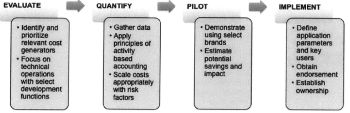
recommendations are derived from testing of the theory using case studies. This approach translates into the major phases for the thesis work (Figure 10). The primary phase focuses on identifying the cost drivers within Technical Operations. How to define and prioritize the complexity cost generators are detailed in Chapter 3.2.2. Once the cost drivers are prioritized, they are generalized into a usable model, which is then piloted with select case studies. This is covered in Chapters 3.2.3 - _{3.2.10. Chapter 3.3 focuses on the approach to address process}

complexity. Through current state mapping of lifecycle management decision-making process, we clarify the weak points and make recommendations for reformation. Organizational

complexity is briefly discussed only in consideration to its effects on product and process complexity in Chapter 3.4 It will not be investigated in detail within this thesis work.

EVALUATE QUANTIFY PILOT _IMPLEMENT

* Idenity and -Ghr data -Deona-afle 00e*f

pliorgize . Apply usfng siewd appka

rssvawt cost ponwIpes or branEs pa"ramoS*

geneators actM*y Esthale andkey

* Focus on based poteiAs UsIr

tal acc-nng sawn an -Ot4m

operan -sale costs kmpac andorseent

Wth SOWec approriat"y Est~bs

deve4Opment _{Wtah iSk}

ownroIp

Uznctiona _atr

Figure 10: Summary of thesis approach and project phases

3.2 Product Complexity

To validate the hypothesis that operational complexity costs contribute significantly to the total carrying cost of a product, we need to formulate an accurate account of cost drivers. This is achieved through a complexity cost model via activity-based accounting.

Complexity cost rises proportionally to transactions. High variability in products and services increases the total transactions and activities within the organization. The focus of product complexity cost is on these transactional activities within Technical Operations. Company X uses consolidated Total Product Cost (cTPC) to measure the raw material, labor, and production overhead of a product. The transactional costs are not directly incurred through manufacturing and thus fall outside of cTPC. Instead, they are captured within functional budgets, global

overheads, and non-production accounts. To extract these costs, we have to define the activities that generate them. These activities become 'complexity cost generators'.

3.2.1 Classification of Complexity Cost Generators

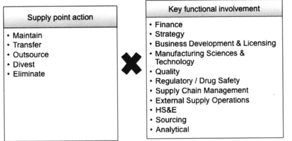
We start with supply point changes that initiate a cascade of activities within Technical Operations global functions. The most common supply point actions during the mature and decline phases of the product lifecycle are summarized in Figure 11. Each action requires support from corresponding functions involved. Within each function, a series of activities are performed for each corresponding

supply point action. We then further break down these activities into tasks that can be quantified by

FTE hours. The smallest unit of complexity generators is the task, which are performed to

accomplish activities required for each supply point action within various functions.

Key functional involvement Supply point action

-Finance -Maintain * Strategy

* Transfer .Business Development & Licensing -Outsource * Manufacturing Sciences &

- Divest Technology

- Eliminate -Quality

-Regulatory / Drug Safety - Supply Chain Management - External Supply Operations

- HS&E -Sourcing * Analytical

Figure 11: Identifying cost generating activities by functional involvement in supply point actions

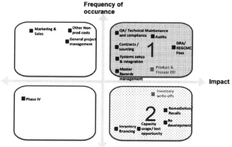
Once the cost generators are identified, the tasks are filtered and ranked based on the frequency of occurrence and the financial impact. Those tasks that are required on an annual basis, such as

product stability testing, complaints handling, quality and HS&E audits, etc. are classified as high frequency. High impact is measured by the FTE hours consumed and the amount of fees and expenses required to conduct the activity. Low frequency, high impact tasks occur infrequently, but when they do, can contribute significantly to complexity costs. An example of high impact and low frequency cost generator is redevelopment cost of existing products that involve bioequivalent studies, which are rare but can amount to upwards of millions of dollars. Others include capital cost of inventory financing and holding; remediation costs for plants, equipment, or site; and opportunity

cost of capacity allocation to a low profit product. The model will focus on high impact and high frequency items. We choose to provide guidelines to identify if these factors are in play for specific cases and how to gather the data needed to assess them (Figure 12).

Frequency of

occurance Markeft& OM NO

Saes -~ CO0tS

I Impact

Figure 12: Classification of complexity cost generating tasks by impact and frequency of occurrence

The preliminary assessment of cost generators also included indirect costs such as the financing cost of excess safety and bridging stocks due to forecast errors, Phase IV clinical trials, and marketing. For single sourced, chemical, solid oral dosage form products, Company X maintains a target total safety stock of 30 weeks. This is broken down into 18 weeks of Drugs Substance, 8 weeks of Drug Product, and 4 weeks of Finished Product. For a typical slow moving, end of lifecycle product, there is almost zero marketing and Phase IV costs. The capital cost of 30 weeks of safety stock is valued at the consolidated total production cost of the DS, DP, and FP, which is dependent on the product. Finally, warehousing costs are negligible since majority of these end of lifecycle products are produced at fully depreciated and Company X-owned sites. Through initial evaluation, these costs were demonstrated to be minimal compared to the high impact and high frequency cost generators and were thus not included in the evaluation and cost model.

3.2.2 Data Gathering

There are two main contributors to the cost of an activity: 1) the FTE resource required to execute the activity and 2) the expenses and fees not directly tied to human resources required to support the

execution of the activity. Both pieces of data can be obtained through either accounting invoices or interviews with employees and managers who do the work.

The most direct way to gather the FTE resource usage data is to first break down the supply point action into activities and then decompose the activities into smallest units of discrete tasks by function. Taking an example of the supply point action of 'maintain' Table 1 details the activities required to carry out maintaining a product on an annual basis and all the tasks associated with each activity. The involved functions then provide an estimate of the FTE hours and expenses per task per time that it is performed. If a task is performed on a frequency of greater than one, then the FTE hours will warrant a multiplier. Translating the total FTE hours into dollars and aggregating the fees, we can obtain the total cost of activities and ultimately supply point actions that are driven by product complexity. The advantage of knowing the cost of the smallest unit of activity is the ability to reconfigure and customize costs accurately for unique scenarios.

Table 1: Example of data collection process for complexity cost generators

DISCRETE FTE HOURS FUNCTION

ACTIVITIES EXPENSES/FEES

TASKS PER TASK

Manufacturing Annual validation

IFTE x 3 days Science &

including reportsTechnology

Manufacturing

Technical Troubleshooting 5 FTEs x 2 days Science &

onsite

Maintenance Technology

Annual stability 0 Cost of stability Analytical

testing test

Supplier relations External Supply

team support Operations

cGMP / quality Travel expenses Quality Assurance

2 FTEs x 5 days

audit and fines

HS&E technical Travel expenses HS&E

Annual audits ₁ FTE x 5 days and fines

audit and visitadfie

Follow up and 3 FTEs x 2 Quality

Table 1: Example of data collection process for complexity cost generators

Review contracts Sourcing

Contract and make any IFTE x 3 days

Maintenance needed changes

Follow up with iFTE x 3 Sourcing

issues, negotiations days/month

In instances that data is not reliable for singular tasks and the FTE resource allocation is very distributed within a department, an estimation approach is taken to arrive at the cost per brand per year of a task or activity.

3.2.3 Basic Structure of The Complexity Cost Model

Following the identification, classification, and quantification of the key cost generators, it is

important to turn this information into a useful format for to enable decision makers to apply the data as suitable for their needs.

It was previously stated that reducing product complexity requires both portfolio-level optimization and individual business case evaluations to cut the non-profitable and nonstrategic product offerings. The intent of the model output is to provide users with a systemic level view and also a specific tool

to assess distinct decisions.

The complexity cost model ultimately feeds into a decision tree and also into a Net Present Value (NPV) analysis (Figure 13). The decision tree encompasses the indirect costs of all possible supply point decisions that can be made for a particular product so the user can compare the financial implications of each with regards to complexity. The choices that the tree makes are supply point decisions that would result in possibly incurrence of complexity costs for the product. Because the tree incorporates risk factors and data specific to a product, the decision tree is a tool used at the individual brand level. The expected value of each possible path down the tree is calculated and the model can identify the minimal cost supply point decision for a product at a systemic level. The NPV analysis is intended to evaluate a single supply point decision, incorporating complexity cost

data with existing financial data from Company X's S&OP system to provide a comprehensive view of the long-term impact of a decision.

Direct Costs indireactts Consolidated Total Fees, expenses. personnel Prdcto Cost

Maintenance Outsoutrcing X/cio / _________

Work Activities

Figure 13: Complexity cost model structure

The decision tree component of the model uses a commercial program called TreeAge Pro, which is software with the capability to model entire systems and choose the optimal path depending on calculated end node value. Details behind the construction of this decision tree logic are described in Chapter 3.2.7. This program enables the user to simultaneously evaluate the payouts and costs of all outcomes. The model also takes into account probabilities of success and failure for specific events, such as outsourcing, and calculates the final expected value. The commercial software also has the ability to perform sensitivity analysis around chosen nodes, exclude certain paths in the analysis, and use distributions instead of absolute probabilities for the occurrence of events.

The NPV component of the model is built in Microsoft Excel and is adapted from the finance

Capital Appropriation Request (CAR) form, using current budget rates. It takes into account the cash inflows and outflows from impact on net sales, avoided costs, and incremental costs.

In combination, the two components of the model are able to provide a comprehensive overview of the financial aspects of a change request with comparative and sensitivity analysis to ensure a complete business case can be generated.

. .... ...

7-t

z T T T W

3.2.4 Other Considerations for The Model

A critical design criterion for the model is user interface. There were two purposes the user interface needs to achieve: ease of navigation with limited training on the model, and minimal number of inputs required to run the model. Commercial software is selected for the decision tree and Excel is selected for the NPV analysis based on the familiarity and intuitiveness of the programs. The model will incorporate a large amount of inputs, yet be simple to use for ease of knowledge transfer and sustained application.

The majority of the model has basic assumptions prebuilt into the cells and changes are auto populated based on user input. User will only be required to assemble and prepare the quantitative and qualitative information outlined in Appendix 1.

Depending on the needs of the user, model input can be as simple or as detailed as desired. Appendix 2 shows the generic input interface. All cells in red are the required user inputs. The user only has to indicate anticipated occurrence of relevant lifecycle activities for the next five years and the model automatically calculates the annual complexity costs based on assumptions for a medium risk product. Once the annual total complexity costs are calculated, that data will automatically feed into the NPV model. Should the user want another level of granularity, there is the option to select only the relevant tasks for each lifecycle activity. This is a secondary layer in the Excel model, where all tasks are visible and can be included in or excluded from the complexity cost calculation. The risk level for the product under evaluation can also be modified as desired.

3.2.5 Incorporating Risk and Uncertainties into The Model

There are several sets of scaling factors used to adjust the complexity costs and the uncertainties in the model. The first set of factors adjusts for risk. The level risk is evaluated across technical, business, regulatory, and operational categories, applying failure mode and effects analysis (FMEA) and supplier assessment methodology. There are three levels of risk classification: low, medium, and high risk categories; each corresponds to a multiplier on complexity costs. The risk scaling factor is incorporated to appropriately adjust the complexity costs obtained via ABC since the cost figures are average numbers and has a large range across low to high scenarios. The risk factors considered are summarized in Table 2. The risk factors are first rated on severity (scale of 1-7), occurrence (scale of

1-5), and detection (scale of 1-7). The product of these three ratings becomes the standard risk

priority. Each risk factor is then scored on a 0-100 scale. An example of the risk factor scoring system for manufacturing technology is provided in Table 3. Finally, the risk factor utility is calculated by multiplying the risk factor score by the risk priority. The risk priority weighting is initially equal for all categories, but can be prioritized by the user, which will then change the risk factor utility. A product with risk factor utility value between 0-25 is deemed low risk, 26-50 is medium risk, and 5 1-100 is high risk. The multipliers assigned to the risk levels are 1.0, 1.05, and

1.5 respectively. This is based on both observations that complexity costs increases geometrically

and also the range of data received through activity-based accounting.

Table 2: Risk factors by category to scale complexity costs

RISK CATEGORY RISK FACTORS

Technical Manufacturing Technology

Process capability/ validation Analytical methods

Strategic Strategic positioning

Demand volatility / existing competition Life saving medicine?

Regulatory Number of markets and regions of sale Documentation completeness and compliance Registration compliance

Operations Footprint & capacity

Supply Chain

Contractual Obligations

Table 3: Example of risk factor scoring scale

Risk Factor Scoring Scale

Low High

0 25 50 75 100

Film Coated Transdermal Biologics, cell

Hard Gelatin Tablets, Sugar Therapeutic therapy, Advanced

Tablet

Capsules Coated Tablets, Systems, sterile Therapy Medicinal

The other set of factors is incorporated to reflect the uncertainties in the execution of supply point actions. Success means that the process reliability, quality, and integrity of the product produced at the new site is the same as the old. On supply point actions such as manufacturing transfer and divestments, successful outcome is not guaranteed. Thus a probability is assigned to calculate expected costs for internal to internal, internal to external, external to external, and external to internal site transfers. These probabilities were converted from Company X's Product Improvement Portfolio (PIP), which tracks risks within manufacturing, analytical, regulatory, and product quality. The probabilities are then adjusted accordingly for low, medium, and high risk products.

These scaling factors are quantitative within the model, but qualitative in nature and origin. It remains up to the discretion of the user to update and adjust as needed.

3.2.6 Building The Net Present Value Model

The aggregated complexity cost data from ABC feeds directly into a five-year NPV model. The base scenario evaluated by the NPV model is for product elimination, assuming 100% total loss in sales for the next five years. The model is set up with reversed cash flows. Cash 'inflows' that contribute to a positive NPV are the potential savings in complexity costs and all other costs incurred if the product was not eliminated; cash 'outflows' that contribute to negative NPV is the projected net sales not generated due to the elimination of the product. If strategies are in place to partially recover some of the sales or deplete existing inventory, the user can make modifications to the NPV model.

3.2.7 Building the Decision Tree Model

A decision tree maps all out potential outcomes of every single decision within a system. The basic structure of decision trees consists of branches and nodes. Each branch represents a different outcome or decision. Each node defines the properties of the attached branches. Commonly used node types are decision nodes, chance nodes, and terminal nodes (Figure 14). The decision tree can account for uncertainties via the chance node, where the user defines probability of success associated with the outcome. Terminal nodes indicate end of decision and

there must be a final payout value associated with each terminal node. The payout value can be defined as a function of variables or as an absolute value.

Chance 4 Terminal

o

Figure 14: Decision Tree basic structure

The use of the decision tree model gives user a systematic view of all possible strategies and compares the cost and benefit tradeoff to enable optimized problem solving. The logic in setting up the model is to enable every strategy that is relevant for a product to be visible, allowing comparison in cost with respect to key variables and uncertainties within the organization. The model is set up with differentiators to isolate the particular problem at hand. Because small molecules and biologics vary so greatly in cost, technical and supply attributes, that is the first differentiator. The focus of this model and project is on small molecules. Within small molecules, the cost of each strategy is driven mainly by the riskiness of the product and the stage in the supply process (DS, DP, FP, and brand). The product risk profile is defined next, from low, medium, to high risk. Risk classification is address in Chapter 3.2.5. The user has the option to run only one risk level or multiple to compare the sensitivity of the cost to risk classification. The next level of differentiator is the stage in supply process. The cost of lifecycle activity management is incurred at 100% at the brand level, but only partially at the DS, DP, or SKU level. The unit defines how much of the total brand cost should be taken into account. Finally, for each unit in the product supply process, the possible strategies are: continue existing or maintain, transfer, outsource, prune, or divest. Maintain means continuing with the current manufacturing and supply of the product, incurring full carrying cost and any additional cost associated with the strategy. Within transfer, there are four permutations of internal and external transfers with associated uncertainties of event success. Outsourcing is defined as the cost of buying product and services directly from a third party.

Figure 15. The variables and costs are defined upfront, which gives user full flexibility to modify once and automatically carry throughout the calculations in the entire decision tree. The

uncertainties, or random variables in each strategy as defined by the probability of activity success (for example the success rate of an internal transfer) are also defined upfront and only need a one-time alteration to propagate throughout the entire decision tree. The risk classification of the product splits the decision tree into three main branches, allowing the user to progress down a single chosen branch or run all three simultaneously as a comparison. Finally, there is the option to run the model at the brand, DS, DP, and FP levels by excluding the irrelevant branches from the strategy.

Ultimately, the model generates the expected costs of all decisions within the system accounting for all uncertainties, using the pre-defined variables.

The decision tree model calculates all expected values of every feasible supply point

decision, accounting for uncertainties. To consolidate all the various scenarios into a single model, the various risk levels are built as branches off a single tree. In application, the user would choose which risk level to run the analysis on. Within each risk level, the tree then branches to all the product stages that decisions can be made on (

Figure 15). For a typical pharmaceutical product, a supply point decision can be made at the Drug Substance (DS), Drug Product (DP), Finished Product (FP), or brand level. DS is the active ingredient in the product, DP is the stabilized complete formation of a product, and FP includes all primary and secondary packaging and labels. Company's X accounting system only provides costs for SKUs, which accumulates costs through raw material, DS, DP, and FP stages. In order to reallocate this total cost back to individual stages of a production cycle, a set of adjustment factors were created. Since the complexity costs are mainly calculated at a brand level, a certain percentage is taken for DS, DP, and FP. The percentages are allocated to reflect exponential complexity cost increase with progression up the manufacturing and supply chain. At the DS, DP, FP, and brand level, there are the same sets of decision that can be made: continue production at existing site, transfer, outsource, eliminate, or divest (only for brand). Then the expected complexity costs for each outcome is calculated. Computing the model results in choosing the lowest cost path. The user

can freely adjust the cost generators relevant for the product under evaluation. The probabilities of transfer success and risk scaling factors are set on the default level but can be modified.

4.II0 VI cL E 0 0,0 0 0L U0 M C 00 0 20 0

Figure 15: Skeleton of decision tree model 3.2.8 Data Validation

The model construction was performed via a bottom up approach, aggregating data pieces through activity-based accounting. The final cost for all lifecycle activities per brand per year is estimated from costs of single functional tasks, the smallest unit of activity. Data validation takes a top down approach. The total spends for an entire department, including global and local budgets are captured. Within the total budget, there are overhead support and other SG&A expenses. For model validation, we only want the amount allocated solely to product management. This can be taken as a percentage of the total budget. That percentage will vary based on function. The exact percentage is verified through existing key projects and information gathering from functional heads and key people that perform the work. The total spend budget for brand lifecycle activity management is then divided by the total number of brands to arrive at spend/brand for that particular function. This number should be on the same magnitude as the bottom up number (Figure 16).

pe Total budget/spend for the

brand entire department

$ aggregated percentage of total

spend dedicated to

for iffecycie 4lifecycie,

management at management

brand level activities

$ for individual activities by $ per

function _ran

Figure 16: Model validation schematic

A major consideration in building the model from the ground up is inclusiveness of all relevant

data, which is why it is important that the final number derived from the bottom up approach is sense checked. As detailed in Table 4, the aggregated cost per brand closely matches a heuristic calculation done via a top down approach. It is not critical that the numbers match exactly since there are a series of assumptions used in performing the calculations. The magnitude is what we