Mixing intensification under turbulent conditions in a high pressure microreactor

HAL Id: hal-02318108

https://hal.archives-ouvertes.fr/hal-02318108

Submitted on 6 Jan 2020

HAL is a multi-disciplinary open access

archive for the deposit and dissemination of

sci-entific research documents, whether they are

pub-lished or not. The documents may come from

teaching and research institutions in France or

abroad, or from public or private research centers.

L’archive ouverte pluridisciplinaire HAL, est

destinée au dépôt et à la diffusion de documents

scientifiques de niveau recherche, publiés ou non,

émanant des établissements d’enseignement et de

recherche français ou étrangers, des laboratoires

publics ou privés.

Mixing intensification under turbulent conditions in a

high pressure microreactor

Fan Zhang, Samuel Marre, Arnaud Erriguible

To cite this version:

Fan Zhang, Samuel Marre, Arnaud Erriguible. Mixing intensification under turbulent conditions in

a high pressure microreactor. Chemical Engineering Journal, Elsevier, 2019, 382, 122859 (12 p.).

�10.1016/j.cej.2019.122859�. �hal-02318108�

Mixing intensification under turbulent conditions in a high pressure microreactor

Fan Zhang

, Samuel Marre

, Arnaud Erriguible

1_{CNRS, Univ. Bordeaux, Bordeaux INP, ICMCB, UMR 5026, F-33600, Pessac, France.} 2_{CNRS, Univ. Bordeaux, Bordeaux INP, I2M, UMR 5295, F-33600, Pessac, France.}

Abstract

The turbulent mixing of two miscible fluids is investigated in a high pressure (HP) coflow mi-croreactor operated at 100 bar. Ethanol and CO2 are selected as model solvents to mimic the

final targeted application, i.e.: a supercritical antisolvent process at microscale (µSAS). We first demonstrate experimentally that turbulent mixing can be reached in a microchannel using HP microfluidics. A computational fluid dynamic (CFD) model, performed using direct numerical simulation (DNS) down to the Kolmogorov scale has been applied for the turbulent mixing simula-tions. The effects of the main operating parameters on the final mixing efficiency has been studied, namely: the temperature, the fluid flowrates, the microchannel dimensions and the capillary inner and outer diameters. According to a predefined intensity of segregation, the characteristic mixing times are determined and used for determining mixing efficiency. The ratio of the total mixing time to the diffusion time depends on the ratio of the kinetic energies (the outer fluid to the inner one). The obtained micromixing times have been related to the turbulent energy dissipation rate ϵ, calculated directly from the velocity fluctuations. The mixing intensification is obtained with much lower characteristic mixing times in the microreactor (one order of magnitude) than previously reported. This fundamental study is an indispensable guidance for several processes, including the

µSAS applications.

Nomenclature

A area m2

D diffusion coefficient m2_{· s}−1

DID inner diameter of capillary µm

DOD outer diameter of capillary µm

Dh hydraulic diameter µm

E engulfment rate s−1

Im intensity of segregation

Lp larger side length of trapezoidal channel cross-section µm

Ls smaller side length of trapezoidal channel cross-section µm

N Total number

P e Péclet number for mass transfer

Q flowrate m3_{· s}−1

R ideal gas constant J· kg−1· K−1

RID inner radius of capillary µm

ROD outer radius of capillary µm

Re Reynolds number

Sc Schmidt number

T temperature K

V molar volume m3· mol−1

g gravitational acceleration m· s−2

u velocity vector m· s−1

a first coefficient in Peng–Robinson equation of state

b second coefficient in Peng–Robinson equation of state

d depth of microchannel µm

kij, lij interaction parameters in Peng–Robinson equation of state

l mixing channel length m

p pressure bar

t time s

td time delay of the first order system s

tm mixing time s

tv hydrodynamic lifetime of vortex s

u absolute velocity in x direction m· s−1

v absolute velocity in y direction m· s−1

w absolute velocity in z direction m· s−1

x mass fraction

Greek symbols

α α function in Peng–Robinson equation of state

ϵ energy dissipation rate W· kg−1 or m2_{· s}−3

λ microscale µm µ dynamic viscosity P a· s ν kinematic viscosity m2· s−1 ω acentric factor ρ density kg· m−3 Subscripts

0 initial conditions (initial temperature of pumps for fluid flowrates and temperature in channel for fluid velocities) B Batchelor c critical point E engulfment EtOH ethanol in inner fluid K Kolmogorov

m mixture

1

Introduction

Fluid mixing is a common and essential process in chemical engineering, especially for fast reactions as competitive reactions and particles precipitation. For example, in antisolvent precipitation processes, a fast mixing is needed in order to precipitate small and homogeneous particles, while avoiding large gradients of supersaturation in the reactor. For this reason, it is critical to investigate the mixing of solvent and antisolvent to meet this requirement. In a previous study, the laminar mixing of supercritical CO2 and ethanol in a high

pressure (HP) microreactor has been discussed [1]. The obtained results emphasize the capability of such coflow micromixer to reach short mixing times in the order of the millisecond, even in laminar conditions. One of the main limitations of classical micromixers is the difficulty to reach high flowrates to access turbulent conditions, which greatly favor mixing. Indeed, high flowrates generate high pressure drop in the channel and generally result in the breakup of the microchip. Nevertheless in another study [2], we have shown that our HP microreactors were able to reach purely inertial (turbulent) conditions in immiscible two phase flow conditions. According to the concentration spectrum for liquid mixtures as a function of length scales, the turbulent mixing can be divided into three distinct stages, inertial-convective, viscous-convective and viscous-diffusive subrange [3]. The inertial-convective stage corresponds to fluid mixing among and inside eddies from the largest scale down to the Kolmogorov scale λK. Fluid kinetic energy is passed through the deformation and reduction

of eddies without molecular diffusion, so concentration variance still remains significant and the mixing is incomplete in this stage. While the considered length is reduced in the range between the Kolmogorove scale

λKand the Batchelor scale λB, the viscous-convective mixing occurs mainly by laminar strain. In this subrange,

the eddies disappear and the concentration variance drops dramatically, leading to high efficient mixing. The viscous-diffusive mixing is active for the subrange smaller than λB and species mixing is achieved mostly by

diffusion. The micromixing is predominantly related to the molecular mixing in the viscous-convective range below the Kolmogorov scale. As precipitations and chemical reactions take place at the molecular length level, a special attention should be paid to the micromixing.

However, it is quite difficult both experimentally and numerically to observe directly the micromixing in a turbulent flow down to microscales. Therefore, experiments implying the use of competitive reactions have been designed for detecting the micromixing by an indirect way among which is the iodide iodate reaction, also known as Villermaux-Dushman protocol [4]. Based on experimental results, several micromixing models have been proposed: the generalized mixing model (GMM) [5], the interaction exchange with the mean (IEM) [6-8] or the engulfment, deformation and diffusion model (EDD) [9]. These models have been compared and applied to qualify the micromixing [10] but experiments are always needed to validate modeling results. The EDD model has been proven to be capable of providing more precise results compared to other models [11]. So, the micromixing time, as a criterion to characterize mixing quality accepted by most researchers in this domain, is the engulfment time of the EDD model. It is based on the fluid deformation and diffusion in micromixing scales [12], and defined as:

tm= 1 E = 17.24( ν ϵ) 1 2 (1)

with E the engulfment rate, ν the kinematic viscosity of fluid and ϵ the energy dissipation rate of the turbulent flow. The coefficient 17.24 results from the engulfment rate and this coefficient has been deduced by Baldyga and Bourne from the hydrodynamic lifetime of the corresponding vortex (a value of this coefficient of 12 is theoretically admitted) [3].

The objective of the present work is to study the turbulent micromixing of CO2and ethanol in a homemade

silicon-Pyrex microreactor with a coflow geometry selected to provide correct guidance for the µSAS process [13], which consists in a fast precipitation process resulting from fluids mixing. The originality of this study is that the turbulent coflow mixing has been performed and first observed experimentally in the microreactor at 100 bar and further characterized and investigated with a numerical simulation in order to quantify the mixing. Thanks to the small dimensions of the microchannel, the direct numerical simulation (DNS) or quasi DNS has been used to describe the hydrodynamics of turbulent mixing under isothermal conditions. This approach allows for catching all (or almost all) mixing scales involved in the process, and specially the micromixing scale. This is made possible by the use of a High Performance Computing code developed in our laboratory. The CFD model has been validated in a previous work. Based on the simulation results, several operating parameters have been examined, namely: the temperature, the initial velocity ratio, the Reynolds number and the microchannel dimensions. The characteristic mixing time is estimated and compared to the micromixing time (Equation 1).

2

Experimental section

The turbulent mixing of ethanol and CO2 has been observed in a coflow high pressure microreactor at 20 ◦_{C and 100 bar to demonstrate experimentally that turbulent regimes can be reached in those conditions in a}

confined environment.

2.1

Experimental set-up and procedures

The microreactor has been designed for µSAS precipitation so that a full 3D coflow geometry was selected to prevent plugging due to particles formation and potential interactions with the walls. The configuration was printed on a mask for the UV exposure of a spin coated photoresist layer on the surface of a silicon wafer. Then, the 2D microchannel design was extruded in the third dimension by a wet etching procedure on silicon. Eventually, a top transparent Pyrex cover, offering optical access for the camera, was anodically bonded to seal the device. The final microreactor is illustrated in Figure 1. The microreactor is then inserted into a general set-up described on Figure 2. The CO2used in the experiment is purchased from Messer company and the 96%

ethanol is supplied by Xilab. The CO2 injection is performed with an ISCO 100 DM pump equipped with a

cooling jacket in which the temperature is constantly maintained at -5◦C by a cooling fluid and the ethanol is injected by a Harvard PhD 2000 high pressure syringe pump. Another ISCO pump of the same model is used as a back pressure regulator to control the downstream pressure fixed at 100 bar. A high speed camera, Phantom Miro Lab340 of Vision Research company, is implemented in the set-up, which has a maximum resolution

of 2560 × 1600 with a pixel pitch down to 10 µm and a minimum exposure time of 1 µs. This camera is connected to a ZEISS Axiovert 200M microscope with a 20× magnification objective. The CO2is injected into

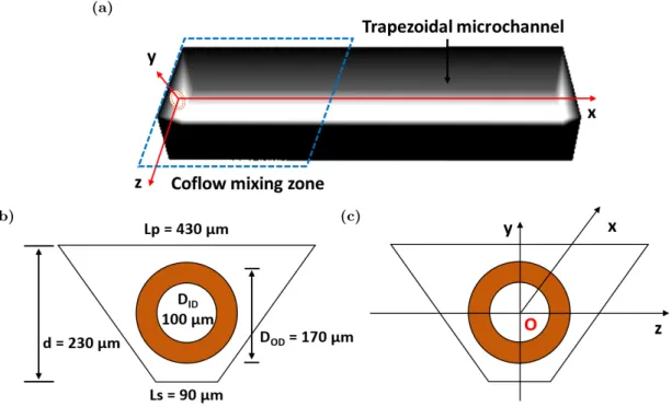
the microreactor inside a preheating channel to ensure that it reaches the desired temperature conditions. Then, it is allowed to encounter the ethanol flow, which is injected through a capillary inserted inside the observation microchannel, resulting in a full 3D injection mixer (see Figure 1, cross-section view). The silica capillary outer diameter was selected to fit with the internal dimension of the channel. After its insertion, it is epoxy-glued to the microreactor to ensure a perfect sealing and a use at high pressure up to 150 bar.

Figure 1: Illustration of the high pressure microchip made of silicon-Pyrex and the trapezoidal channel with an inserted capillary.

Figure 2: Experimental set-up for the observation of the turbulent mixing in the microreactor under high pressure.

2.2

Turbulent mixing observation in the microchannel

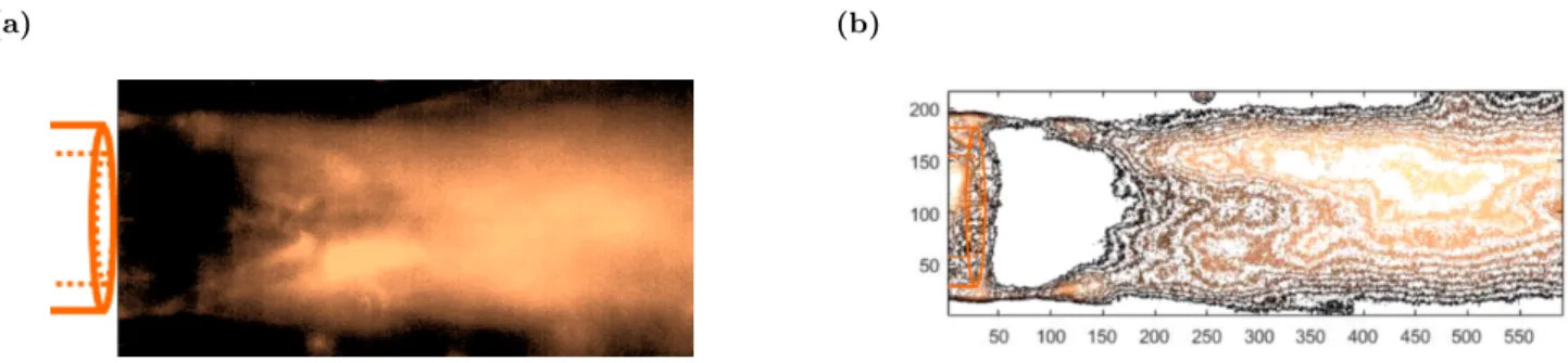
An instantaneous view of the turbulent mixing occuring at the capillary tip is shown on Figure 3. The dense CO2, the outer fluid, encounters the inner fluid ethanol at 20◦C and 100 bar. The fluid flowrates are

7000 and 800 µL/min for the CO2 and the ethanol, respectively, resulting in an analytical average velocities of

camera with a recording rate of 10000 images per second (see video 1 in supplementary data).

Figure 3: Instantaneous view of the CO2-ethanol turbulent mixing, captured by the high speed camera, for conditions

QCO2 = 7000 µL/min, QEtOH = 800 µL/min, T = 20

◦_{C, P = 100 bar.}

(a) (b)

Figure 4: Processed images of CO2-ethanol turbulent mixing in the microchannel: a. intensity field; b. contour field.

The images of turbulent mixing were post processed with the Matlab software to obtain standardized color intensity field (between 0 and 1) shown in Figure 4a. This allows a better observation of turbulent structures, specially in Figure 4b, which represents the color intensity contours. If 2D observation allows for emphasizing the intense mixing due to turbulent flows, it becomes irrelevant for obtaining precise data on the mixing phenomenon. That’s why we propose to study the mixing of this system by numerical simulation. Indeed, HPC code allows for describing, at the smallest scales, the mixing of the species. This approach can be considered as a real "numerical experimentation".

3

Numerical modeling

We consider a direct numerical simulation as the chosen grid size is in the order of magnitude (10−6 m) of the Kolmogorov scale. In the studied conditions the pressure (100 bar) is above the critical pressure of the mixture CO2-ethanol, so the flow is considered completely monophasic.

3.1

Hydrodynamics

In this study, the fluid is far from the mixture’s critical point so the isothermal compressibility is relatively low (between 10−8and 10−9P a−1). The comparison of simulations between an incompressible and a compress-ible formulation [14,15] has shown that the results were very close. Because CPU time is much lower with the incompressible formulation, we consider in this study the following incompressible model for the continuity and

Navier-Stokes equations, it reads [16,17]: ∇ · u = 0 (2) ρ(∂u ∂t + u· ∇u) = −∇p + ∇ · ( µ(∇u + ∇Tu)) (3)

The species conservation equation includes classical advection and diffusion. Rigorously, the non ideal mixing of the species should be taken into account. Some authors [18-21] have shown that in the case of diffusion-predominant mixing close and above the critical point of the mixture, the effects of the non ideal mixing driving force is significant, especially at high temperature. In our case, we checked that the effects of the non ideal mixing driving force were negligible. This is due to the fact that the diffusive contribution in the mixing is much less important than the convection. Indeed, the Peclet number in the simulations vary from 9000 to 25000. For this reason, we have neglected the non-ideal mixing in our simulations and the diffusion term is classically modeled by the Fick’s law, it reads:

∂ρx_EtOH

∂t +∇ · (ρxEtOHu− ρDm∇xEtOH) = 0 (4)

x_CO2 = 1− x_EtOH

3.2

Mixture thermophysical properties

Since the mixture composition changes due to mixing in the channel, the mixture thermophysical properties must be provided to solve the equations listed above, which are the density, the viscosity and the diffusion coefficient.

Thanks to the Peng Robinson equation of state (PREOS) (Equation 5), which is classically adopted to estimate a binary mixture density at high pressure, the density of the fluid CO2-ethanol is calculated in the

model, depending on the composition, the temperature and the pressure. The Van der Waals mixing rule (Equation 6) is selected. The interaction parameters kij and lij vary according to the temperature [22].

p = RT Vm− bm − am Vm(Vm+ bm) + bm(Vm− bm) (5) am= n ∑ i n ∑ j xixjaij bm= n ∑ i n ∑ j xixjbij (6) aij= (1− kij)(aiiajj)0.5 bij= (1− lij) bii+ bjj 2 a =0.45724αR 2_T2 c Pc b = 0.0778RTc Pc α = ( 1 + (0.37464 + 1.5422ω− 0.26992ω2)(1− √ T Tc ) )2

The viscosities of the pure CO2 and ethanol are obtained from the NIST database [23] and then the mixture

viscosity is evaluated by a logarithmic mixing rule, according to Equation 7:

ln µm= xEtOHln µEtOH+ xCO2ln µCO2 (7)

The diffusion coefficient of ethanol in CO2is estimated by the Hayduk-Minhas correlation (Equation 8) [24,25].

The molar volume of pure ethanol VEtOH is calculated by the PREOS.

Dm= 1.33· 10−7· T1.47· V_EtOH−0.71· µ

10.2

V_{EtOH −}0.791

CO2 (8)

3.3

Numerical method

The equation of continuity, the NS equation and the species transport partial differential equation are numerically solved through “Notus”, an open-source CFD software developed at the I2M/TREFLE Department. The finite volume method is adopted in the CFD code. The 3D simulation results provide the fluid velocity field and the species mass fraction field in the microchannel with a specific asymmetric shape. The mixture properties are equally calculated at each time step based on the equations mentioned in the former section. The formulation employed is totally explicit except the pressure correction step in the velocity-pressure coupling algorithm. The second order scheme in space (total variation diminishing with superbee limiter function (TVD superbee) [26]) is preferred for all terms in the partial differential equations. The linear system is solved by a massive parallel iterative solver (HYPRE BiCGSTAB II) [27].

At the cross-section x = 0 the CO2 velocity is fixed to its corresponding mean value according to the

fluid flowrate; whereas, the ethanol velocity profile in the capillary is imposed as a Poiseuille profile, based on Equation 9 (the Reynolds number of the inner fluid ethanol is always less than 300). The silica capillary is considered to be fixed at the center of the trapezoidal channel (Figure 5b). The initial mass fraction of ethanol is set to be 1 inside the injector (√j2_{+ k}2_{< D}

ID), and 0 for the outside of the injector, occupied by pure CO2

(√j2_{+ k}2_{> D} OD). u(j, k) = 2QEtOH Ain ( 1− ( j RID )2)  1 − ( k √ RID2− j2 )2  (9)

(a)

(b) (c)

Figure 5: Geometry of the microchannel in the simulations: (a). 3D numerical geometry of the simulated microchannel (b). geometry for the boundary conditions (c). schema inside the microchannel with the original point O (x=y=z=0) at the center of the injector.

3.4

Criteria for mixing quality and estimation of the mixing time

3.4.1

Intensity of segregation I

and mixing time t

The intensity of segregation Im defined by Danckwerts [28], has been selected to be the main criterion for

this study, calculated in the fluid flow direction x based on the time average mixture composition by:

Im(i) =

∑

(xjk(i)− x(i))2

N· x(i) · (1 − x(i)) (10)

with xjk(i) the time average of the ethanol mass fraction in the grid in the ith cross-section with coordinates

j and k for y, z directions, x(i) the spatial average ethanol fraction of the ith _{cross-section and N the total}

number of elements in the ith _{cross-section. The mean time fields are computed after the transitional time,}

by averaging instantaneous local values during 10 000 time iterations. Im has the similar meaning than the

coefficient of variation, both implying the difference between the sample values and their mean, but Im varies

from 0 to 1, indicating respectively a homogeneous mixture (Im= 0) and a total segregation (Im= 1).

Another important criterion for the mixing characterization is the characteristic mixing time. For that, we consider that the segregation intensity can be simply modeled by a dynamic first order system model without (∝ e−t/τ) or with time delay (∝ e−(t−td)/τ_{) [29]. In this case, the time constant of the mixing can be deduced by}

the fitted curve of the first order system, indicated in Figure 8. The time axis is derived from the microchannel length l or the distance from the capillary outlet and the mean velocity of the inner fluid ethanol in the capillary

u0EtOH:

t = l u0EtOH

u0EtOH =

Q_EtOH(T0)ρEtOH(T0)

ρ_EtOH(T )· Ain

(12)

where the Q_EtOHis the volume flowrate of ethanol, Ainthe inner circular area of the capillary, T0the temperature

inside the cooling pump at -5◦C and T the one in the microchip. We have considered that the use of the pure ethanol velocity is appropriate, implying the injected and mixed quantity of ethanol. The characteristic time determined by this method is a simple way to qualify chemical process, as characteristic reaction time [30,31]. Once the segregation intensity curve is derived, the mixing efficiency can be quantified by this mixing time.

3.4.2

Micromixing time and turbulent energy dissipation rate ϵ

The estimation of the energy dissipation rate is generally challenging and most of the time calculated assuming hypothesis. In our study, the use of the direct numerical simulation allows for calculating instantaneous and mean velocity fields. So the energy dissipation rate ϵ is directly calculated from the derivatives of the velocity component fluctuations and the local kinetic viscosity according to:

ϵ = 2ν  (∂u′x ∂x ) 2 + (∂v ′ y ∂y) 2 + (∂w ′ z ∂z ) 2 +∂u ′ x ∂y ∂v′_y ∂x + ∂u′_x ∂z ∂w′_z ∂x + ∂v′_y ∂z ∂w′_z ∂y   + ν  (∂u′x ∂y ) 2 + (∂u ′ x ∂w) 2 + (∂v ′ y ∂x) 2 + (∂v ′ y ∂w) 2 + (∂w ′ z ∂x ) 2 + (∂w ′ z ∂y ) 2  (13) u′_x= ux− ux v ′ y= vy− vy w ′ z= wz− wz

The fluctuations of the velocity components u′_x, v_y′, w′_z are the difference between the instantaneous and the mean time velocity components.

The micromixing time can be then estimated according to Equation 1 in each node of the mesh. A more representative or global micromixing time can also be calculated for each simulation by considering the global mean viscosity and the average energy dissipation rate ϵ in the mixing zone. We defined it as the zone comprised from the tip of the injector to the coordinate corresponding to the characteristic mixing time in the fluid flow direction.

4

Results and discussion

4.1

Grid sensitivity analysis

In order to ensure that we catch all the relevant scales of the mixing, we performed a convergence study in space. As a first approximation, the rate of the turbulent kinetic energy can be estimated classically by

ϵ = u3_0EtOH/DID. Consequently, the Kolmogorov scale (Equation 14), in our range of the study, is of the order

of the micrometer. λK = ( ν3) 1 4 (14)

Furthermore, the estimation of the Batchelor scale obtained by Equation 15, with a Schmidt number between 1 and 9, informs that this important scale varies from λK to 0.3λK, i.e., approximately in the same order of

magnitude than the Kolmogorov scale.

λB = ( νD2 ϵ )1 4 = λK Sc0.5 (15) (a) (b)

Figure 6: Grid size convergence study with time axis calculated by Equation 11 for (a). velocity component ux on the

center line (y=0, z=0); (b). mass fraction of ethanol on the center line of the channel.

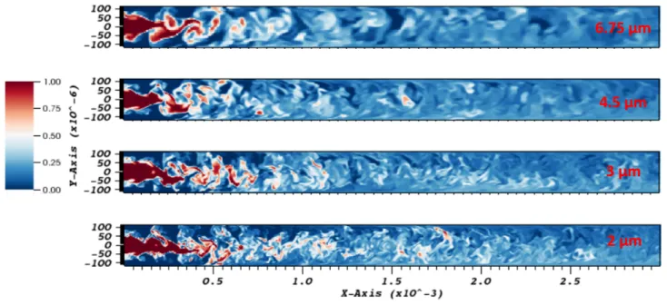
Therefore, the grid sensitivity analysis has been performed for a uniform mesh. The 4 grid sizes tested are the following: ∆x = ∆y = ∆z = 6.75 µm (mesh = 900000 cells), ∆x = ∆y = ∆z = 4.5 µm (mesh = 3 million cells), ∆x = ∆y = ∆z = 3 µm (mesh = 11 million cells) and ∆x = ∆y = ∆z = 2 µm (mesh = 37 million cells) and for a simulation with the higher mean Reynolds number (Re > 5000 of No.9 in Table 3). The Figure 6 represents the evolution of the time averaged velocity component ux and the mean mass fraction of ethanol

at the center midline of the channel. The Figure 7 represents the instantaneous ethanol mass fraction field in the plane z=0 (the longitudinal section of the channel center representing the depth along with the fluid flow direction x) for the 4 selected grid sizes. Based on these results, the velocity profiles seems to converge for grid sizes around 5 µm but for the ethanol mass fraction, the convergent length is smaller, about 3 µm. It indicates that the Kolmogorov scale is closed to 5 µm and a finer mesh is required to catch probably the Batchelor scale. This result satisfies the relation between the 2 characteristic lengths (Equation 15). Indeed, the ratio of the two characteristic length 5 µm / 3 µm is close to√Sc (≈ 1.6) estimated for the relevant conditions.

In this section, we have determined the appropriate grid size, 3 µm, close to the Kolmogorov and Batchelor microscales to well describe the turbulent mixing. This value is a good compromise between precision of resolution and CPU time of the simulations (see video 2 in supplementary data).

Figure 7: Instantaneous field of ethanol mass fraction in the plane z=0.

4.2

Simulation cases and characteristic mixing times

4.2.1

Influence of operating conditions

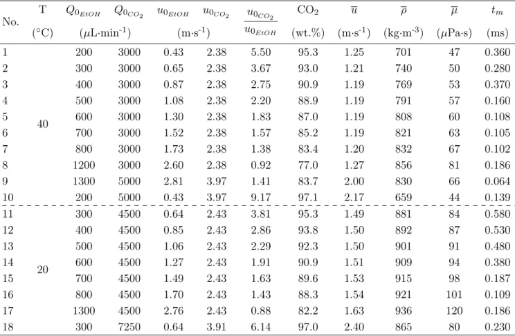
Based on the mixing conditions for µSAS processes, we have performed a set of simulation cases listed in Table 1.

Two temperatures were selected, 20 and 40◦C. The volumetric flowrates chosen for the simulations vary and are realizable experimentally in the microreactor. The mixture properties are calculated in an overall manner for the fluid mean velocity, mean density, mean viscosity and the fraction of CO2 as well as the dimensionless

numbers. The ratio of CO2 in the system is first estimated by:

CO2(wt.%) =

u0_CO2Aoutρ_CO2(T )

u0EtOHAinρEtOH(T ) + u0CO2AoutρCO2(T )

(16)

The average density ρ is then calculated by Peng-Robinson equation of state for the corresponding CO2 ratio.

The mean viscosity µ is estimated similarly by the logarithmic correlation. The fluid mean velocity is calculated by:

u = u0EtOHAinρEtOH(T ) + u0CO2AoutρCO2(T ) Achannelρ(T )

(17)

by considering the mean density ρ at the tested temperature as described just above. The segregation intensity curves are plotted with time axis related to the pure ethanol velocity in the capillary (Equation 11) and we are able to determine the characteristic mixing times tmas previously explained (examples shown in Figure 8a

and 8b). In Figure 9, we have represented the micromixing time (Equation 1) calculated locally and the evo-lution of the mean mass fraction of ethanol in the median x-y plane of the reactor. The mean mass fraction allows for locating easily the intense mixing zone. The local micromixing time values allow for comparing (and

Table 1: Conditions and fluid global properties of simulation tests with pressure fixed at 100 bar (for both ethanol and CO2 the initial velocities u0 at the capillary outlet are calculated from the fluid flowrates, considering temperatures in

the pumps and in the microchannel). The coefficient of diffusion is 1.55×10−8m2·s−1at 20◦C and 2.45×10−8m2·s−1

at 40◦C

No.

T

Q

Q

u

u

u

u

CO

u

ρ

µ

t

(

C)

(µL

·min

)

(m

·s

)

(wt.%)

(m

·s

)

(kg

·m

)

(µPa

·s) (ms)

1

40

200

3000

0.43

2.38

5.50

95.3

1.25

701

47

0.360

2

300

3000

0.65

2.38

3.67

93.0

1.21

740

50

0.280

3

400

3000

0.87

2.38

2.75

90.9

1.19

769

53

0.370

4

500

3000

1.08

2.38

2.20

88.9

1.19

791

57

0.160

5

600

3000

1.30

2.38

1.83

87.0

1.19

808

60

0.108

6

700

3000

1.52

2.38

1.57

85.2

1.19

821

63

0.105

7

800

3000

1.73

2.38

1.38

83.4

1.20

832

67

0.102

8

1200

3000

2.60

2.38

0.92

77.0

1.27

856

81

0.186

9

1300

5000

2.81

3.97

1.41

83.7

2.00

830

66

0.064

10

200

5000

0.43

3.97

9.17

97.1

2.17

659

44

0.139

11

20

300

4500

0.64

2.43

3.81

95.3

1.49

881

84

0.580

12

400

4500

0.85

2.43

2.86

93.8

1.50

892

87

0.530

13

500

4500

1.06

2.43

2.29

92.3

1.50

901

91

0.480

14

600

4500

1.27

2.43

1.91

90.9

1.51

909

94

0.380

15

700

4500

1.49

2.43

1.63

89.6

1.53

915

98

0.187

16

800

4500

1.70

2.43

1.43

88.3

1.54

921

101

0.109

17

1300

4500

2.76

2.43

0.88

82.2

1.63

936

120

0.186

18

300

7250

0.64

3.91

6.14

97.0

2.40

865

80

0.230

validating) the global value of the mixing time obtained simply by the evolution of the segregation intensity. Indeed, both values are in good agreement. The mixing times are posted in Table 3 with dimensionless numbers calculated by using the global average properties and hydraulic diameter.

(a) (b)

Figure 8: Segregation intensity curves of the simulations with characteristic mixing times of the first order system : (a). test case No.5 in Table 1 at 40◦C without time delay; (b). test case No.11 with time delay.

As a first remark and the most importantly, the mixing time is of the order of magnitude of 10−4 s. This means that the operating conditions allow for obtaining a very fast mixing with a mixing time smaller than

(a)

(b)

Figure 9: Instantaneous micromixing time fields calculated by Equation 1 in the plane z = 0 and mean time average ethanol mass fraction field: (a). test case No.5 in Table 1 at 40◦C without time delay; (b). test case No.11 with time delay.

those reported in the literature in micromixers [32]. Globally, the mixing times are comprised between 0.03 and 0.58 ms. The series of 40◦C tends to provide faster mixing due to an improved diffusion, proceeding that the segregation intensity curves fall more quickly compared to the simulations at 20◦C. In general, higher flowrates result in lower mixing times, because of a relatively higher energy dissipation rate. For a large change of the Reynolds number, the difference of mixing times is evident. Nevertheless, let us note that the global Reynolds number is also influenced by the mean mixture viscosity, which depends on the mixture composition. Therefore, for small variations of this value, the trend of mixing time is not so clear. As yet mentioned in our previous study, the effects of individual parameter are difficult to rationalize because most of parameters are correlated among them.

Table 2: Simulation conditions and tested data for microchannel and capillary dimension.

No.

Dimension

T

Q

Q

u

u

D

D

L

d

L

D

t

change

(

C)

(µL

·min

)

(m

·s

)

(µm)

(ms)

19

Channel

40

600

3000

1.30

3.09

100

170

430

170

173

199

0.250

20

2.65

430

200

131

212

0.122

21

2.29

430

260

41

219

0.132

22

3.01

400

230

53

202

0.219

23

3.77

400

170

143

190

0.180

24

3.24

400

200

100

200

0.160

25

2.99

400

260

0

197

0.226

26

2.17

450

230

102

225

0.117

27

2.73

450

170

198

206

0.340

28

2.37

450

200

150

218

0.116

29

2.03

450

260

60

229

0.126

30

Capillary

40

600

3000

2.31

2.10

75

150

430

230

90

219

0.195

31

40

600

3000

8.12

2.10

40

150

0.031

32

40

600

3000

8.12

1.73

40

105

0.035

33

40

1200

3000

4.62

2.10

75

150

0.123

34

40

1200

5000

4.62

3.50

75

150

0.098

35

20

800

3000

3.02

1.43

75

150

0.226

36

20

1600

3000

6.04

1.43

75

150

0.040

4.2.2

Influence of microchannel dimensions

As our numerical model provides precise evidences for fluid mixing in high pressure monophasic conditions, the influence on mixing time related to the microchannel dimensions can be determined to help the experimental design. To do so, several trapezoidal cross-sections have been considered in the simulation. The trapeze area can neither be too small for the capillary insertion nor too large for moderate microfluidic scales. Another constraint of the microchannel designing is due to the wet etching of silicon during the microfabrication leading to a fixed angle between the larger base and the hypotenuse of the isosceles trapezoid (58.4◦) no matter what the depth is. The tested geometries are posted in Table 2 with the test No.5 as reference for most cases (40◦C, 100 bar, ethanol flowrate at 600 µL/min and CO2 flowrate at 3000 µL/min). The characteristic length of the

microchannel is its hydraulic diameter, defined as Dh= 4A/P , with A the area and P the wet perimeter of the

trapezoidal cross-section.

For test No.19 to No.29, the cross-section changes by keeping the same capillary and the depth varies from the outer diameter (DOD) 170 µm to 260 µm. In some extreme cases, the cross-section shape is tuned to a

triangle as the depth d reaches to a high value (No.25). For test No.30 to No.36, the trapezoidal shape is the same of the simulations in Table 1 (Figure 5b) and different diameters of capillary are examined.

Based on the mixing times in Table 2, the channel depth d of 200 µm results in a slightly faster mixing. The difference is not much obvious except the cases of d = DOD at 170 µm, in which the ethanol is not

microchannel dimension influences less than the capillary diameter. The decrease of the inner diameter DOD

from 100 to 40 µm induces a tremendous increase of the ethanol velocity for the same flowrate (from 1.30 to 8.12 m/s). The ethanol rushes into the mixing zone and generates strong energy dissipation rates (2533.3 W/kg for No.31 and 2174.7 W/kg for No.32), leading to smaller mixing times.

Table 3: Results of simulation tests: global dimensionless numbers, average turbulent kinetic energy dissipation rate, micromixing times, ratio of mixing time to diffusion time and order of magnitude of the kinetic energy (CO2to ethanol).

No.

T

Re

Sc

ϵ

t

t

t

ρ

u

2

ρ

u

t

· D

D

·10

(

C)

(W

·kg

)

(ms)

1

40

4095

2.72

49.1

0.636

0.443

0.360

23.37

18.40

2

3926

2.76

81.3

0.497

0.346

0.280

10.39

14.31

3

3773

2.83

127.8

0.402

0.279

0.370

5.84

18.91

4

3633

2.92

196.5

0.329

0.229

0.160

3.74

8.18

5

3506

3.03

439.6

0.224

0.156

0.108

2.60

5.52

6

3389

3.15

509.0

0.212

0.148

0.105

1.91

5.34

7

3282

3.28

575.8

0.204

0.142

0.102

1.46

5.20

8

2932

3.86

601.6

0.216

0.150

0.186

0.65

9.52

9

5505

3.25

2429.8

0.099

0.069

0.064

1.54

3.26

10

7072

2.74

641.7

0.177

0.123

0.139

64.92

7.11

11

20

3444

6.14

66.1

0.653

0.455

0.580

16.21

18.69

12

3358

6.32

82.7

0.593

0.412

0.530

9.12

17.08

13

3277

6.51

68.6

0.660

0.459

0.480

5.83

15.47

14

3201

6.71

142.3

0.465

0.324

0.380

4.05

12.24

15

3130

6.91

301.5

0.325

0.226

0.187

2.98

6.01

16

3062

7.13

671.2

0.221

0.154

0.109

2.28

3.52

17

2778

8.30

696.7

0.234

0.163

0.186

0.86

6.00

18

5718

5.96

283.4

0.311

0.216

0.230

42.06

7.41

19

40

3720

3.03

234.0

0.307

0.214

0.250

4.38

15.45

20

3610

3.03

608.6

0.190

0.133

0.122

3.20

6.67

21

3417

3.03

438.5

0.224

0.156

0.132

2.41

6.78

22

3720

3.03

368.8

0.245

0.170

0.219

4.14

13.09

23

3950

3.03

610.5

0.190

0.132

0.180

6.50

12.17

24

3828

3.03

609.3

0.190

0.132

0.160

4.80

9.81

25

3620

3.03

353.9

0.250

0.174

0.226

4.11

14.21

26

3391

3.03

422.0

0.229

0.159

0.117

2.15

5.68

27

3574

3.03

194.1

0.337

0.235

0.340

3.41

19.71

28

3480

3.03

506.0

0.209

0.145

0.116

2.57

5.98

29

3300

3.03

359.8

0.248

0.172

0.126

1.88

5.92

30

3506

3.03

270.2

0.286

0.199

0.195

0.64

9.97

31

3506

3.03

2533.3

0.093

0.065

0.031

0.05

1.58

32

3506

3.03

2174.7

0.101

0.070

0.035

0.03

1.79

33

2932

3.86

1266.4

0.149

0.104

0.123

0.16

6.29

34

5612

3.17

1774.2

0.114

0.079

0.098

0.44

5.01

35

20

1886

5.07

206.8

0.423

0.294

0.266

0.25

8.58

36

1575

7.07

4070.3

0.113

0.078

0.040

0.06

1.29

The change of channel shape and capillary type produces fluid velocity variations, which is a key factor discussed specifically in the next part for optimizing the mixing process in the studied device configuration.

4.3

Mixing condition analysis

Since most of parameters are strongly intercorrelated to each other, it is impossible to vary only one parameter while keeping the others constant. For instance, temperature change in the channel induces fluid density variations, especially for CO2. As a consequence, for the same flowrates Q0EtOH, Q0EtOH, the initial

velocities u_{0 EtOH} u_{0 CO2} are different at the injector outlet. It is the reason why we choose to analyze a general behavior of fluid mixing. We can show in Figure 10 that the ratio between the characteristic mixing time and the diffusion time t_{dif f}(T ) = Dh2/D(T ) behaves similarly as a function of the kinetic energy ratio between CO2

and ethanol (reported in Table 3 for pure fluids before mixing). The normalization of the characteristic time by the diffusion time allows for analyzing the only influence of the inertial effects in the microchannel.

Figure 10: Evolution of the time ratio (mixing time to diffusion time) as a function of the kinetic energy ratio (CO2 to

ethanol), with 5 different regimes.

Similarly to a previous study related to two phase flows in a microfluidic device [2], we can distinguishe 5 zones of mixing behaviors. The velocity components vy and wz perpendicular to the fluid flow direction x can

also explain different regions as a function of the ratio of this kinetic energy. These two velocity components affect strongly the form of the ethanol jet at the injector outlet and they play an important role for the species dispersion, which can be observed in Figure 11 which represents the velocity vector field in y and z directions. When the ethanol energy dominates (ratio less than 0.1, No.31), it strikes into the CO2environment, engendering

velocity drop and massive energy dissipation in the mixing zone. This phenomena is less intense for a ratio between 0.1 and 1 (No.8) because the CO2 accompanies the inner fluid ethanol, flowing downstream with less

(a)

(b)

(c)

(d)

(e)

Figure 11: Instantaneous velocity vector fields in the planes of y = 0 and z = 0 for simulation tests in the mixing zone (a). No.31; (b). No.8; (c). No.7; (d). No.11; (e). No.10.

interaction in the y and z directions. As observed, compared to the former regime, the tests No.8 has less velocity dispersion at the injector outlet. The coflow mixing arrives into a local optimal region, while the energy ratio reaches about 1 to 3 (No.7). In these conditions, the CO2moves rapidly into the channel, surrounding and

shearing the ethanol, which has a shorter jet length. The interaction between two fluids creates vortices in the channel so the mixing is enhanced. When the kinetic energy of CO2 keeps increasing and the ratio steps into

a range of 3 to 20 (No.11), the CO2, with a relative high inertial force in x direction, tends to produce longer

of velocity exists in the y and z directions without velocity dispersion at the injector outlet, resulting less interaction between inner and outer fluids, and so on, involving a slower mixing than the other cases. The last zone, corresponding to an energy ratio more than 40 (No.10), represents an intense kinetic energy of CO2. The

CO2 rushes into the microchannel and blocks the inner fluid of ethanol close to the tip, leading to a very short

jet length. Consequently, these conditions provoke high dispersion (or vortices) and promote very short mixing time. This behavior has been already reported in a previous study [2].

4.4

Micromixing time & mixing performance comparison

In order to examine the robustness of our simple estimation of the characteristic mixing time, the energy dissipation rate and its average value in the mixing zone have been calculated based on Equation 13 to determine the micromixing time with Equation 1. As mentioned before, the mean energy dissipation rate ϵ has been calculated in the mixing region comprised between 0 and the length corresponding to the mixing time. The micromixing times tmE = 17.24

√

ν/ϵ and tv = 12

√

ν/ϵ are reported in Table 3, representing respectively the

engulfment micromixing time and the theoretical hydrodynamic life time of vortices. As shown in Figure 12, the turbulent mixing times obtained in the current study are in the same order of magnitude of the two models. It appears that an estimation of the mixing time has been proven as a simple and efficient method to characterize the mixing performance. It has been additionally verified the capacity of capturing the micromixing in our numerical model under tested conditions (the global Reynolds number less than 7500 in Table 3). A correlation (Equation 18) has been determined to estimate mixing time in function of the energy dissipation rate ϵ (blue line in Figure 12), which conserves the same slope (-0.5) than the laminar mixing. The coefficient 0.0034 is smaller than the laminar one 0.0075 [33], as expected, implying better mixing capacity in turbulent conditions:

tm= 0.0034· ϵ−0.5 (18)

The performance of other micromixers are collected in the literature [32,34-39] and their mixing times are mostly higher than 1 ms. It should be reminded that all experiments previously published have been performed with water at ambient pressure as a working fluid. Under our conditions in the microreactor (above the critical pressure of the mixture), a higher diffusivity and a lower viscosity are obtained for the system of CO2 and

ethanol. Our microreactor provides smaller mixing times in the order of magnitude of 0.1 ms, 10 times lower than other micromixers, probably due to the combination of turbulent conditions with supercritical fluids. The mixing times obtained from our pressure resistant microchip are plotted in Figure 13, for the same ϵ range, containing both laminar and turbulent conditions as well as laminar mixing model and turbulent correlation. As shown in Figure 13, our mixing times are close to the theoretical ones and the microreactor seems to be more efficient than those reported in the literature.

Figure 12: Mixing times acquired of turbulent mixing simulations with a correlation according to the average energy dissipation rate ϵ, compared to micromixing times and hydrodynamic life times of vortices under same conditions.

Figure 13: CO2-ethanol mixing times at 100 bar in our microreactor for both laminar and turbulent conditions and

rough comparison to other micromixers depending on the result of Falk and Commenge [32].

5

Conclusion

In this paper, we have studied the turbulent mixing in a homemade microreactor with a coflow geometry for the fluid mixture of CO2antisolvent and ethanol solvent under µSAS conditions (examined temperature at 20

and 40◦C with pressure fixed at 100 bar). By applying a coupling of a microscope and a high speed camera, we have proven that the microreactor is capable of performing fluid mixing for high pressure turbulent conditions. In

the numerical part, validated in a previous work, the grid size has been selected to capture all the mixing length scales, through direct numerical simulation (DNS). Through the CFD model, the turbulent mixing has been examined for different turbulent conditions (temperature, fluid flowrates, microchannel dimension and capillary type). The capillary dimension has a greater influence than the trapezoidal channel dimension analyzed in this study. A general fluid mixing behavior has been detected, divided into different zones based on the relationship between a time dimensionless number (the ratio of mixing time to diffusion time) and an energy dimensionless number (the ratio of CO2 kinetic energy to the ethanol’s). The micromixing time has been equally calculated,

based on the average energy dissipation rate ϵ. The results show that the mixing times derived from the first order system of the segregation intensity curve are able to well represent the turbulent mixing efficiency, which are in good agreement with the micromixing models of the literature. Compared to other micromixers, our microreactor allows for achieving mixing intensification with much smaller characteristic mixing times.

Acknowledgement

We acknowledge the French National Research Agency for it support (ANR-17-CE07-0029 - SUPERFON), the University of Bordeaux for the Ph.D. funding of the author Fan Zhang and the MCIA (Mésocentre de Calcul Intensif Aquitaine) for the HPC resources.

References

[1] F. Zhang, A. Erriguible, S. Marre, Investigating laminar mixing in high pressure microfluidic systems, Chem. Eng. Sci. 205 (2019) 25–35.

[2] F. Zhang, A. Erriguible, T. Gavoille, M.T. Timko, S. Marre, Inertia-driven jetting regimes in microfluidic coflows, Phys. Rev. Fluids 3, 092201(R) (2018).

[3] J. Baldyga, J.R. Bourne, A fluid mechanical approach to turbulent mixing and chemical reaction part II micromixing in the light of turbulence theory, Chem. Eng. Commun. 28 (1984) 243–258.

[4] J.M. Commenge, L. Falk, Villermaux-Dushman protocol for experimental characterization of micromixers, Chem. Eng. Process. 50 (2011) 979–990.

[5] J. Villermaux, L. Falk, A generalized mixing model for initial contacting of reactive fluids, Chem. Eng. Sci. 49 (1994) 5127–5140.

[6] M. Harada, Micromixing in a Continuous Flow Reactor (coalescence and redispersion models), Kyoto uni-versity, Kyoto, 1962.

[7] P. Costa, C. Trevissoi, Reactions with non-linear kinetics in partially segregated fluids, Chem. Eng. Sci. 27 (1972) 2041–2054.

[8] J. Villermaux, J.C. Devillon, Représentation de la coalescence et de la redispersion des domaines de ségréga-tion dans un fluide par un modèle d’interacségréga-tion phénométnologique, in Proceed, 2nd Inc. Symp. Chem. React. Engng, Amsterdam B (1972), pp. 1-13.

[9] J. Bałdyga, J.R. Bourne, Calculation of micromixing in inhomogeneous stirred tank reactors, Chem. Eng. Res. and Des. 66 (1988) 33–38.

[10] T. Lemenand, D. Della Valle, C. Habchi, H. Peerhossaini, Micro-mixing measurement by chemical probe in homogeneous and isotropic turbulence, Chem. Eng. J. 314 (2017) 453–465.

[11] J. Baldyga, J.R. Bourne, Comparison of the engulfment and the interaction-by-exchange- with-the-mean micromixing models, Chem. Eng. J. 45 (1990) 25–31.

[12] J. Baldyga, J.R. Bourne, Simplification of micromixing calculations. I. Derivation and application of new model, Chem. Eng. J. 42 (1989) 83–92.

[13] R. Couto, S. Chambon, C. Aymonier, E. Mignard, B. Pavageau, A. Erriguible, S. Marre, Microfluidic supercritical antisolvent continuous processing and direct spray-coating of poly-(3-hexylthiophene) nanoparticles for OFET devices, Chem. Commun. 51 (2015) 1008–1011.

[14] D. Sharma, A. Erriguible, G. Gandikota, D. Beysens, and S. Amiroudine, Vibration-induced thermal instabilities in supercritical fluids in the absence of gravity, Phys. Rev. Fluids 4, 033401 (2019).

[15] S. Amiroudine, J.-P. Caltagirone, A. Erriguible, A Lagrangian-Eulerian compressible model for the trans-critical path of near-trans-critical fluids, Int. J. Multiph. Flow 59 (2014) 15-23.

[16] A. Erriguible, S. Laugier, M. Late, P. Subra-Paternault, Effect of pressure and non-isothermal injection on re-crystallization by CO2 antisolvent: solubility measurements, simulation of mixing, and experiments, J.

Supercrit. Fluids 76 (2013) 115–125.

[17] A. Erriguible, T. Fadli, P. Subra-Paternault, A complete 3D simulation of a crystallization process induced by supercritical CO2 to predict particle size, J. Comput. Chem. Eng. 52 (2013) 1–9.

[18] P. He, A. Raghavan, A.F. Ghoniem, Impact of non-ideality on mixing of hydrocarbons and water at supercritical or near-critical conditions, J. Supercrit. Fluids 102 (2015) 50-65.

[19] P. He, A.F. Ghoniem, A sharp interface method for coupling multiphase flow, heat transfer and multicom-ponent mass transfer with interphase diffusion, J. Comput. Phys. 332 (2017) 316-332.

[20] P. He, A.F. Ghoniem, Phase separation during mixing of partially miscible fluids under near-critical and supercritical conditions, and the phenomenon of uphill diffusion, J. Supercrit. Fluids 135 (2018) 105-119. [21] F.A. Sánchez, P. He, A.F. Ghoniem, S. Pereda, Modeling hydrocarbon droplet dissolution in near-critical or supercritical water using GCA-EOS and non-ideal diffusional driving force in binary mixtures, J. Supercrit. Fluids 146 (2019) 1-14.

[22] Y. Maeta, M. Ota, Y. Sato, R.L. Smith, H. Inomata, Measurements of vapor–liquid equilibrium in both binary carbon dioxide–ethanol and ternary carbon dioxide–ethanol–water systems with a newly developed flow-type apparatus, Fluid Phase Equilib. 405 (2015) 96–100.

[23] NIST (National Institute of Standards and Technology). <http://www.webbook.nist.gov/chemistry/>. [24] W. Hayduk, B.S. Minhas, Correlations for prediction of molecular diffusivities in liquids, The Canadian J. Chemical Engineering 60 (1982) 295–299.

[25] T. Fadli, A. Erriguible, S. Laugier, P. Subra-Paternault, Simulation of heat and mass transfer of CO2

–solvent mixtures in miscible conditions: isothermal and non-isothermal mixing, J. Supercrit. Fluids 52 (2010) 193–202.

[26] P.L. Roe, Characteristic-based schemes for the Euler equations, Annu Rev Fluid Mech 18 (1986) 337–365. [27] R.D. Falgout, U.M. Yang, hypre: A library of high performance preconditioners. In: Proceedings of the international conference on computational science. Springer; 2002. p. 632–41.

[28] P. Danckwerts, The effect of incomplete mixing on homogeneous reactions, Chem. Eng. Sci. 8 (1958) 93–102.

[29] G. Scholz, F. Scholz, First-order differential equations in chemistry. ChemTexts, 2015, 1, (1), p. 1. [30] P. Guichardon, L. Falk, 2000. Characterisation of micromixing efficiency by the iodide–iodate reaction system. Part I. Experimental procedure, Chem. Eng. Sci. 55, 4233–4243.

[31] L. Metzger, Process Simulation of Technical Precipitation Processes The Influence of Mixing, PhD thesis Karlsruhe Institute of Technology 2017.

[32] L. Falk, J.-M. Commenge, Performance comparison of micromixers, Chem. Eng. Sci. 65 (2010) 405–411. [33] J. Baldyga, J.R. Bourne, Encyclopedia of Fluid Mechanics, Flow Phenomena and Measurement 1 (1986), Gulf Pub Co.

[34] S. Panić, S. Loebbecke, T. Tuercke, J. Antes, D. Bošković, Experimental approaches to a better under-standing of mixing performance of microfluidic devices, Chem. Eng. J. 101 (2004) 409–419.

[35] N. Kockmann, T. Kiefer, M. Engler, P. Woias, Convective mixing and chemical reactions in microchannels with high flow rates, Sens. Actuators B 117 (2006) 495–508.

[36] N. Aoki, K. Mae, Effects of channel geometry on mixing performance of micromixers using collision of fluid segments, Chem. Eng. J. 118 (2006) 189–197.

[37] R. Keoschkerjan, M. Richter, D. Boskovic, F. Schnürer, S. Löbbecke, Novel multifunctional microreaction unit for chemical engineering, Chem. Eng. J. 101 (2004) 469–475.

[38] M.A. Schneider, T. Maeder, P. Ryser, F. Stoessel, A microreactor-based system for the study of fast exothermic reactions in liquid phase: characterization of the system, Chem. Eng. J. 101 (2004) 241–250. [39] Y. Men, V. Hessel, P. Löb, H. Löwe, B. Werner, T. Baier, Determination of the segregation index to sense the mixing quality of pilot-and production-scale microstructured mixers, Chem. Eng. Res. Des. 85 (5) (2007) 605–611.