HAL Id: hal-00639663
https://hal.archives-ouvertes.fr/hal-00639663
Submitted on 9 Nov 2011
HAL is a multi-disciplinary open access
archive for the deposit and dissemination of
sci-entific research documents, whether they are
pub-lished or not. The documents may come from
teaching and research institutions in France or
abroad, or from public or private research centers.
L’archive ouverte pluridisciplinaire HAL, est
destinée au dépôt et à la diffusion de documents
scientifiques de niveau recherche, publiés ou non,
émanant des établissements d’enseignement et de
recherche français ou étrangers, des laboratoires
publics ou privés.
LNA: Fast Protein Classification Using A Laplacian
Characterization of Tertiary Structure
Nicolas Bonnel, Pierre-François Marteau
To cite this version:
Nicolas Bonnel, Pierre-François Marteau.
LNA: Fast Protein Classification Using A Laplacian
Characterization of Tertiary Structure. IEEE/ACM Transactions on Computational Biology and
Bioinformatics, Institute of Electrical and Electronics Engineers, 2012, 9 Issue: 5, pp.1451 - 1458.
�10.1109/TCBB.2012.64�. �hal-00639663�
LNA: Fast Protein Classification Using A Laplacian
Characterization of Tertiary Structure
Nicolas Bonnel and Pierre-Francois Marteau
IRISA-UBS, Universit´
e de Bretagne Sud, France
[email protected], [email protected]
November 9, 2011
Abstract
1
Motivation:
In the last two decades, a lot of protein 3D shapes have been discovered, characterized and made avail-able thanks to the Protein Data Bank (PDB), that is nevertheless growing very quickly. New scalable methods are thus urgently required to search through the PDB efficiently.
2
Results:
We present in this paper an approach entitled LNA (Laplacian Norm Alignment) that performs struc-tural comparison of two proteins with dynamic pro-gramming algorithms. This is achieved by charac-terizing each residue in the protein with scalar fea-tures. The feature values are calculated using a Laplacian operator applied on the graph correspond-ing to the adjacency matrix of the residues. The weighted Laplacian operator we use estimates at var-ious scales local deformations of the topology where each residue is located. On some benchmarks widely shared by the community we obtain qualitatively sim-ilar results compared to other competing approaches, but with an algorithm one or two order of magni-tudes faster. 180,000 protein comparisons can be done within 1 seconds with a single recent GPU, which makes our algorithm very scalable and suitable for real-time database querying across the Web.
3
Introduction
Proteins are made of a sequence of amino acids (residues) that folds in a 3 dimensional structure.
Proteins having similar functional properties may have a very different primary structure, but they usu-ally share similar tertiary structures. During the past two decades, a lot of tertiary structures have been discovered, and 3D fold protein data banks such as PDB [4] are quickly growing (PDB holds 79000 pro-tein files as of November 2011). It is therefore crucial to be able to efficiently search through this database. Best methods designed to compare or match pro-tein 3D structures involve heavy computations. [16] compares Cαdistance matrices, [30] extendedly com-bines aligned fragment pairs based on local geometry, [18] compares lists of feature of primary, secondary and tertiary structures, [34, 28] maximize the TM-score which is independent of protein lengths con-trary to the Root Mean Square Deviation (RMSD: [19]). [35] compares intra-molecular residue-residue relationship. [14, 22] first align secondary struc-ture elements (SSE) and then refine the alignment to residue level. Some approaches are based on con-tact maps matching which is though to be NP-hard as descibed by [15]: [6, 3, 12]. [27] uses double dy-namic programming on vector of Cβdistances and is used to build the CATH [9] classification.
On the other hand, a few methods are a lot faster, nevertheless at the cost of results quality. [33] en-hances BLAST [2] by using a structural alphabet and corresponding substitution matrix. [23, 24] enhance BLAST using an alphabet corresponding to residue positions in the Ramachandran plot [29]. [7] char-acterizes proteins as sequences of α angles (dihedral angle between four consecutive α carbons) and com-pares them by searching common fixed length pat-terns. [21] performs a global alignment of structural signatures.
We present in this paper a novel way for describing protein 3D structures. While Cartesian coordinates
of a residue are dependent upon a reference coordi-nate system and only give information about its loca-tion, differential coordinates carry information about the local topology and the orientation of local struc-tural details. We use the norm of Laplacian coordi-nates of residues at different scales to encode a se-quence of multivariate local deformation descriptors. The norm of the Laplacian coordinates presents the great advantage to be invariant to translation and rotation.
The Laplacian operator have been used in various methods, mainly for 3D computer vision and 3D mod-eling. [25] performs articulated shape matching. [11] uses this operator to smoothen, enhance or check the quality of triangular meshes.
Dynamic programming algorithms can then be used to match these multivariate descriptor sequences and achieve similar classification or clustering results compared to other approaches. These dynamic pro-gramming algorithms in O(n2) time complexity re-quire few memory and can be efficiently implemented on Graphical Processing Unit (GPU) for an even faster computation time. This allows to compare one protein structure against 180,000 others within a sec-ond time span.
In the following, we describe how we compute the Laplacian coordinates of residues and their norm. We then present two dynamic programming algorithms derived from [26] and [31] for global and local align-ment respectively and compare our approach with state of the art methods on two protein datasets known to be difficult to categorize. We show that our approach outperforms the fastest know methods and provides qualitatively similar results than most of the best known approaches, with algorithms one or two order of magnitude faster.
4
Method and algorithm
Our method, called Laplacian Norm Alignment (LNA), characterizes proteins as a multi-dimensional sequence of quantity of deformation at different scales of the local space in which residues are embedded. More precisely, the discrete Laplace operator (dis-crete Laplacian) is used to measure the divergence of the gradient of residue positions in a graph that describes a protein weighted adjacency map. Lapla-cian coordinates of residues are resilient to translation but not to rotation. This limitation is overcome by only keeping for each residue the Euclidean norm of its Laplacian coordinates that is indeed invariant to
rotation.
The tertiary structure of a protein is usually en-coded as sequence of 3D Cartesian space coordinates for each atom of each amino acid. We simplify this sequence by only keeping carbon alpha (Cα) 3D po-sitions for each residue.
4.1
Computation of the Laplacian
co-ordinates of each residue
A protein P of length n is defined by a sequence of 3D coordinates p1, p2, . . . , pn. Let ΩP(σ) be the weighted adjacency matrix of an undirected graph with one node per residue for the protein P . The weight ΩP
ij(σ) of each edge eij for 1 ≤ i, j ≤ n is computed using a Gaussian kernel: ΩPij(σ) = e−kpi−pj k 2 σ2 if |i − j| > 1
0 otherwise and in this case there is no edge (1) Let the diagonal matrix DP(σ) be defined as:
DP ii(σ) = X j ΩP ij(σ) (2)
The discrete Laplace operator LP(σ) of the protein P is given by:
LP(σ) = I − DP(σ)−1
ΩP(σ) (3) By applying this operator to the vector of the residue 3D Cartesian positions, we obtain a vector of 3D Laplacian coordinates for each residue. Finally, we build a sequence eP(σ) = ep1(σ), ep2(σ), . . . , epn(σ) of Euclidean norms of the Laplacian coordinates for each residue, as shown on figure 1.
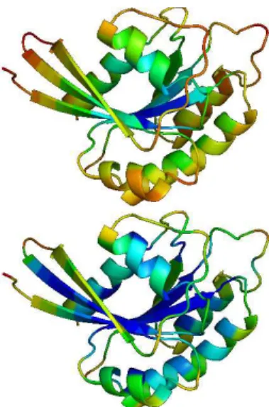
Since we use a Gaussian kernel, the norm of the Laplacian coordinates is usually higher in the periph-ery of the protein than in the center, as shown on figure 2(b). Hence, beta sheets generate a lowly de-formed surface, the norm of Laplacian coordinates of their residues is quite low. A contrario coils can have a high norm of Laplacian coordinates corresponding to their residues if they are found in the periphery of the protein. Alpha helices rarely go through the center of the protein: for each alpha helix, a ’side’ is near the center of the protein and the other near the periphery. Consequently, consecutive residues in the chain have a norm of their Laplacian coordinates that vary: thus, alpha helices correspond to a saw-tooth shape as shown on figure 2(a).
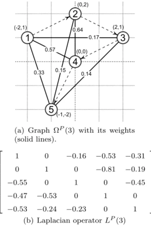
1 2 3 4 5 (-2,1) (0,2) (2,1) (0,0) (-1,-2) 0.17 0.57 0.33 0.64 0.15 0.14 (a) Graph ΩP
(3) with its weights (solid lines). 1 0 −0.16 −0.53 −0.31 0 1 0 −0.81 −0.19 −0.55 0 1 0 −0.45 −0.47 −0.53 0 1 0 −0.53 −0.24 −0.23 0 1 (b) Laplacian operator LP(3)
Figure 1: Example of Laplacian computation for a protein P in 2D with σ = 3 and k = 1. The sequence of norm of Laplacian coordinates is eP = eP(3) = 2.48, 2.39, 3.80, 1.80, 3.26.
4.2
Multi-dimensional
characteriza-tion of residues
The σ parameter in the Gaussian kernel can be tuned such as to correspond to either a more local or more global description of the protein for each residue. A low σ implies that only the closest residues will be taken into account into the computation of the Lapla-cian coordinates of residues. On the other hand, a high σ implies that all other residues in the pro-tein will be taken into account into the computation, the difference of contribution between close and far residues being lower.
The Van Der Walls radius of atoms implies that sigma should be above 2˚A, and the average size of proteins implies that it should be bellow 50˚A. As in-formation on residue positions is lost when only keep-ing the norm of Laplacian coordinates, this geomet-ric description suffers a loss of information that can reduce the discriminating capability of the alignment algorithms. This limitation can be overcome by char-acterizing the local topology in which each residue is embedded at different scales, while varying parame-ter σ. For instance, residues can be characparame-terized by
2 norms of Laplacian coordinates: one corresponding to coordinates computed with σ < 10˚A (local de-scription) and the other with σ > 20˚A (more global description).
Hence a protein P of length n can be characterized by a sequence eP = ep1,ep2, . . . ,pen of k-dimensional vectors defined as follows:
e
pi= [epi(σ1), epi(σ2), . . . , epi(σk)], 1 ≤ i ≤ n (4) where σ1, σ2, . . . , σk are all in [2; 50].
4.3
Sequence comparison
We propose 2 dynamic programming approaches for global and local comparison of proteins. Given two sequences ePand eQof respective length m and n, both approaches perform computations in O(m.n) time, and use k-dimensional vectors for the characteriza-tion of residues.
More precisely, the similarity is computed by com-paring segments of the multivariate sequence that de-scribe each protein. Let τ (epi,qej) be the dissimilarity between the i-th segment (i.e. i-1-th and i-th values) of eP and j-th segment of eQ, and defined as follows:
τ(epi,eqj) = k X t=1 ( |epi(σt) − eqj(σt)| + |epi−1(σt) − eqj−1(σt)|+ 3.|(epi(σt) − epi−1(σt)) − (eqj(σt) − eqj−1(σt))|
(5) The constant value 3 has been empirically de-termined during preliminary experiments as a good trade-off allowing to weight the contributions of the differences between segment extremities and the dif-ferences between segment slopes.
4.3.1 Global comparison
The global similarity LNAN W k between two se-quences eP and eQ with respective lengths m and n is evaluated using a dynamic programming algorithm derived from [26].
LN AN W k( eP , eQ) = p S(epm,qen)
(m − 1).(n − 1) (6) and recursively defined as follows:
S(epi,qej) = max S(epi−1,eqj) S(epi−1,eqj−1) + e−ν.τ ( epi,eqj) S(epi,qej−1) (7)
(a) Euclidean norms of the 3D Laplacian coordinates com-puted for each residue for two didderent σ values and super-imposed secondary structure.
(b) Low values are coded in blue while high values are coded in red. This figure was made with PyMol [10].
Figure 2: Protein SCOP/Astral id d3raba . Norm of Laplacian coordinates with σ = 20 (top) and σ = 4 (bottom).
with the following initial conditions:
S(ep0,qej) = S(epi,eq0) = S(ep0,eq0) = 0
The scoring function e−ν.τ ( epi,eqj) ranges in [0 .. 1]
and is maximal when segment extremities have the same Laplacian coordinates norms in all k dimen-sions. The constant gap penalty is set to 0 so that the similarity measure we propose is normalized in [0 .. 1]. This property can be very useful to per-form fast filtering for quick searching or large scale database clustering. Fast filtering can be achieved by only comparing sequences length.
4.3.2 Local comparison
For local comparison, the computation of τ (epi,eqj) is performed using normalized Laplacian norm se-quences: all epiand eqj values are divided by the aver-age of the sequence eP and eQrespectively, so that the average of each Laplacian norm sequence is 1. The lo-cal similarity LNASW kbetween two sequences ePand
e
Qwith respective lengths m and n is evaluated using a dynamic programming algorithm derived from [31].
LN ASW k( eP , eQ) = max{S(epi,qej), 1 ≤ i ≤ m, 1 ≤ j ≤ n} (8) and recursively defined as follows:
S(epi,qej) = max S(epi−1,eqj) + g S(epi−1,eqj−1) + 1 − ν.τ (epi,eqj) S(epi,qej−1) + g 0 (9) with the following initial conditions:
S(ep0,eqj) = S(epi,q0e) = S(ep0,q0) = 0e
Contrary to LNAN W k, this measure is not normal-ized and ranges in [0 .. min(m, n)] with a negative gap penalty value.
5
Results and discussion
Dynamic programming algorithms require low mem-ory usage. Both LNAN W k and LNASW k algorithms are implemented on GPU using the OpenCL language [20]. Experiments are performed on a Nvidia Tesla
M2050 GPU. We first use a subset of SCOP [17] to determines optimal parameters. We then evalu-ate our approach on ranking and classification tasks against two different datasets: COPS [13] and pro-teus300 [3, 12]. We also measure speed performance on the whole PDB database to see how our approach scales when applied to real databases.
5.1
Optimization of the parameter
values
Both dynamic programming algorithms we propose require to adjust few parameters. We determine opti-mal sets of parameter values using a subset of SCOP downloaded on the Astral compendium website [8]. From the the 40% ID filtered subset of SCOP 1.75, among 640 families having at least 4 members, we se-lect at random 4 proteins from each family . We then build 4 subsets (one protein from each family in each subset) and perform a 4-fold cross-validation to op-timize the set of parameters. For each query set, we record the top 3 returned results and check whether they belong to the same family of the query or not. Thus, the best possible score is 3 × 4 × 640 = 7680.
Parameter values are determined for LNAN W kand LNASW k with k ∈ {1, 2}. We also performed tests with higher values for k. However, results tend to decrease in quality as a higher number of dimension is used and computational time increases.
Method LNASW 1 LNASW 2 LNANW 1 LNANW 2 Gap -0.53 -0.5 NA NA σ1 5.7 5.0 6.1 5.4 σ2 NA 14.5 NA 14.3 ν 0.67 0.41 0.24 0.15 Score 5468 5757 5333 5523 Score (%) 71.20 74.96 69.44 71.91 Time (sec) 74 82 86 98
Table 1: Optimal parameter values found using 2560 proteins from the 40% ID filtered subset of SCOP 1.75.
Table 1 shows optimal parameter values found. For the remainder of this paper, our approaches are pa-rameterized with these values. We also reported the time used by the GPU to compute the 4,915,200 com-parisons. LNASW2, which obtains the best results, performs about 60,000 protein comparisons per sec-ond. For best performances, we recommend using k= 2.
Figure 3 plots the ROC curves for LNA approaches. The false positive rate starts to increase when about 75 % of correct answers is returned.
Table 2 shows the precision obtained according to
Figure 3: ROC curves for LNA on a 2560 proteins subset of the 40% ID filtered subset of SCOP 1.75.
Precision LNASW 1 LNASW 2 LNANW 1 LNANW 2 1 124 150 0.67 0.59 0.95 50 51 0.56 0.45 0.9 43 42 0.54 0.43 0.8 37 35 0.52 0.40
Table 2: Precision according to LNA score obtained on a 2560 proteins subset of the 40% ID filtered subset of SCOP 1.75.
LNA score returned. For instance, if the comparison of two proteins using LNAN W2returns a score of 0.45, then there is 95 % chance that these two proteins belong to the same SCOP family.
5.2
COPS
The COPS benchmark [13] is built upon the COPS classification performed by [32]. This benchmark contains 176 queries, and for each query there is 6 true positives and 1050 true negatives. We use this benchmark to compare alignment methods by plot-ting ROC curves. We compare our approach against FAST [35], GOSSIP [21] and Yakuza [7]. We use the default parameters for FAST and Yakuza. For GOSSIP, we use an accuracy of 10 and two similarity values (0.6 and 0.7).
Figure 4 plots the ROC curve for each approach. FAST is the best approach for this benchmark and GOSSIP is the worst. Our approach is above Yakuza using the local alignment method and bellow it with the global one.
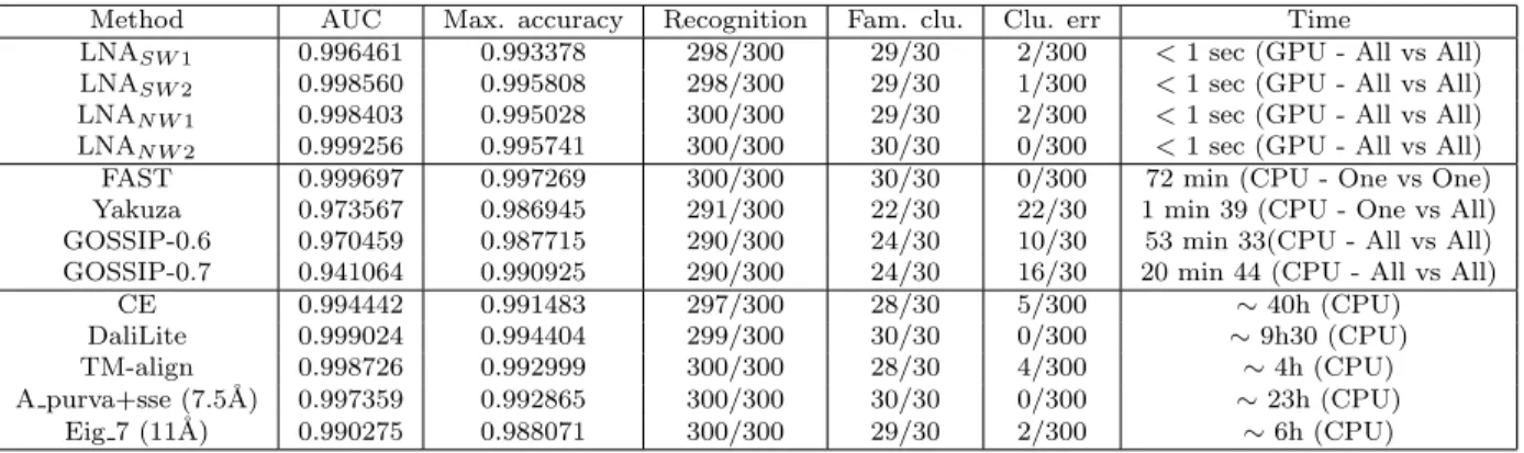
Method AUC Max. accuracy Recognition Fam. clu. Clu. err Time
LNASW 1 0.996461 0.993378 298/300 29/30 2/300 <1 sec (GPU - All vs All) LNASW 2 0.998560 0.995808 298/300 29/30 1/300 <1 sec (GPU - All vs All) LNAN W 1 0.998403 0.995028 300/300 29/30 2/300 <1 sec (GPU - All vs All) LNAN W 2 0.999256 0.995741 300/300 30/30 0/300 <1 sec (GPU - All vs All) FAST 0.999697 0.997269 300/300 30/30 0/300 72 min (CPU - One vs One) Yakuza 0.973567 0.986945 291/300 22/30 22/30 1 min 39 (CPU - One vs All) GOSSIP-0.6 0.970459 0.987715 290/300 24/30 10/30 53 min 33(CPU - All vs All) GOSSIP-0.7 0.941064 0.990925 290/300 24/30 16/30 20 min 44 (CPU - All vs All)
CE 0.994442 0.991483 297/300 28/30 5/300 ∼ 40h (CPU) DaliLite 0.999024 0.994404 299/300 30/30 0/300 ∼ 9h30 (CPU) TM-align 0.998726 0.992999 300/300 28/30 4/300 ∼ 4h (CPU) A purva+sse (7.5˚A) 0.997359 0.992865 300/300 30/30 0/300 ∼ 23h (CPU) Eig 7 (11˚A) 0.990275 0.988071 300/300 29/30 2/300 ∼ 6h (CPU)
Table 3: Ranking, classification, clustering and speed performances results for the proteus 300 dataset.
Figure 4: ROC curves for the COPS benchmark.
5.3
Proteus300
The proteus300 dataset was first used in [3] and later in [12]. It contains 300 protein domains evenly dis-tributed across 30 SCOP families (27 super-families and 24 folds). The number of residues in the proteins ranges from 64 to 455. Protein length are quite ho-mogeneous inside families. Contrary to COPS bench-mark, global alignment methods should perform well on this dataset.
We measure classification, Area Under the ROC Curve (AUC) [5], maximum accuracy, clustering and speed performances. We compare our approach against the same methods than in section 5.2: [35, 21, 7] using the same settings. We also report re-sults from [12]. Rere-sults are summarized in table 3. AUC and accuracy measures were computed using the ROCR package [1].
For each protein, we compute its similarity score
with all other proteins and assign the family of the most similar protein in the dataset (Nearest Neigh-bor rule). We then measure the number of correctly assigned families for the whole dataset. Yakuza and GOSSIP obtain the worst results. All other presented approaches reach similar classification performances (table 3, col. 4): all approaches have at most 3 errors on the 300 protein domains and 6 of them (LNAN W1, LNAN W2, FAST, TM-align, A purva+sse and Eig 7) have no error.
The similarity matrix is also used to compute AUC and accuracy (3, col. 2-3)) measures. Our approach has comparable results with respect to other meth-ods. Again, FAST obtains the best results, while we rank second on AUC criterion with the global align-ment method and second on maximum accuracy cri-terion with the local alignment method.
We measure clustering performances at family level with the Un-weighted Pair Group Method with Arithmetic Mean (UPGMA) algorithm (3, col. 5-6)). Our approach achieves comparable results with state of the art methods. The global alignment method performs slightly better than the local one, LNAN W2 achieving a perfect classification.
Finally we give the computational time required to compute the similarity matrix between all 300 proteins. Experiments were run on a 2 GHz Intel Xeon and 8GB RAM for [35, 21, 7]. For other ap-proaches, we used results reported in [12] and ob-tained with a 2.8 GHz CPU Intel Pentium and 1GB RAM. One vs One means both proteins are prepro-cessed for each comparison. One vs All means a query is preprocessed and compared against a pre-processed database. All vs All means all proteins of a preprocessed database are compared between them-selves.
Even with a 100x gain compared to CPU (which is usually the best performances obtained by porting an algorithm to GPU), we can see that our approach is one or two order of magnitude faster compared to other approaches, while achieving very good results. These performances are due to the O(n2) time com-plexity of alignment algorithms that is used for the matching of pair of proteins.
We believe Yakuza could be as fast as our approach if ported on GPU, however we obtain better ranking and classification performances with our approach on both tested datasets. On both COPS and Proteus datasets, FAST achieves the best results but ranks fourth for the speed. On the other hand, LNA ranks second for the quality of results but is the fastest method.
5.4
Experiment on the whole PDB
database
As of November 2011 the Protein Data Bank contains about 79,000 protein files. By only keeping sequences with a minimum length of 30, we obtain 179,094 ter-tiary structures of proteins, with an average length of 247. We measure in this experiment how our ap-proach performs for a real scale problem. We mea-sure speed for LNASW2 and LNAN W2. We also test various score acceptation threshold for LNAN W2 to measure fast filtering performances.
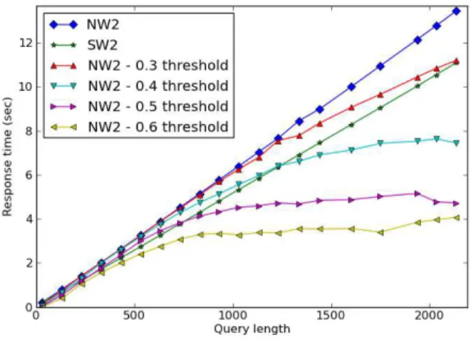
Figure 5: Response time for one query against the whole PDB database.
Figure 5 shows the response time according to query length. As shown on previous experiments, LNAN W2 is the slowest alignment method proposed. For all approaches, the average response time for a
200 residue length query is around 1 second, which is very suitable for a real-time Web service. Fast fil-tering allowed by the normalized LNAN W2alignment method is very interesting when looking for high pre-cision. It allows a speedup up to 3 times for very long protein queries. For a 230 residue length query, the reported speedup is around 34 % with a 0.6 score acceptation threshold.
6
Conclusions
We have proposed in this paper an approach for speeding up computation of protein structure similar-ity. We have presented an approach that compresses 3D information into meaningful 1D or 2D informa-tion. Our algorithm obtains similar results as state of the art methods, as shown by experiments per-formed using various datasets. But the key advan-tage of our approach is its speed. Our algorithm is one or 2 order of magnitude faster than existing meth-ods: 180,000 protein comparisons can be done within 1 seconds with a single recent GPU, which makes our algorithm very scalable and suitable for real-time database querying across the Web. We plan to look if our approach could be improved by using primary structure information. We are also looking forward how to realize multiple sequence alignment.
7
Acknowledgement
We thanks the French Ministry of Research,the Brit-tany Region, the General Council of Morbihan and the European Regional Development Fund.
References
[1] ROCR: visualizing classifier performance in R. Bioinfor-matics, 21(20):3940–3941, October 2005.
[2] Stephen F. Altschul, Thomas L. Madden, Alejandro A. Schffer, Jinghui Zhang, Zheng Zhang, Webb Miller, and David J. Lipman. Gapped blast and psiblast: a new gen-eration of protein database search programs. NUCLEIC ACIDS RESEARCH, 25(17):3389–3402, 1997.
[3] Rumen Andonov, Nicola Yanev, and No¨el Malod-Dognin. An efficient lagrangian relaxation for the contact map overlap problem. In Proceedings of the 8th international workshop on Algorithms in Bioinformatics, WABI ’08, pages 162–173, Berlin, Heidelberg, 2008. Springer-Verlag. [4] Helen M. Berman, John Westbrook, Zukang Feng, Gary Gilliland, T. N. Bhat, Helge Weissig, Ilya N. Shindyalov, and Philip E. Bourne. The protein data bank. Nucleic Acids Res, 28:235–242, 2000.
[5] Andrew P. Bradley. The use of the area under the roc curve in the evaluation of machine learning algorithms. Pattern Recognition, 30(7):1145 – 1159, 1997.
[6] A. Caprara, R. Carr, S. Istrail, G. Lancia, and B. Walenz. 1001 optimal PDB structure alignments: integer program-ming methods for finding the maximum contact map over-lap. J Comput Biol, 11(1):27–52, 2004.
[7] M. Carpentier, S. Brouillet, and J. Pothier. Yakusa: a fast structural database scanning method. Proteins, 61(1):137–51, 2005.
[8] J. M. Chandonia, G. Hon, N. S. Walker, L. Lo Conte, P. Koehl, M. Levitt, and S. E. Brenner. The ASTRAL compendium in 2004. Nucleic acids research, 32(Database issue):D189–D192, January 2004.
[9] Alison L. Cuff, Ian Sillitoe, Tony Lewis, Andrew B. Clegg, Robert Rentzsch, Nicholas Furnham, Marialuisa Pellegrini-Calace, David Jones, Janet Thornton, and Christine A. Orengo. Extending CATH: increasing cover-age of the protein structure universe and linking structure with function. Nucleic Acids Research, 39(suppl 1):D420– D426, January 2011.
[10] W. L. Delano. The PyMOL Molecular Graphics System. http://www.pymol.org, 2002.
[11] M. Desbrun, M. Meyer, P. Schr¨oder, and A. H. Barr. Dis-crete Differential-Geometry Operators for Triangulated 2-Manifolds. VisMath, ’02:35–57, 2002.
[12] Pietro Di Lena, Piero Fariselli, Luciano Margara, Marco Vassura, and Rita Casadio. Fast overlapping of protein contact maps by alignment of eigenvectors. Bioinformat-ics, 26:2250–2258, September 2010.
[13] Karl Frank, Markus Gruber, and Manfred J. Sippl. COPS benchmark: interactive analysis of database search meth-ods. Bioinformatics (Oxford, England), 26(4):574–575, February 2010.
[14] J. F. Gibrat, T. Madej, and S. H. Bryant. Surprising similarities in structure comparison. Current opinion in structural biology, 6(3):377–385, June 1996.
[15] Deborah Goldman, Sorin Istrail, and Christos H. Pa-padimitriou. Algorithmic aspects of protein structure sim-ilarity. In IEEE Symposium on Foundations of Computer Science, pages 512–522, 1999.
[16] L. Holm and C. Sander. Protein structure comparison by alignment of distance matrices. Journal of molecular biology, 233(1):123–138, September 1993.
[17] TJ Hubbard, B Ailey, SE Brenner, AG Murzin, and C Chothia. Scop: a structural classification of proteins database. Nucl. Acids Res., 27(1):254–256, 1999. [18] Jongsun Jung and Byungkook Lee. Protein structure
alignment using environmental profiles. Protein Engineer-ing, 13(8):535–543, 2000.
[19] W. Kabsch. A Solution for the Best Rotation to Relate Two Sets of Vectors. Acta Crystallographica, 32:922–923, 1976.
[20] Khronos Group. The OpenCL Specification, September 2010.
[21] Ilona Kifer, Ruth Nussinov, and Haim J. Wolfson. Gossip: a method for fast and accurate global alignment of protein structures. Bioinformatics, 27(7):925–932, 2011.
[22] E. Krissinel and K. Henrick. Secondary-structure match-ing (SSM), a new tool for fast protein structure alignment in three dimensions. Acta Crystallographica Section D, 60(12 Part 1):2256–2268, Dec 2004.
[23] W. Lo, P. Huang, C. Chang, and P. Lyu. Protein struc-tural similarity search by ramachandran codes. BMC Bioinformatics, 8(1):307, 2007.
[24] W. Lo, C. Lee, C. Lee, and P. Lyu. isarst: an integrated sarst web server for rapid protein structural similarity searches. Nucleic Acids Res, 2009.
[25] Diana Mateus, Radu Horaud, David Knossow, Fabio Cuz-zolin, and Edmond Boyer. Articulated shape matching us-ing laplacian eigenfunctions and unsupervised point reg-istration, 2008.
[26] Saul B. Needleman and Christian D. Wunsch. A gen-eral method applicable to the search for similarities in the amino acid sequence of two proteins. Journal of Molecular Biology, 48(3):443 – 453, 1970.
[27] C. A. Orengo and W. R. Taylor. Ssap: Sequential struc-ture alignment program for protein strucstruc-ture comparison. 1996.
[28] Shashi Bhushan Pandit and Jeffrey Skolnick. Fr-tm-align: a new protein structural alignment method based on frag-ment alignfrag-ments and the tm-score. BMC Bioinformatics, 9, 2008.
[29] G. N. Ramachandran and V. Sasisekharan. Conformation of Polypeptides and Proteins, volume 23 of Advances in Protein Chemistry, pages 283–437. 1968.
[30] Ilya N. Shindyalov and Philip E. Bourne. Protein struc-ture alignment by incremental combinatorial extension (ce) of the optimal path. 1998.
[31] T. F. Smith and M. S. Waterman. Identification of com-mon molecular subsequences, 1981.
[32] Stefan J. Suhrer, Markus Wiederstein, Markus Gruber, and Manfred J. Sippl. COPSa novel workbench for explo-rations in fold space. Nucleic Acids Research, 37(suppl 2):W539–W544, July 2009.
[33] J. Yang and C. Tung. Protein structure database search and evolutionary classification. Nucleic Acids Res, 34(13):3646–59, 2006.
[34] Yang Zhang and Jeffrey Skolnick. Tm-align: a protein structure alignment algorithm based on the tm-score. Nu-cleic Acids Research, 33:2302–2309, 2005.
[35] Jianhua Zhu and Zhiping Weng. Fast: a novel protein structure alignment algorithm. Proteins, 58(3):618–27, 2005.