Ecological constraints coupled with deep-time habitat dynamics predict the latitudinal diversity gradient in reef fishes

Subject Category:

Evolution

Subject Areas:

evolution, computational biology, ecology

Keywords:

diversification, latitudinal diversity gradient,

mechanistic model, palaeohabitat, reef fish

Author for correspondence:

Théo Gaboriau

e-mail: theo.gaboriau@unil.ch

†

_{These authors shared senior authorship.}

Ecological constraints coupled with

deep-time habitat dynamics predict the

latitudinal diversity gradient in reef fishes

Théo Gaboriau

_{, Camille Albouy}

_{, Patrice Descombes}

_{, David Mouillot}

_,

Loïc Pellissier

_{and Fabien Leprieur}

1_{MARBEC, Université de Montpellier, CNRS, Ifremer, IRD, Montpellier, France}

2_{Department of Computational Biology, University of Lausanne, Rue du Bugnon 27, 1011 Lausanne, Switzerland}

3_{IFREMER, Unité Ecologie et Modèles pour l’Halieutique, Rue de l’Ile d’Yeu, BP21105, 44311 Nantes cedex 3, France}

4_{Unit of Ecology and Evolution, University of Fribourg, Chemin du Musée 10, 1700 Fribourg, Switzerland}

5_{Swiss Federal Research Institute WSL, 8903 Birmensdorf, Switzerland}

6_{Landscape Ecology, Institute of Terrestrial Ecosystems, ETH Zürich, 8044 Zürich, Switzerland}

7_{Australian Research Council Centre of Excellence for Coral Reef Studies, James Cook University, Townsville,}

Queensland 4811, Australia

8_{Institut Universitaire de France, Paris, France}

TG, 0000-0001-7530-2204; LP, 0000-0002-2289-8259

We develop a spatially explicit model of diversification based on palaeohabi-tat to explore the predictions of four major hypotheses potentially explaining

the latitudinal diversity gradient (LDG), namely, the ‘time-area’, ‘tropical

niche conservatism’, ‘ecological limits’ and ‘evolutionary speed’ hypotheses. We compare simulation outputs to observed diversity gradients in the global reef fish fauna. Our simulations show that these hypotheses are non-mutually exclusive and that their relative influence depends on the time scale considered. Simulations suggest that reef habitat dynamics produced the LDG during deep geological time, while ecological constraints shaped the modern LDG, with a strong influence of the reduction in the latitudinal extent of tropical reefs during the Neogene. Overall, this study illustrates how mechanistic models in ecology and evolution can provide a temporal and spatial understanding of the role of speciation, extinction and dispersal in generating biodiversity patterns.

1. Introduction

The global increase in species diversity towards the equator, referred to as the latitudinal diversity gradient (LDG), is one of the most striking biodiversity pat-terns on Earth. The LDG has been described for most taxonomic groups at different spatial scales and for different periods of time [1,2]. A myriad of eco-logical and historical hypotheses have been proposed to explain why species diversity is higher in the tropics [3–5]. Among the main hypotheses, the ‘time-area’ (TA), the ‘tropical niche conservatism’ (TNC), the ‘ecological limits’ (EL) and the ‘evolutionary speed’ (ES) hypotheses are still under scrutiny (box 1). Although these four hypotheses are widely accepted and non-mutually exclusive [16], there is still no consensus about the macroevolutionary processes underlying the LDG, and a lack of mechanistic understanding remains.

At the macroevolutionary scale, processes that drive regional species diversity (i.e. speciation, extinction and dispersal) are difficult to parse with current methods. Recent empirical studies employed correlative approaches based on curve-fitting methods, providing information about the factors potentially explaining the global spatial variation in species richness [17,18]. However, these studies failed to provide a mechanistic understanding of the roles of speciation, extinction and dispersal in shaping large-scale patterns of species diversity [19]. In parallel, macro-evolutionary models based on dated phylogenies or fossils have been used to compare speciation, extinction and dispersal rates between tropical and temperate

http://doc.rero.ch

Published in "Proceedings of the Royal Society B: Biological Sciences 286(1911): 20191506, 2019"

which should be cited to refer to this work.

Box 1. Major macroevolutionary hypotheses and associated mechanisms.

The TA hypothesis posits that the LDG is primarily driven by habitat dynamics [6]: tropical regions that covered larger areas over geological periods should support larger populations on average [7] than temperate regions. The maintenance of large populations over time should in turn increase the chances of speciation and decrease the chances of extinction [6,7].

To evaluate the predictions of the TA hypothesis, we used a habitat-driven spatial model of diversification that simulates the evolution of species ranges in a gridded, changing landscape (SPLIT model, [8,9]). The distance over which species can disperse in the changing landscape is controlled by a dispersal parameter (d). New species arise in individual cells of a

species’ range with a given probability (probability of speciation, ps). Finally, if a species is not able to colonize any habitat

cell, then it will be considered extinct. The model is thus able to simulate the effect of habitat changes on species diversity and diversification without explicitly considering the effect of area, which is an outcome of the simulated mechanism.

In this study, we seek to evaluate the influence of alternative macroevolutionary hypotheses that also depends on habitat changes over time. Consequently, the influence of habitat dynamics on reef fish diversity must be considered for the evalu-ation of these hypotheses. We opted for a nested design where each hypothesis was evaluated in conjunction with the effect of habitat changes over time, as postulated by the TA hypothesis (see below).

time-area hypothesis: SPLIT model based on habitat changes

tropical niche conservatism: adaptation probability (p_a)

ecological limits: carrying capacity (K) carrying capacity ratio

evolutionary speed: speciation ratio Pstrop

(rs= ––––)_P stemp Ktrop (rK= ––––)_K temp

speciation (p_s) extinction dispersal (d)

Tropical niche conservatism

The TNC hypothesis posits that stable tropical climates promote specialization [10,11], which limits the dispersal of tropical species towards non-optimal temperate regions. We simulated the effect of TNC on the degree of specialization of tropical species by limiting their dispersal towards temperate cells (see below).

dispersal distance

temperate habitat tropical habitat

dispersal to suitable cells survival test of tropical species_{in temperate cells}

p_a

Whenever a species from a tropical habitat (orange species) colonizes a cell of temperate habitat, it survives with a

prob-ability pa. A paof 0 means that species from a tropical habitat cannot colonize a temperate habitat (strict niche conservatism),

while a paof 1 means that species from a tropical habitat colonize a temperate habitat without any constraints (niche

vola-tility). Thus, this mechanism acts by only reducing the probability of directional dispersal out of the tropics. In the example above, the orange species survives in only one of the two cells colonized during the dispersal phase, while the blue species (from a temperate habitat) colonizes without constraints.

Ecological limits

The EL hypothesis posits that the amount of energy received by ecosystems limits the number of species that can co-occur in a region (carrying capacity, [11,12]). Thus, high latitudes should be able to sustain fewer species than low latitudes. We modulated the carrying capacity (K) of each cell of the grid depending on the latitude of the cell (see below).

dispersal distance temperate habitat K = 1 K = 2 tropical habitat 2 2 2

dispersal to suitable cells a temperate cell reaches its carrying capacity

local extinction of the blue species equilibrium is reached

regions [20,21]. For example, the Geographic State Speciation and Extinction model (GeoSSE, [22]) has been used to test for differences in speciation, extinction and dispersal rates between tropical and temperate lineages of many vertebrate groups [20,23]. However, such studies do not evaluate the link between observed differences in evolutionary rates and diversity pat-terns, nor do they allow for a mechanistic explanation of those differences (e.g. density dependence, metabolism and geogra-phy). To do so, we must better understand how biotic and abiotic factors together have influenced the formation and main-tenance of biodiversity gradients [24,25].

Recently developed spatially explicit diversification models allow the consideration of macroevolutionary processes in explanations of biodiversity patterns [9,26]. These models have previously been used to (i) provide theoretical predictions about the effect of spatial processes [27], (ii) assess the influence of past environmental changes on biodiversity gradients [9,28,29], and (iii) test alternative macroevolutionary and ecological hypotheses [4,30]. The advantage of mechanistic models of diversification over correlative models (i.e. those look-ing for a link between an explanatory variable and a diversity pattern) is that multiple predictions of alternative hypotheses can be compared simultaneously to observed patterns of biodi-versity [28]. In addition, mechanistic models allow one to assess the influence of a particular factor (e.g. climate) in isolation by controlling for other factors, which is particularly relevant when testing multiple hypotheses in ecology and biogeography. Leprieur and co-workers [9] proposed a mechanistic model of diversification, namely, the spatial diversification of lineages through time (SPLIT) model, which consists of simulating the evolutionary dynamics of species ranges by linking speciation, extinction and dispersal processes to habitat changes caused by plate tectonics. Using this model, Leprieur and co-workers [9] showed that tropical reef habitat dynamics played a major role in shaping the longitudinal gradient of tropical reef fish diversity. In the context of the LDG, the original SPLIT model allows exploring the predictions of only the TA hypoth-esis, as this model does not consider mechanisms proposed by

the TNC, EL and ES hypotheses (box 1). In this study, we there-fore propose a new formulation of the SPLIT model that allows comparing the predictions of the TA, TNC, EL and ES hypoth-eses (box 1) to latitudinal patterns of reef fish diversity, considering changes in both habitat configuration and climatic conditions through geological time. We focus on spiny-rayed fishes (i.e. Acanthomorpha), which are a dominant group of vertebrates with thousands of species found in shallow reefs worldwide. We based the simulations on the reconstruction of potential coastal habitat in temperate and tropical regions over the last 130 Myr.

2. Methods

(a) Spatial diversification model

Our study builds on the SPLIT model proposed by Leprieur and co-workers [9]. The SPLIT model is neutral in the sense that species are considered ecologically equivalent and not to interact with each other. This model provides simulated species ranges through time as well as phylogenetic trees from which one can estimate species diversity metrics (α and β) and evolutionary rates (speciation and extinction) (see the electronic supplemen-tary material and [28] for full methodological details). It is therefore particularly adapted to evaluating the predictions of the TA hypothesis, which does not consider the influence of eco-logical constraints between temperate and tropical climates (box 1). To evaluate the predictions of the TNC, EL and ES hypoth-eses, we extended the SPLIT model to simulate mechanisms leading to differences in speciation and dispersal rates between tropical and temperate regions (box 1).

The diversification and biodiversity of reef fishes are closely linked to reef habitat [31,32]. Thus, we simulated the evolution of the distribution of reefs based on the reconstruction of potential reef habitat over geological time [9]. We employed an absolute plate motion model based on marine magnetic anomalies and fracture zone tracks in the crust of today’s ocean basins [33]. We generated synthetic palaeobathymetry by combining oceanic palaeobathymetry grids derived from palaeo-oceanic crustal age grids with continental palaeogeographic data [9]. By combining

We introduced the carrying capacity ratio, rK, which quantifies the difference in carrying capacity between tropical and

temperate habitats. At each time step, the colonization of saturated cells (species richness > K) is balanced by local extinction. To select species that first go extinct locally, we consider a trade-off between dispersal and competition, and we hypothesize that species with the highest d are the best dispersers and the worst competitors. In the example above, one temperate cell is saturated, causing local extinction of the best disperser. This mechanism has no influence if cells’ Ks are not reached and influences sympatric speciation, dispersal and extinction if cells’ Ks are reached.

Evolutionary speed

The ES hypothesis posits that mutation and speciation rates depend on metabolic rates that are correlated with temperature [13,14]. Thus, speciation rates of tropical lineages should be higher than speciation rates of temperate lineages [15]. We introduced a difference in speciation rates between temperate and tropical regions (see below).

dispersal distance temperate habitat p_s temp= 0.15 p_s trop= 0.3 tropical habitat

dispersal to suitable cells speciation probability is higher in tropical cells

.

The speciation ratio rsquantifies the difference in speciation probability between tropical habitat cells (high temperatures,

pstrop ¼ ps) and temperate habitat cells (low temperatures, pstemp ¼ psrs). An rsof 0 means that the speciation rate of temperate

regions is null, and an rsof 1 means that there are no differences in ES between temperate and tropical regions. In the

illus-tration above, the speciation probability of the orange species is 0.15 in temperate cells and 0.3 in tropical cells.

reconstructed shallow marine habitats with tropical limits obtained from the occurrences of tropical coral fossils, we generated one map per million years of tropical and temperate shallow marine habitats (1° resolution) favourable for reef fish colonization (electronic supplementary material and figure S1). To provide a realistic simulation of the evolution of spiny-rayed fish diversity over time, we started all the simulations at 130 Myr, between 10° N and 30° N and between−10° E and 10° E [34], which are roughly the estimated date and places of occurrence of the first known acanthomorph fossil (†Rubiesichthys gregalis), respectively.

Simulations were run under a sympatric speciation mode with fixed values of the dispersal (d = 4) and speciation ( ps= 5 × 10−5) parameters. These parameters were determined

to provide realistic predictions of species richness and compo-sitional variation (β-diversity) under the sole effect of habitat dynamics (electronic supplementary material). Based on this background set of parameters, we ran independent simulations with the addition of latitude-dependent mechanisms, as postu-lated by the TNC, EL and ES hypotheses, with parameter values ( pa, rK, rswhich correspond to the adaptation probability,

the carrying capacity and speciation, respectively) ranging from

0.01 to 0.99. Note that simulations run under the TA hypothesis displayed the following parameters: pa= 1, rK= 1 and rs= 1.

For each set of parameters, we ran 10 independent simulations. Although a combination of all the mechanisms into one model may provide a better fit between simulated and observed data, our goal was to evaluate the relative importance of each mechanism in shaping the LDG. We also evaluated the pre-dictions of the TA, TNC, EL and ES hypotheses under the allopatric speciation mode (electronic supplementary material, Methods and Discussion).

(b) Diversity gradients

We gathered distribution data for 4670 spiny-rayed reef fish species from the Ocean Biogeographic Information System (OBIS, electronic supplementary material) to assess whether the TA, TNC, EL and ES models provided realistic predictions of species richness and compositional variation (β-diversity) due to species replacement (turnover, [35]). We mapped species richness using a 1°-resolution grid covering all continental shelves globally (figure 1; electronic supplementary material). For all pairwise grid cell combinations, we calculated the

60 species richness –40 –20 0 20 40 60 –40 –20 0 20 40 60 –60 –40 –20 0 20 40 60 –60 –40 –20 0 20 40 60 –40 –100 –60 –40 –20 –20 0 20 40 –20 0 20 40 20 60 80 100 –160–140–120–100–80 –160–140–120–100–80 100 150 200 250 100 150 200 250 40 20 40 60 80 100 –80 –100 0 372 744 1117 1489 1861 –20 –40 –60 –80 –20 0 20 40 60 –40 –20 0 20 40 60 –40 –20 0 20 40 60 –40 –20 0 20 40 60 –40 –20 0 20 40 60 –40 –20 0 20 40 (a) (b)

Figure 1. (a) Observed and (b) simulated patterns of reef fish species richness. The simulated species richness was predicted by the EL model with the following

parameters: d = 4, p

= 5 × 10

; and r

= 0.1. This simulation provided a good prediction of global species richness (R

= 0.69) and was the best simulation

according to the Bayesian information criterion procedure. (Online version in colour.)

turnover component of the Jaccard dissimilarity index (βjtu) using

the R package betapart [36].

For each simulation run under the TA, TNC, EL and ES hypotheses, we compared observed and simulated patterns of species richness andβ-diversity using the Bayesian information criterion (BIC). Specifically, we employed a hierarchical selection procedure based on the BIC to provide the set of simulations that best predict species richness and β-diversity simultaneously (electronic supplementary material). For each set of best simu-lations, we also calculated the coefficient of determination (R2) from simple linear regression models to measure the fit between observed (response variable) and simulated (explanatory vari-able) species richness patterns [9,30]. Similarly, we compared simulated and observed matrices ofβ-diversity using multiple-regression models [37], with 1000 permutations of the observed matrices from which we extracted the R2.

For each set of best simulations, we finally evaluated the influence of the simulated mechanisms on various metrics describing the evolution of the LDG. We calculated the latitudi-nal richness through time, which represents the total number of species found at the same latitude, at each time step of each simu-lation. We used the segmented R package [38], which fits segmented linear regressions and iteratively searches for break-points, to identify simulated and observed latitudinal richness breakpoints. As past climatic and tectonic changes are expected to have had a strong influence on compositional variation, we also identified latitudinalβ-diversity breaks at each time step of each simulation. For each degree of longitude, we calculated the Jaccard dissimilarity index between each 1° cell and its adja-cent cell to the north, and we extracted the turnover component, allowing us to identify latitudinalβ-diversity breaks.

(c) Diversification through time

From our simulations, we calculated the speciation and extinction rates of tropical and temperate lineages as well as dispersal rates into and out of the tropics (OTT). To do so, we counted the number of speciation/extinction/dispersal events at each 5 Myr time step and divided it by the number of tropical or temperate lineages at that time and by the duration of the time step to render the speciation/extinction/dispersal rate per lineage per Myr.

All analyses have been performed in R [39]. The model presented in this paper is available at https://github.com/theogab/SPLIT.

3. Results

(a) Diversity gradients

(i) Global predictions

In addition to the well-described diversity difference between the Indo-Pacific and Atlantic regions (figure 1a), different southern latitudinal breaks in species richness were found

between these two regions (Indo-Pacific: −18° N, 24° N and

43° N; Atlantic: 4° N, 24° N and 41° N; see the electronic supple-mentary material, table S1). Overall, each model provided simulations that closely matched the empirical data for global species richness (figure 1 and table 1; electronic supplementary material, figure S3) and, to a lesser extent, those for species turn-over (table 1). However, the EL model best predicted the global distribution of species richness (figure 1 and table 1), followed by the TNC, ES and TA models (table 1 and figure 3; electronic supplementary material, figure S8). We observed that low

values of rK(EL) and pa(TNC) greatly improved the predictions

of species richness compared to simulations run under the TA model (electronic supplementary material, figures S4 and S6). Each model predicted higher speciation rates in the tropical lineages than in the temperate lineages (figure 2), with a marked decrease at the end of the Neogene. We also predicted a higher extinction rate of tropical lineages, with peaks at the end of the Cretaceous and the end of the Neogene (figure 2). We simulated a complex history of transition rates between tropical and temperate habitats with high poleward disper-sal during the late Cretaceous and early Palaeogene and high dispersal towards the tropics during the early Cretaceous, late Palaeogene and Neogene. In the following sections, we describe the outputs of the best simulations under each model and, more specifically, the evolution of the LDG through geological time.

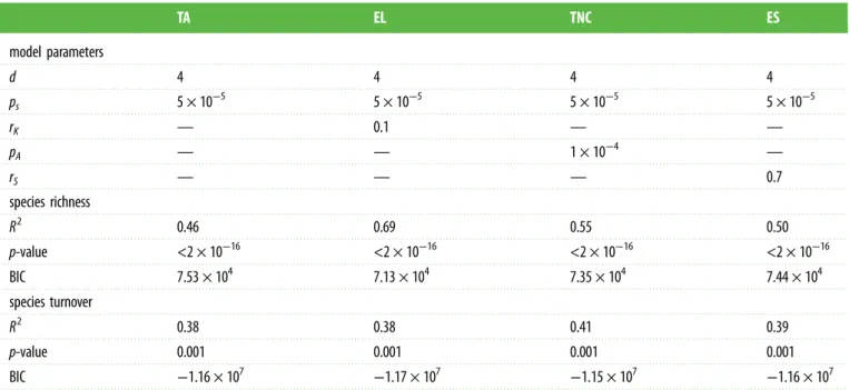
Table 1. Model parameters of the best simulations run under the under the TA, EL, TNC and ES models. (For each best simulation, the goodness-of-

fit measures

(BIC and R

) that were used to compare simulated and observed data for species richness and

β-diversity caused by species turnover are also shown (see methods

and the electronic supplementary material for more details).)

TA

EL

TNC

ES

model parameters

d

4

4

4

4

p

5 × 10

5 × 10

5 × 10

5 × 10

r

—

0.1

—

—

p

—

—

1 × 10

—

r

—

—

—

0.7

species richness

R

0.46

0.69

0.55

0.50

p-value

<2 × 10

<2 × 10

<2 × 10

<2 × 10

BIC

7.53 × 10

7.13 × 10

7.35 × 10

7.44 × 10

species turnover

R

0.38

0.38

0.41

0.39

p-value

0.001

0.001

0.001

0.001

BIC

−1.16 × 10

−1.17 × 10

−1.15 × 10

−1.16 × 10

http://doc.rero.ch

(ii) Time-area

The TA model predicted the formation of the LDG during the middle Eocene (figure 3a; electronic supplementary material, figure S3a). Compared to the observed LDG, the TA model over-estimated species richness at subtropical and temperate latitudes (greater than 26° N), with latitudinal breaks in species

richness for the Indo-Pacific region at−22° N and 46° N and for

the Atlantic region at 18° N (figure 3a; electronic supplemen-tary material, figure S3a and table S1). This model did not generate any latitudinal breaks in species turnover in the past (electronic supplementary material, figure S9a).

(iii) Tropical niche conservatism

The TNC model predicted a steeper and narrower modern LDG (figure 3b; electronic supplementary material, figure S3b) than the TA model, with breaks in species richness at −18° N and 23° N for the Indo-Pacific region and breaks

at −2° N and 30° N for the Atlantic region (electronic

supplementary material, table S1). We also did not observe any latitudinal breaks in species turnover (electronic sup-plementary material, figure S9b). The TNC model predicted a steep decline in species richness towards the tropics begin-ning at the end of the Miocene owing to the contraction of the tropics (figure 3b; electronic supplementary material, figures S13 and S14). Notably, this model generated high poleward dispersal rates during the late Cretaceous and early Palaeo-gene, despite the strong dispersal constraint that we imposed.

(iv) Ecological limits

The EL model predicted a strong LDG with breaks in species

richness at−19° N and 23° N and −21° N and 29° N for the

Indo-Pacific and Atlantic regions, respectively (figure 3c; elec-tronic supplementary material, figure S3c). Similar to the TNC model, the EL model revealed a steep decline in species richness towards the poles in relation to the contraction of the tropics during the Pliocene and Quaternary periods.

0.4

speciation rate

speciation extinction dispersion

extinction rate dispersion rate

0.12 0 0.02 0.04 0.06 0.08 0.10 0.3 0.2 0.1

Cretaceous Palaeogene Neogene Cretaceous Palaeogene Neogene Cretaceous Palaeogene Neogene

Cretaceous Palaeogene Neogene Cretaceous Palaeogene Neogene Cretaceous Palaeogene Neogene

Cretaceous Palaeogene Neogene Cretaceous Palaeogene Neogene Cretaceous Palaeogene Neogene

Cretaceous Palaeogene Neogene Cretaceous Palaeogene Neogene Cretaceous Palaeogene Neogene

0 0.4 0.3 0.2 0.1 0 0.4

speciation rate extinction rate dispersion rate

0.12 0 0.02 0.04 0.06 0.08 0.10 0.3 0.2 0.1 0 0.4 0.3 0.2 0.1 0 0.4

speciation rate extinction rate dispersion rate

0.12 0 0.02 0.04 0.06 0.08 0.10 0.3 0.2 0.1 0 0.4 0.3 0.2 0.1 0 0.4

speciation rate extinction rate dispersion rate

0.12 0 0.02 0.04 0.06 0.08 0.10 0.3 0.2 0.1 0 0.4 0.3 0.2 0.1 0 (a) (b) (c) (d)

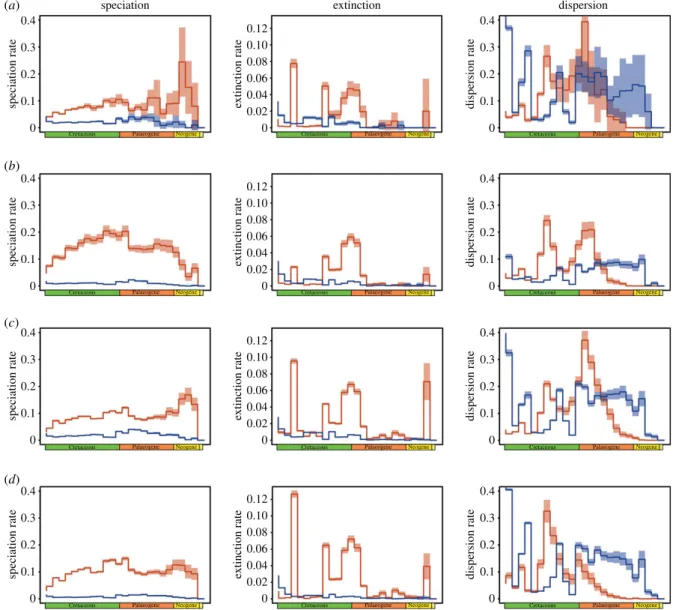
Figure 2. Diversification rates through time from each model under sympatric speciation. We calculated the speciation, extinction and dispersal rates of tropical and

temperate lineages in each simulation for time periods of 5 Myr. The rates are calculated as the number of events (inside and outside the tropics) divided by the

number of lineages (tropical and temperate lineages, respectively) divided by the length of the time period (here, 5 Myr). The rates are thus expressed as events per

species per Myr. Note that widespread lineages are considered both tropical and temperate. For each mechanism, we calculated the rates for the 10 simulations run

with the set of parameters that rendered the best simulations. (a) The TA model, (b) the TNC model, (c) the EL model and (d ) the ES model. In the first two

columns, orange represents the tropical lineages and blue the temperate lineages. In the third column, orange represents the dispersal towards the poles and blue

the dispersal towards the tropics. (Online version in colour.)

Furthermore, the EL model predicted strong latitudinal breaks in species turnover at high latitudes (electronic sup-plementary material, figure S9c). The EL model generated globally lower speciation rates and higher extinction rates of tropical lineages than the TA and TNC models (figure 3).

(v) Evolutionary speed

Similar to the TA model, the ES model generated a slight

LDG with breaks in species richness at −23° N and 46° N

for the Indo-Pacific region and breaks at 2.9° N and 40° N for the Atlantic region (figure 3d; electronic supplementary material, figure S3d). We did not observe a significant latitu-dinal break in species turnover (electronic supplementary material, figure S9d). The ES model generated globally

lower speciation rates and higher extinction rates of tropical lineages than the TA and TNC models (figure 3).

4. Discussion

The uneven distribution of biodiversity on Earth ultimately results from the heterogeneous outcome of speciation, extinc-tion and dispersal [40,41]. Various historical and ecological factors have been proposed to explain biodiversity gradients [3–5]. However, we still lack integrated models that can be used to evaluate the effect of these different factors and their interactions [42]. In this study, we use a mechanistic modelling approach to evaluate how historical and ecological factors may influence reef fish diversity in space and time according to alternative hypotheses. Our results reveal that palaeohabitat dynamics determined the LDG in reef fishes during deep geo-logical time but that only ecogeo-logical constraints related to the contraction of the tropical habitat during the Neogene (−23 to 2.5 Myr) explain the current shape of the LDG.

Habitat dynamics are expected to be major determinants of biodiversity gradients [5,9]. For example, several studies have shown that species richness and composition are closely linked to habitat changes caused by past tectonic events [9,29,43–45]. However, owing to the lack of palaeoenvironmen-tal and palaeontological data, little empirical evidence supports the influence of past habitat dynamics on the LDG [5,18]. In the simulations run under the TA hypothesis, large and stable areas of tropical habitat (electronic supplementary material, figure S13) maintained high diversification rates (electronic

supplementary material, figure S15), which gradually

increased species richness in the tropics (figure 3a). These simu-lations also revealed a slowdown of tropical lineages’ speciation rates during the Neogene (figure 2a), with relatively similar speciation rates between tropical and temperate lineages at the end of the Neogene, which could be related to the shrinkage of tropical reef habitats during this period (elec-tronic supplementary material, figures S13 and S14). This result is particularly consistent with a recent phylogenetic-based study [21] that showed relatively little variation in recent spe-ciation rates in marine fishes for the latitudinal range that we

considered here (i.e. between−60° and 60° N, see the electronic

supplementary material, figure S16 for acanthomorph reef fishes). Overall, these findings provide support for the hypoth-esis that the LDG is the result of the deep-time history of clades in relation to the dynamics of tropical habitats [46–49], hence explaining the temporal variability in this pattern [50].

Although palaeohabitat dynamics alone can generate an LDG in reef fishes, the TA model failed to predict all the fea-tures of the modern LDG, such as the position of latitudinal breakpoints in species richness. Indeed, the TA model was found to over-estimate species richness at subtropical and temperate latitudes, especially in the Northern Hemisphere (figure 2a). The addition of mechanisms considering the response of species to climatic conditions, as proposed by the EL and TNC hypotheses, markedly improved the predic-tion of the latitudinal variapredic-tion in both species richness and species turnover. This result suggests that the steepness of the LDG and observed latitudinal breaks in species turnover are generated by ecological constraints acting at the limits between tropical and temperate environments. This mechan-ism is not unexpected, given that contemporary patterns of species richness and species turnover are strongly associated

60 obs. obs. obs. obs. latitude –60 –40 –20 0 20 40 60 latitude –60 –40 –20 0 20 40 60 latitude –60 –40 –20 0 20 40 60 latitude –60 0 564

Palaeocene Eocene Oligocene Miocene Pli. Ple. H. Palaeocene Eocene Oligocene Miocene Pli. Ple. H. Palaeocene Eocene Oligocene Miocene Pli. Ple. H. Palaeocene Eocene Oligocene Miocene Pli. Ple. H.

1128 1692 latitudinal richness 2256 2820 –40 –20 0 20 40 (a) (b) (c) (d)

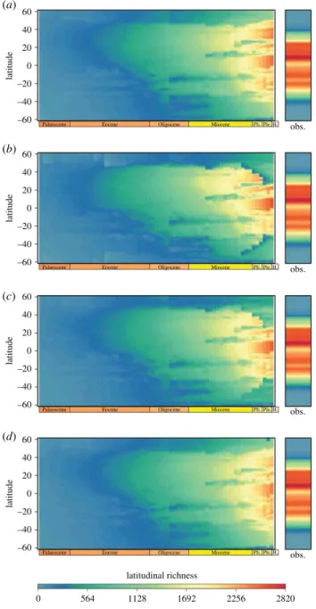
Figure 3. Evolution of the LDG in reef fishes according to simulations run under

(a) the TA model, (b) the TNC model, (c) the EL model and (d) the ES model. We

present the latitudinal variation in reef fish species richness during geological periods

from the Palaeocene to the Holocene. For each mechanism, we calculated the

species richness of the best simulation across latitudes at each time step. These

simulated patterns can be compared to the observed latitudinal variation in species

richness located on the right of each plot (obs.). Pli, Pliocene; Ple, Pleistocene; H,

Holocene.

with climatic conditions [45,51]. The fossil record also shows that past climatic changes left a strong imprint on the LDG [50,52,53], while comparative studies have demonstrated the importance of climatic variations in diversification dynamics [25,54]. In our simulations, palaeohabitat dynamics controlled global differences in species richness and diversification rates between tropical and extratropical areas, while climate-based processes controlled the steepness of the species richness gradi-ent and the position of latitudinal breaks in species turnover. Consequently, these mechanisms are expected to act in concert to shape the LDG at different spatial and temporal scales.

However, differentiating the predictions of alternative climate-based mechanisms (i.e. mechanisms considering a response to climatic conditions) using our model remains challenging. First, the ES model generates predictions similar to those of the TA model, which makes these processes difficult to differentiate in comparative studies. This suggests that the full complexity of the LDG cannot be predicted by simple differences in speciation rates between tropical and temperate lineages. Second, the EL and TNC models yield more realistic predictions of the latitudinal variation in

species richness and β-diversity (electronic supplementary

material, figure S6). In the literature, one can find evidence supporting both hypotheses. On the one hand, studies focusing on the influence of palaeotemperature variations on extinction rates of tropical lineages suggest that niche conservatism limits species adaptation to a changing envi-ronment [54]. On the other hand, the results from studies focusing on density dependence support a difference in car-rying capacity between temperate and tropical regions [55]. When evaluated jointly, both mechanisms seem to influence different macroevolutionary processes [25], suggesting that their relative influences could work closely together [56]. In our simulations, we observed small differences in the predic-tions of these hypotheses. Overall, the EL model rendered better predictions for the variables we chose. Notably, it gen-erated more obvious latitudinal breaks in species turnover. In this case, new species that appeared inside a biome (tropical or temperate) outcompeted those that colonized the biome, limiting exchanges between biomes and increasing species replacement at the boundaries between tropical and temper-ate habitats. Furthermore, according to the EL model, the saturation of temperate habitats prevented the speciation rates of temperate lineages from increasing at the end of the Neogene, despite the expansion of temperate habitats (elec-tronic supplementary material, figures S13 and S14). In both EL and TNC simulations, the position of the boundary between tropical and temperate environments is key. Thus, our predictions using those models should be interpreted carefully as they are dependent on the reef-forming corals fossil record that we used as a proxy for tropical climate. Hence, the tropical limit is an approximation that might suffer from dating, palaeo-localization inaccuracy or data gap, especially further back in time ([57], electronic supplementary material, Discussion).

This study demonstrates the importance of using multiple biodiversity metrics to evaluate alternative hypotheses in the fields of ecology, evolution and biogeography rather than focusing on a single diversity metric [25]. Our results showed that considering not only species richness but also β-diversity allows better comprehension of the mechanisms shaping the LDG. Our findings also illustrate the importance of the temporal scale used when evaluating how alternative

hypotheses may explain the modern LDG. In all our

simu-lations, the tropics were considered either ‘a cradle’ or ‘a

museum’ [58], depending on the time scale. Tropical habitats can be considered cradles on a very deep time scale because most lineages originated in the tropics owing to a much warmer climate and extensive tropical and subtropical habitat in the Mesozoic (figures 2 and 3). Tropical habitats can also be considered museums on a shorter time scale because they allowed the survival of tropical lineages during the expansion of temperate habitats starting in the middle of the Neogene.

The OTT ([10]) model posits that the tropics support more species because lineages there have higher speciation rates, lower extinction rates and higher net emigration over immigration than do lineages in extratropical regions. Our simulations based solely on the influence of habitat dynamics

tend to support the predictions of the‘OTT’ model from the

mid-Cretaceous to the mid-Palaeogene but tend to reject it for other time periods, which stresses the temporal charac-teristic of this model [59]. Furthermore, even with a strong influence of TNC, our simulations under the sympatric mode of speciation revealed a higher net rate of emigration over immigration in tropical lineages than in temperate lineages in those time periods. Given this perspective, the results from macroevolutionary models should be interpreted carefully as an estimate of higher rates of dispersal towards temperate habitats for lineages with tropical origins does not always constitute evidence against TNC [20,23]. In that sense, our results are concordant with the findings of Siqueira et al. [23], but allowed a deeper understanding of the poten-tial causes of differences in diversification rates and temporal shifts in dispersal rates in reef fishes.

5. Conclusion and perspectives

In this study, we showed that the additional consideration of climate-based processes in the habitat-driven SPLIT model [9,28] significantly improved predictions of the modern LDG. Using a process-based modelling approach, we revealed how large-scale macroevolutionary dynamics and in situ environ-mental processes can interact in space and time to generate observed patterns of biodiversity. The simple formalism of the model presented in this study allows a broad range of modi-fications and improvements [28], facilitating the integration of a more complex process. We suggest that incorporating competition and trait evolution under selective pressures in a moving landscape could allow prediction of greater

differ-ences in β-diversity and evolutionary rates with alternative

mechanisms. This kind of model would consider process-based mechanisms to establish a link between micro- and macroevolutionary scales [60].

Data accessibility.The data supporting the results will be archived in the Dryad Digital Repository: https://doi.org/10.5061/dryad.0r852nm [61]. The SPLIT model with associated palaeoenvironmental data can be found at https://github.com/theogab/SPLIT.

Authors’ contributions. T.G., L.P. and F.L. conceived and designed the study. C.A. provided the reef fish occurrence database. T.G. per-formed the analyses with the help of C.A. and P.D. All the authors discussed the results. T.G. and F.L. led the writing, and all authors contributed substantially to finalizing this manuscript.

Competing interests.We declare we have no competing interests.

Funding.This work was financed by the ANR-FNS REEFISH project no. 310030E-164294 and supported by a Doctoral School GAIA.

References

1. Hillebrand H. 2004 On the generality of the

latitudinal diversity gradient. Am. Nat. 163,

192–211.

(doi:10.1146/annurev-ecolsys-112414-054102)

2. Kinlock NL et al. 2018 Explaining global variation in

the latitudinal diversity gradient: meta-analysis confirms known patterns and uncovers new ones.

Glob. Ecol. Biogeogr. 27, 125–141. (doi:10.1111/

geb.12665)

3. Willig MR, Kaufman DM, Stevens RD. 2003

Latitudinal gradients of biodiversity: patterns, scale, and synthesis. Annu. Rev. Ecol. Evol. Syst. 34,

273–309. (doi:10.1146/annurev.ecolsys.34.012103.

144032)

4. Mittelbach GG et al. 2007 Evolution and the

latitudinal diversity gradient: speciation, extinction

and biogeography. Ecol. Lett. 10, 315–331. (doi:10.

1111/j.1461-0248.2007.01020.x)

5. Fine PVA. 2015 Ecological and evolutionary drivers

of geographic variation in species diversity. Annu.

Rev. Ecol. Evol. Syst. 46, 369–392. (doi:10.1146/

annurev-ecolsys-112414-054102)

6. Jetz W, Fine PVA. 2012 Global gradients in

vertebrate diversity predicted by historical area-productivity dynamics and contemporary environment. PLoS Biol. 10, e1001292. (doi:10. 1371/journal.pbio.1001292)

7. Rosenzweig ML. 1995 Species diversity in space and

time, p. 436. Cambridge, UK: Cambridge University Press.

8. Leprieur F, Descombes P, Gaboriau T, Cowman PF,

Parravicini V. 2016 Plate tectonics drive tropical reef biodiversity dynamics. Nat. Commun. 7, 11461. (doi:10.1038/ncomms11461)

9. Descombes P, Gaboriau T, Albouy C, Heine C,

Leprieur F, Pellissier L. 2017 Linking species diversification to palaeo-environmental changes: a process-based modelling approach. Glob. Ecol.

Biogeogr. 27, 233–244. (doi:10.1111/geb.12683)

10. Wiens JJ et al. 2010 Niche conservatism as an emerging principle in ecology and conservation

biology. Ecol. Lett. 13, 1310–1324. (doi:10.1111/j.

1461-0248.2010.01515.x)

11. Hutchinson GE. 1959 Homage to Santa Rosalia or why are there so many kinds of animals? Am. Nat.

93, 145–159. (doi:10.1086/282070)

12. MacArthur R. 1965 Patterns of species diversity. Biol. Rev. Camb. Philos. Soc. 40, 510. (doi:10.1111/j. 1469-185X.1965.tb00815.x)

13. Rohde K. 1992 Latitudinal gradients in species diversity: the search for the primary cause. Oikos 65, 514. (doi:10.2307/3545569)

14. Allen AP, Gillooly JF, Savage VM, Brown JH. 2006 Kinetic effects of temperature on rates of genetic divergence and speciation. Proc. Natl Acad. Sci. USA

103, 9130–9135. (doi:10.1073/pnas.0603587103)

15. Allen AP, Brown JH, Gillooly JF. 2002 Global biodiversity, biochemical kinetics, and the

energetic-equivalence rule. Science 297, 1545–1548. (doi:10.

1126/science.1072380)

16. Brown JH. 2014 Why are there so many species

in the tropics? J. Biogeogr. 41, 8–22. (doi:10.1111/

jbi.12228)

17. Sandel B, Dangremond EM. 2012 Climate change and the invasion of California by grasses. Glob.

Chang. Biol. 18, 277–289.

(doi:10.1111/j.1365-2486.2011.02480.x)

18. Belmaker J, Jetz W. 2015 Relative roles of ecological and energetic constraints, diversification rates and region history on global species richness gradients.

Ecol. Lett. 18, 563–571. (doi:10.1111/ele.12438)

19. Gavin MC et al. 2017 Process-based modelling shows how climate and demography shape language diversity. Glob. Ecol. Biogeogr. 26,

584–591. (doi:10.1111/geb.12563)

20. Rolland J, Condamine FL, Jiguet F, Morlon H. 2014 Faster speciation and reduced extinction in the tropics contribute to the mammalian latitudinal diversity gradient. PLoS Biol. 12, e1001775. (doi:10. 1371/journal.pbio.1001775)

21. Rabosky DL et al. 2018 An inverse latitudinal gradient in speciation rate for marine fishes. Nature

559, 392–395. (doi:10.1038/s41586-018-0273-1)

22. Goldberg EE, Lancaster LT, Ree RH. 2011 Phylogenetic inference of reciprocal effects between geographic range evolution and

diversification. Syst. Biol. 60, 451–465. (doi:10.

1093/sysbio/syr046)

23. Siqueira AC, Oliveira-Santos LGR, Cowman PF, Floeter SR, Algar A. 2016 Evolutionary processes underlying latitudinal differences in reef fish

biodiversity. Glob. Ecol. Biogeogr. 25, 1466–1476.

(doi:10.1111/geb.12506)

24. Buckley LB et al. 2010 Phylogeny, niche conservatism and the latitudinal diversity gradient

in mammals. Proc. R. Soc. B 277, 2131–2138.

(doi:10.1098/rspb.2010.0179)

25. Lehtonen S et al. 2017 Environmentally driven extinction and opportunistic origination explain fern diversification patterns. Sci. Rep. 7, 4831. (doi:10. 1038/s41598-017-05263-7)

26. Pellissier L, Heine C, Rosauer DF, Albouy C. 2018 Are global hotspots of endemic richness shaped by

plate tectonics? Biol. J. Linn. Soc. 123, 247–261.

(doi:10.1111/brv.12366)

27. Albert JS, Schoolmaster DR, Tagliacollo V, Duke-Sylvester SM. 2017 Barrier displacement on a neutral landscape: toward a theory of continental

biogeography. Syst. Biol. 66, 167–182. (doi:10.

1093/sysbio/syw080)

28. Janzen DH. 1967 Why mountain passes are higher

in the tropics? Am. Nat. 101, 233–249. (doi:10.

1086/282487)

29. Jordan SMR, Barraclough TG, Rosindell J. 2016 Quantifying the effects of the break up of Pangaea on global terrestrial diversification with neutral theory. Phil. Trans. R. Soc. B 371, 20150221. (doi:10.1098/rstb.2015.0221)

30. Rangel TF et al. 2018 Modeling the ecology and evolution of biodiversity: biogeographical cradles,

museums, and graves. Science 361, eaar5452. (doi:10.1126/science.aar5452)

31. Bellwood DR, Hughes TP, Connolly SR, Tanner J. 2005 Environmental and geometric constraints on Indo-Pacific coral reef biodiversity. Ecol. Lett. 8,

643–651. (doi:10.1111/j.1461-0248.2005.00763.x)

32. Price SA, Claverie T, Near TJ, Wainwright PC. 2015 Phylogenetic insights into the history and diversification of fishes on reefs. Coral Reefs 34,

997–1009. (doi:10.1007/s00338-015-1326-7)

33. Müller RD, Sdrolias M, Gaina C, Steinberger B, Heine C. 2008 Long-term sea-level fluctuations driven by

ocean basin dynamics. Science 319, 1357–1362.

(doi:10.1126/science.1151540)

34. Poyato-Ariza FJ. 1996 A revision of Rubiesichthys gregalis Wenz 1984 (Ostariophysi,

Gonorynchiformes), from the Early Cretaceous of

Spain. Syst. Paleoecol. 1984, 329–348.

35. Baselga A. 2010 Partitioning the turnover and nestedness components of beta diversity. Glob. Ecol.

Biogeogr. 19, 134–143. (doi:10.1111/j.1466-8238.

2009.00490.x)

36. Baselga A, Orme CDL. 2012 Betapart: an R package for the study of beta diversity. Methods Ecol. Evol. 3,

808–812. (doi:10.1111/j.2041-210X.2012.00224.x)

37. Lichstein JW. 2006 Multiple regression on distance matrices: a multivariate spatial analysis tool. Plant

Ecol. 188, 117–131. (doi:10.1007/s11258-006-9126-3)

38. Muggeo VM. 2008 Segmented: an R package to fit regression models with broken-line relationships.

R News 20–25, 1–73.

39. R Core Team. 2019 R: a language and environment for statistical computing. Vienna, Austria: R Foundation for Statistical Computing. See https:// www.r-project.org.

40. Ricklefs RE. 1987 Community diversity: relative roles of local and regional processes. Science 235,

167–171. (doi:10.1126/science.235.4785.167)

41. Schluter D, Pennell MW. 2017 Speciation gradients and the distribution of biodiversity. Nature 546,

48–55. (doi:10.1038/nature22897)

42. Gotelli NJ et al. 2009 Patterns and causes of species richness: a general simulation model for

macroecology. Ecol. Lett. 12, 873–886. (doi:10.

1111/j.1461-0248.2009.01353.x)

43. Renema W et al. 2008 Hopping hotspots: global

shifts in marine biodiversity. Science 321, 654–657.

(doi:10.1126/science.1155674)

44. Descombes P, Leprieur F, Albouy C, Heine C, Pellissier L. 2017 Spatial imprints of plate tectonics on extant richness of terrestrial

vertebrates. J. Biogeogr. 44, 1185–1197. (doi:10.

1111/jbi.12959)

45. Mazel F, Wüest RO, Lessard J-P, Renaud J, Ficetola GF, Lavergne S, Thuiller W. 2017 Global patterns of β-diversity along the phylogenetic time-scale: the role of climate and plate tectonics. Glob. Ecol.

Biogeogr. 26, 1211–1221. (doi:10.1111/geb.12632)

46. Fine PVA, Ree RH. 2006 Evidence for a time-integrated species-area effect on the latitudinal

gradient in tree diversity. Am. Nat. 168, 796–804. (doi:10.1086/508635)

47. Jablonski D, Kaustuv R, Valentine JW. 2006 Out of the tropics: evolutionary diversity gradient. Science 314,

102–106. (doi:10.1126/science.1130880)

48. Cowman PF, Parravicini V, Kulbicki M, Floeter SR. 2017 The biogeography of tropical reef fishes: endemism and provinciality through time. Biol. Rev.

92, 2112–2130. (doi:10.1111/brv.12323)

49. Miller EC, Hayashi KT, Song D, Wiens JJ. 2018

Explaining the ocean’s richest biodiversity hotspot

and global patterns of fish diversity. Proc. R. Soc. B 285, 20181314. (doi:10.1098/rspb.2018.1314) 50. Mannion PD, Upchurch P, Benson RBJ, Goswami A.

2014 The latitudinal biodiversity gradient through

deep time. Trends Ecol. Evol. 29, 42–50. (doi:10.

1016/j.tree.2013.09.012)

51. Tittensor DP, Mora C, Jetz W, Lotze HK, Ricard D, Berghe EV, Worm B. 2010 Global patterns and predictors of marine biodiversity across taxa. Nature

466, 1098–1101. (doi:10.1038/nature09329)

52. Crame JA. 2001 Taxonomic diversity gradients

through geological time. Divers. Distrib. 7, 175–189.

(doi:10.1046/j.1472-4642.2001.00106.x) 53. Fenton IS, Pearson PN, Jones TD, Farnsworth A,

Lunt DJ, Markwick P, Purvis A. 2016 The impact of Cenozoic cooling on assemblage diversity in planktonic foraminifera. Phil. Trans. R. Soc. B 371, 20150224. (doi:10.1098/rstb. 2015.0224)

54. Kergoat GJ et al. 2014 Cretaceous environmental changes led to high extinction rates in a hyperdiverse beetle family. BMC Evol. Biol. 14, 220. (doi:10.1186/s12862-014-0220-1)

55. Machac A, Graham CH. 2017 Regional diversity and

diversification in mammals. Am. Nat. 189, E1–E13.

(doi:10.1086/689398)

56. Tomašových A, Jablonski D. 2017 Decoupling of

latitudinal gradients in species and genus geographic range size: a signature of clade range

expansion. Glob. Ecol. Biogeogr. 26, 288–303.

(doi:10.1111/geb.12533)

57. Edinger EN, Burr GS, Pandolfi JM, Ortiz JC. 2007 Age accuracy and resolution of Quaternary corals used as proxies for sea level. Earth Planet. Sci. Lett. 253,

37–49. (doi:10.1016/j.epsl.2006.10.014)

58. Stebbins GL. 1974 Flowering plants: evolution above the species level, 480 p. Cambridge, MA: Belknap Press. 59. Huang S, Roy K, Jablonski D. 2014 Do past

climate states influence diversity dynamics and the present-day latitudinal diversity gradient? Glob.

Ecol. Biogeogr. 23, 530–540. (doi:10.1111/geb.12153)

60. Pontarp M et al. 2018 The latitudinal diversity gradient: novel understanding through mechanistic eco-evolutionary models.

Trends Ecol. Evol. 24, P211–223. (doi:10.1016/j.tree.

2018.11.009)

61. Gaboriau T, Albouy C, Descombes P, Mouillot D, Pellissier L, Leprieur F. 2019 Data from: Ecological constraints coupled with deep-time habitat dynamics predict the latitudinal diversity gradient in reef fishes. Dryad Digital Repository. (http://doi.org/ 10.5061/dryad.0r852nm)