HAL Id: hal-02267200
https://hal.archives-ouvertes.fr/hal-02267200
Submitted on 19 Aug 2019
HAL is a multi-disciplinary open access archive for the deposit and dissemination of sci-entific research documents, whether they are pub-lished or not. The documents may come from teaching and research institutions in France or abroad, or from public or private research centers.
L’archive ouverte pluridisciplinaire HAL, est destinée au dépôt et à la diffusion de documents scientifiques de niveau recherche, publiés ou non, émanant des établissements d’enseignement et de recherche français ou étrangers, des laboratoires publics ou privés.
Prediction of CO 2 absorption by physical solvents using
a chemoinformatics-based machine learning model
Hao Li, Dan Yan, Zhien Zhang, Eric Lichtfouse
To cite this version:
Hao Li, Dan Yan, Zhien Zhang, Eric Lichtfouse. Prediction of CO 2 absorption by physical solvents using a chemoinformatics-based machine learning model. Environmental Chemistry Letters, Springer Verlag, 2019, 17 (3), pp.1397 - 1404. �10.1007/s10311-019-00874-0�. �hal-02267200�
https://doi.org/10.1007/s10311-019-00874-0 ORIGINAL PAPER
Prediction of CO
2absorption by physical solvents using
a chemoinformatics‑based machine learning model
Hao Li1 · Dan Yan2 · Zhien Zhang3 · Eric Lichtfouse4
Received: 22 December 2018 / Accepted: 2 March 2019 / Published online: 18 March 2019 © Springer Nature Switzerland AG 2019
Abstract
The rising atmospheric CO2 level is partly responsible for global warming. Despite numerous warnings from scientists
dur-ing the past years, nations are reactdur-ing too slowly, and thus, we will probably reach a situation needdur-ing rapid and effective techniques to reduce atmospheric CO2. Therefore, advanced engineering methods are particularly important to decrease the greenhouse effect, for instance, by capturing CO2 using solvents. Experimental testing of many solvents under different
con-ditions is necessary but time-consuming. Alternatively, modeling CO2 capture by solvents using a nonlinear fitting machine
learning is a rapid way to select potential solvents, prior to experimentation. Previous predictive machine learning models were mainly designed for blended solutions in water using the solution concentration as the main input of the model, which was not able to predict CO2 solubility in different types of physical solvents. To address this issue, here, we developed a new
descriptor-based chemoinformatics model for predicting CO2 solubility in physical solvents in the form of mole fraction. The
input factors include organic structural and bond information, thermodynamic properties, and experimental conditions. We studied the solvents from 823 data, including methanol (165 data), ethanol (138), n-propanol (98), n-butanol (64), n-pentanol (59), ethylene glycol (52), propylene glycol (54), acetone (51), 2-butanone (49), ethylene glycol monomethyl ether (46 data), and ethylene glycol monoethyl ether (47), using artificial neural networks as the machine learning model. Results show that our descriptor-based model predicts the CO2 absorption in physical solvents with generally higher accuracy and low root-mean-squared errors. Our findings show that using a set of simple but effective chemoinformatics-based descriptors, intrinsic relationships between the general properties of physical solvents and their CO2 solubility can be precisely fitted
with machine learning.
Keywords Chemoinformatics · Greenhouse gas · CO2 · Absorption · Solubility · Physical solvent · Chemical descriptors · Prediction · Machine learning · Artificial neural network (ANN)
Introduction
Carbon dioxide (CO2) is a major greenhouse gas inducing
worldwide global warming (Krupa and Kickert 1993). The global CO2 level increased to more than 408 parts per mil-lion (ppm) in 2018 compared to about 300 ppm in 1950s (Zhang et al. 2018c, https ://www.co2.earth ). Combustion of chemicals in industry can also lead to significant increase in CO2 levels within a short period (Liu et al. 2014, 2018a, b). Therefore, engineering methods are currently developed to decrease CO2 levels rapidly. For instance, CO2
electrochemi-cal reduction and collection reduces CO2 emission from the usage of fuel cells (Adzic et al. 2007; Li and Henkelman
2017; Li et al. 2018a, b, c). Electrochemical reduction also provides carbon sources for higher value product formation via electrochemistry (Aeshala et al. 2013; Padilla et al. 2017; Electronic supplementary material The online version of this
article (https ://doi.org/10.1007/s1031 1-019-00874 -0) contains supplementary material, which is available to authorized users. * Zhien Zhang
[email protected]; [email protected]
1 Department of Chemistry and the Institute
for Computational and Engineering Sciences, The University of Texas at Austin, 105 E. 24th Street, Stop A5300, Austin, TX 78712, USA
2 Shenzhen Environmental Science and Technology
Engineering Laboratory, Tsinghua-Berkeley Shenzhen Institute, Tsinghua University, Shenzhen 518055, China
3 William G. Lowrie Department of Chemical
and Biomolecular Engineering, The Ohio State University, Columbus, OH 43210, USA
4 CEREGE, Aix-Marseille Univ, Coll de France, CNRS,
INRA, IRD, Aix-en-Provence, France
1398 Environmental Chemistry Letters (2019) 17:1397–1404
1 3
Singh et al. 2017). However, the main drawback of electro-reduction is that it cannot directly use the atmospheric CO2, which could lead to additional cost for the CO2 capture.
On the other hand, liquid-based chemical absorption is a common method for CO2 capture (Aaron and Tsouris 2005;
Yu et al. 2012; Li et al. 2013; Zhang et al. 2018a; Koyt-soumpa et al. 2018). There are some widely reported absor-bents, including physical solvents (Gui et al. 2011), alkali (Tontiwachwuthikul et al. 1992), alkanolamine (Paul et al.
2008), ionic liquids (Dai et al. 2015), and amino acid salts solutions (Wei et al. 2014). Although there are many advanced methods for CO2 capturing, the most commonly
used and economical solvent-based process in industry is still using physical solvents (Gui et al. 2011). Physical sol-vents are non-corrosive compared with chemical solsol-vents, requiring only carbon steel construction. Physical solvents such as methanol involve physical affinities such as polarity to dissolve a compound, whereas chemical solvents such as ethanolamines and potassium carbonate rely on chemical reactions. The aim of this paper is to accurately predict the CO2 solubility in physical solvents at relatively high pressure
because higher pressure favors CO2 recovery.
Testing solvents for CO2 capture requires numerous
experiments to assess optimal conditions, for instance, vapor–liquid equilibrium (VLE) experiments with varying temperatures and CO2 partial pressures, leading to high labor works and economic costs (Zhang et al. 2018b). To address this issue, machine learning modeling has been proven as a powerful tool to directly predict the CO2 solubility in
solu-tion, with the simple input data of solution concentrations, temperature, and partial CO2 pressures (Zhang et al. 2018b).
Recently, it was found that a generalized input representa-tion that includes different components and composirepresenta-tions of blended solutions (solutions with mixture of at least two components) can precisely predict the CO2 solubility
in seven types of blended solutions (Li and Zhang 2018). Also, due to the nonlinear intrinsic trends of CO2 solubility,
mining the intrinsic trends of CO2 solubility with varying experimental conditions is particularly important. Previ-ous studies have found that, compared with other theoreti-cal methods, e.g., equation of states (EOS) (Duan and Sun
2003), molecular dynamics (MD) (Murad and Gupta 2000), and polynomial fittings, a knowledge-based machine learn-ing can help to mine the intrinsic relationships of CO2
solu-bility with high accuracy and much lower computational costs. This indicates that a machine learning model can help to predict the performance of a CO2 absorbent and optimize
its experimental conditions, in a very cost-effective way. Nonetheless, contrary to blended solutions, it is rather difficult to predict the CO2 solubility in physical solvents (pure organic solvent without solute) because such a pre-diction requires precise descriptors that could identify and differentiate different molecular structures. Currently, there
are some state-of-the-art descriptors for atomistic simula-tions, also named ‘fingerprints’ that could capture the atomic interactions in an atomistic system (Behler and Parrinello
2007; Li et al. 2017b). However, it sometimes requires a large number of input data with varying hyper-parameters, which limits the training efficiency of the model for non-atomistic simulations.
To predict CO2 solubility in physical solvents, in this
let-ter, we address this issue by proposing a set of novel chem-oinformatics-based descriptors for organic molecules, with the input data of structural and bond information, molecu-lar thermodynamic properties, and experimental conditions. Using 823 data of 11 physical solvents extracted from exper-imental literature, we found that such a novel representa-tion can help to precisely capture the intrinsic relarepresenta-tionships between the physical solvent and CO2 solubility. With
rigor-ous model evaluations, we found that such a model is gen-eral enough to predict the CO2 solubility in organic solvents with high accuracy, which could help to dramatically reduce experimental budgets of looking for promising solvents and optimal conditions for CO2 capture.
Experimental
DescriptorsTo predict the CO2 solubility in various physical solvents,
the input data of the models should include the descriptors that fully describe the structural and bond information, rele-vant thermodynamic properties, and experimental operating conditions. To describe the structural and bond information, in this study, we included the number of each element (C, H, and O), number of bonds (C–C, C–H, O–H, C–O, and C=O), molecular weight, numbers of hydrogen donors and acceptors, number of rotatable bond, and molecular com-plexity (the quantitative structural comcom-plexity of a molecule (Böttcher 2016)), as the inputs of the model. To provide more information that is potentially relevant to the solubility, several thermodynamic properties including density, vapor density, vapor pressure, dipole moment, and boiling point were also used as input variables. Note that all these data can be easily found from previous experimental measure-ments in online database. In our study, all these properties were extracted from PubChem (Wang et al. 2009). Our pre-liminary algorithmic testings show that though the modeling accuracies majorly depend on the input data of structural and bond information, the use of these thermodynamic proper-ties as the input data could further lower down the prediction errors. To test the experimental conditions, temperature and the operating CO2 partial pressure are also used as the input
variables (Bezanehtak et al. 2002; Tsivintzelis et al. 2004; Secuianu et al. 2008, 2009; Yim et al. 2010; Gui et al. 2011).
Modeling
Machine learning and other algorithmic methods are pow-erful techniques that can help to address both scientific and engineering issues (Park and Jun 2013, 2015). Here, we used artificial neural networks (ANNs) as the machine learning algorithm for data training (Zhang et al. 1998; Li
et al. 2017a). Specifically, general regression neural network (GRNN) (Specht 1991) and multilayer feed-forward neural network (Hornik et al. 1989; Svozil et al. 1997) with a back-propagation optimization, namely back-back-propagation neural network (BPNN) (Nawi et al. 2013), were used as the algo-rithms. In order to determine the best BPNN, different net-work architectures of BPNN were modeled. In this article, BPNNs with different numbers of hidden layers and neurons are denoted as X–N–Y and X–N–N–Y, where X is the number
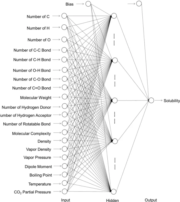
Fig. 1 Structure of the back-propagation neural network (BPNN) developed in this study, with the input, hidden, and output layers. The empty circles represent the neurons of the artificial neural network
(ANN) algorithmic architecture. The input and output layers, respec-tively, represent the input and output variables of the model. Each neuron interconnects with all the neurons in the adjacent layers
1400 Environmental Chemistry Letters (2019) 17:1397–1404
1 3
of input neurons, N is the number of hidden neurons, and Y is the number of output neurons.
A schematic picture of the artificial neural network (ANN) in the form of a back-propagation neural network (BPNN) is depicted in Fig. 1, with the input, hidden, and output layers. Each circle (neuron) in the input layer rep-resents an independent variable that has potential relation-ships with the output. The circle (neuron) in the output layer represents the dependent variable, e.g., CO2 solubil-ity. Each neuron connects to all the other neurons in the layer nearby in the form of weights. The training of an ANN is, essentially, the optimization of the weight values. A sigmoid function was used as the activation function that transfers the input data and weights into the output values.
Being different from BPNN, GRNN has a fixed network architecture with the Gaussian as the activation function (Li et al. 2015). More algorithmic principles of the BPNN and GRNN can be found in Hornik et al. (1989), Specht (1991) and Svozil et al. (1997). In order to compare the linear and nonlinear fitting results, multiple linear regressions (MLR) were also performed and compared with ANNs.
The modeling processes include the training and testing of the model. For each training and testing, all data were firstly shuffled and then split into the training and testing sets. The training sets were used for the data fitting, while the testing sets were used to validate the predictive capacity of the model. To evaluate the model performance, previous studies have shown that compared with a tedious cross-val-idation method (Browne 2000), a sensitivity test could also be more valuable, with significantly less time-consumption
and less computational costs (Li et al. 2017a, b; Maeda
2018). Therefore, in our study, we used sensitivity tests to evaluate our model. To perform a sensitivity test, multiple training and testing processes were repeated with randomly shuffled data before each modeling. Then, the average root-mean-squared error (RMSE) of the testing set can be acquired. For all the modeling processes in this study, the average RMSE was used as the loss function to evaluate the accuracy of the model (Li et al. 2017a):
where n represents the number of data in the training or testing set, Ai represents the actual value, and Pi represents
the predicted value. In order to define the optimized network architecture, 624 data from Gui et al. (2011) were used for evaluating the RMSEs of the modeling with varying num-bers of hidden neurons and hidden layers, with the reason that experiments done by the same literature would lead to less noises.
Data collection
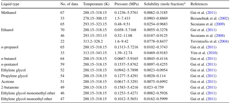
CO2 solubility, in the form of mole fraction, in 11 absor-bent types, was collected from the experimental literature (Bezanehtak et al. 2002; Tsivintzelis et al. 2004; Secuianu et al. 2008, 2009; Yim et al. 2010; Gui et al. 2011). Their descriptive statistics are listed in Table 1. In the machine learning modeling, 823 data were used. From Table 1, all (1) RMSE = � ∑n i=1�Pi− Ai �2 n ,
Table 1 Data range of experimental conditions and CO2 solubility in physical solvents
a Mole fraction (x) = n g n
g+nl (ng and nl denote the amounts of gas and solvent, respectively)
Liquid type No. of data Temperature (K) Pressure (MPa) Solubility (mole fraction)a References
Methanol 67 288.15–318.15 0.1236–5.5761 0.0062–0.3185 Gui et al. (2011) 33 278.15–308.15 1.5–7.433 0.0903–0.8869 Bezanehtak et al. (2002) 65 293.15–323.15 0.48–9.51 0.0254–0.9683 Secuianu et al. (2009) Ethanol 70 288.15–318.15 0.058–5.7168 0.0055–0.3278 Gui et al. (2011)
46 293.15–353.15 0.52–11.08 0.0187–0.9125 Secuianu et al. (2008) 22 313.2–328.2 1.6–9.42 0.0778–0.8437 Tsivintzelis et al. (2004)
n-propanol 65 288.15–318.15 0.1313–5.7216 0.0102–0.3743 Gui et al. (2011)
33 313.15–343.15 1.39–12.74 0.0469–0.9183 Yim et al. (2010)
n-butanol 64 288.15–318.15 0.0667–5.9165 0.0045–0.4116 Gui et al. (2011)
n-pentanol 59 288.15–318.15 0.1537–5.8762 0.0097–0.4255 Gui et al. (2011)
Ethylene glycol 52 288.15–318.15 0.0942–5.7898 0.0023–0.0954 Gui et al. (2011) Propylene glycol 54 288.15–318.15 0.1277–5.4291 0.0028–0.114 Gui et al. (2011) Acetone 51 288.15–318.15 0.0617–5.3291 0.0075–0.6992 Gui et al. (2011) 2-butanone 49 288.15–318.15 0.1583–5.4216 0.023–0.759 Gui et al. (2011) Ethylene glycol monomethyl ether 46 288.15–318.15 0.1253–5.4271 0.0082–0.5926 Gui et al. (2011) Ethylene glycol monoethyl ether 47 288.15–318.15 0.1012–5.5651 0.0162–0.5999 Gui et al. (2011)
these variables are quite diverse, which is well suited for the training of a generalized machine learning model.
Results and discussion
In this section, we show the modeling results of the artifi-cial neural network (ANN) for predicting the CO2
solubil-ity. Predictive performances of different ANN algorithmic architectures and different models are compared.
Model training and testing
To test the descriptors developed in these studies, we devel-oped a back-propagation neural network (BPNN), a gen-eral regression neural network (GRNN), and multiple lin-ear regression (MLR), then we compared their accuracies (Figs. 2, 3). For BPNN, the best network architecture with minimized root-mean-squared errors (RMSE) must be found prior in comparison with other machine learning algorithms (Maeda 2018). Since GRNN has a fixed network architec-ture, only one type of GRNN was developed in this study.
To define the optimized BPNN architecture, the BPNNs with one and two hidden layers were respectively exam-ined. For each specific network architecture, ten multiple training and testing processes, with randomly shuffled data for each time, were performed and the average RMSEs in the testing set were calculated for each architecture.
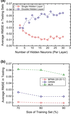
Results show that for the network with one hidden layer, the average testing RMSE generally decreases first with the increase in hidden neurons, while it increases after the hidden neuron is larger than 20 (Fig. 2a, red points). This indicates that before the hidden neuron reaches 20, there were generally under-fitting of the data, while after that there would be over-fitting, according to Tetko et al. (1995).
Concerning BPNN with two hidden layers, it can be clearly seen that all the tested architectures yield high aver-age testing RMSEs (Fig. 2a, blue points), indicating an over-fitting phenomenon. With this evaluation, it can be concluded that with our new input descriptors and the lit-erature database, BPNN with a 20-20-1 architecture has the minimized error. This suggests that 20-20-1 is a good net-work architecture. Though the number of hidden neurons is relatively large, it fulfills the empirical machine learning theory that with relatively large input data, the number of hidden neuron should also be increased in order to provide more weights to construct the complicated nonlinear rela-tionships between the independent and dependent variables. To evaluate how many training data could lead to a good predictive model, we compared the BPNN (20-20-1) with GRNN and MLR. Sensitivity tests were performed in these
three models, with the training percentages of 70%, 80%, and 90% (Fig. 2b). For each training and testing process, all the data were shuffled and then split into the training and testing sets before modeling.
Figure 2b shows the results of the average RMSEs in test-ing sets after sensitivity tests. Each data point was the aver-aged RMSE in the testing set from ten repeated training pro-cesses. Results reveal that the BPNN (20-20-1) outperforms the GRNN and MLR, having significantly lower average RMSEs in the three training percentages. Compared with GRNN, BPNN in this case has much better performance
0 5 10 15 20 25 30 35 0.00 0.01 0.02 0.03 0.04 0.05 0.06 0.07
Average RMSE in Testing Sets
Number of Hidden Neurons (Per Layer)
Single Hidden Layer Double Hidden Layer
(a) 70 80 90 0.01 0.02 0.03 0.04 0.05 0.06 0.07 (b)
Average RMSE in Testing
Size of Training Set (%)
BPNN (20-20-1) GRNN MLR
Fig. 2 a Average root-mean-squared errors (RMSEs) of the testing
sets with different back-propagation neural network (BPNN) hid-den architectures. Red circles represent the network with one hidhid-den layer, with the network architecture of 20-N-1, where N represents the number of hidden neurons. Blue squares represent the BPNN with two hidden layers, with the network architecture of 20-N–N-1. Each point is the average testing RMSE after ten training and test-ing processes with shuffled data. Lower average RMSE of the model indicates a model with better predictive accuracy, such as the single hidden layer model (red data). b RMSEs of back-propagation neural network with a BPNN (20-20-1), general regression neural network (GRNN), and multiple linear regression (MLR) for the prediction of CO2 solubility with three sizes of training data. Each point represents the average testing RMSE of ten repeated modeling processes with randomly shuffled data
1402 Environmental Chemistry Letters (2019) 17:1397–1404
1 3
in capturing the nonlinear relationships between the input and output data. Also, it is expected that BPNN would have better extrapolation predictive capacity than GRNN since GRNN is mainly designed for interpolation with a kernel-based algorithm. Noteworthy, although GRNN has much faster convergence speed when training with a suitable data size (Li and Zhang 2018), the BPNN should still be used in this case, to guarantee the predictive accuracy of this model.
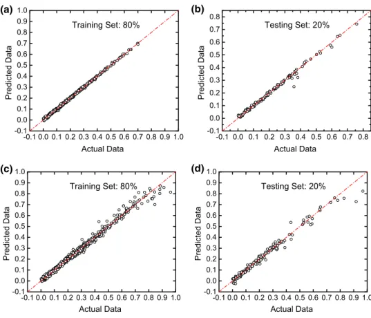
To compare the predicted and actual data in both the train-ing and testtrain-ing sets, selected representative results trained and tested from the data provided by Gui et al. (2011) are shown in Fig. 3a, b. Results show that with a larger training set, the testing set tends to have higher accuracy with data points close to the y = x diagonal. This indicates that larger training sets could help to more precisely capture the rela-tionships between the chemoinformatics-based descriptors and the CO2 solubility in physical solvents. To expand the model with larger databases, experimental data from other studies were also added to the training and testing databases, with totally 823 experimental data groups (Table 1). Similar training and testing evaluation processes show that though the predictive accuracy slightly decreases due to the data noise in experiments done by different research groups, the predictive performances of the model are still guaranteed (Fig. 3c, d).
Conclusion
We designed a new descriptor representation that includes structural and bond information, thermodynamic properties of solvent, and experimental operating conditions as the model input variables, to predict CO2 solubility in physi-cal solvents. A model with a back-propagation algorithm trained from 823 experimental data of alcohol, ketone, and ether solvents shows good accuracy for the prediction of CO2 solubility. Our comparative analysis shows that a back-propagation neural network (BPNN) with an algorithmic architecture of 20-20-1 can perform minimized errors, out-performing the general regression neural network (GRNN) and linear regression models. This study shows that with a set of reasonable chemoinformatics-based descriptors, CO2
solubility could be precisely predicted when being dissolved in physical solvents under varying experimental conditions.
Moreover, we show that a machine learning model can be used to predict the performance of a CO2 absorbent and
to optimize its experimental operating conditions. With the future demand of big data analysis, it is expected that such a model with larger and more diverse experimental database could help to meet the demand with more types of organic solvents. It is also expected that a well-trained model with these descriptors could also predict the CO2 solubility in
Fig. 3 Selected typical (a) training and (b) testing results of predicted values versus actual values trained and tested from 624 data groups extracted from Gui et al. (2011). Selected typical (c) training and (d) test-ing results of predicted values versus actual values trained and tested from 823 data. The percentages of training and testing sets are 80% and 20%, respectively. Results with other training and testing percentages can be found in Figures S1 and S2. The diagonal dashed line represents the line of y = x. The data point which is close to the diagonal dashed line indicates a good prediction -0.1 0.0 0.1 0.2 0.3 0.4 0.5 0.6 0.7 0.8 0.9 1.0 -0.1 0.0 0.1 0.2 0.3 0.4 0.5 0.6 0.7 0.8 0.9 1.0 Predicted Dat a Actual Data (a) Training Set: 80% -0.1 0.0 0.1 0.2 0.3 0.4 0.5 0.6 0.7 0.8 -0.1 0.0 0.1 0.2 0.3 0.4 0.5 0.6 0.7 0.8 Predicted Dat a Actual Data (b) Testing Set: 20% -0.1 0.0 0.1 0.2 0.3 0.4 0.5 0.6 0.7 0.8 0.9 1.0 -0.1 0.0 0.1 0.2 0.3 0.4 0.5 0.6 0.7 0.8 0.9 1.0 Predicted Dat a Actual Data (c) Training Set: 80% -0.1 0.0 0.1 0.2 0.3 0.4 0.5 0.6 0.7 0.8 0.9 1.0 -0.1 0.0 0.1 0.2 0.3 0.4 0.5 0.6 0.7 0.8 0.9 1.0 Predicted Dat a Actual Data (d) Testing Set: 20%
other more complicated organic solvents. It should be noted that in this study, we selected the structural and bond infor-mation, thermodynamic properties, and experimental condi-tions as the model input data. It is also expected that some other information, e.g, other thermodynamic properties of the organic solvent that have potential correlations with CO2
solubility, could also help to further improve the model com-prehensiveness and applicability when dealing with more types of complicated organic solvents.
References
Aaron D, Tsouris C (2005) Separation of CO2 from flue gas: a review.
Sep Sci Technol 40:321–348. https ://doi.org/10.1081/SS-20004 2244
Adzic RR, Zhang J, Sasaki K et al (2007) Platinum monolayer fuel cell electrocatalysts. Top Catal 46:249–262. https ://doi.org/10.1007/ s1124 4-007-9003-x
Aeshala LM, Uppaluri RG, Verma A (2013) Effect of cationic and anionic solid polymer electrolyte on direct electrochemical reduc-tion of gaseous CO2 to fuel. J CO2 Util 3(4):49–55. https ://doi.
org/10.1016/j.jcou.2013.09.004
Behler J, Parrinello M (2007) Generalized neural-network representa-tion of high-dimensional potential-energy surfaces. Phys Rev Lett.
https ://doi.org/10.1103/physr evlet t.98.14640 1
Bezanehtak K, Combes GB, Dehghani F et al (2002) Vapor-liquid equi-librium for binary systems of carbon dioxide + methanol, hydro-gen + methanol, and hydrohydro-gen + carbon dioxide at high pressures. J Chem Eng Data 47:161–168. https ://doi.org/10.1021/je010 122m
Böttcher T (2016) An additive definition of molecular complexity. J Chem Inf Model. https ://doi.org/10.1021/acs.jcim.5b007 23
Browne MW (2000) Cross-validation methods. J Math Psychol 44:108–132. https ://doi.org/10.1006/jmps.1999.1279
Dai C, Wei W, Lei Z, Li C, Chen B (2015) Absorption of CO2 with methanol and ionic liquid mixture at low temperatures. Fluid Phase Equilib 391:9–17. https ://doi.org/10.1016/j.fluid .2015.02.002
Duan Z, Sun R (2003) An improved model calculating CO2 solubil-ity in pure water and aqueous NaCl solutions from 273 to 533 K and from 0 to 2000 bar. Chem Geol 193:257–271. https ://doi. org/10.1016/S0009 -2541(02)00263 -2
Gui X, Tang Z, Fei W (2011) Solubility of CO2 in alcohols, glycols, ethers, and ketones at high pressures from (288.15 to 318.15) K. J Chem Eng Data 56:2420–2429. https ://doi.org/10.1021/je101 344v
Hornik K, Stinchcombe M, White H (1989) Multilayer feedforward networks are universal approximators. Neural Netw 2:359–366.
https ://doi.org/10.1016/0893-6080(89)90020 -8
Koytsoumpa EI, Bergins C, Kakaras E (2018) The CO2 economy: review of CO2 capture and reuse technologies. J Supercrit Fluids
132:3–16. https ://doi.org/10.1016/j.supfl u.2017.07.029
Krupa SV, Kickert RN (1993) The greenhouse effect: the impacts of carbon dioxide (CO2), ultraviolet-B (UV-B) radiation and ozone
(O3) on vegetation (crops). Vegetatio 104–105:223–238. https ://
doi.org/10.1007/BF000 48155
Li H, Henkelman GA (2017) Dehydrogenation selectivity of ethanol on close-packed transition metal surfaces: a computational study of monometallic, Pd/Au, and Rh/Au catalysts. J Phys Chem C 121:27504–27510. https ://doi.org/10.1021/acs.jpcc.7b099 53
Li H, Zhang Z (2018) Mining the intrinsic trends of CO2 solubil-ity in blended solutions. J CO2 Util 26:496–502. https ://doi.
org/10.1016/j.jcou.2018.06.008
Li B, Duan Y, Luebke D, Morreale B (2013) Advances in CO2 capture
technology: a patent review. Appl Energy 102:1439–1447. https ://doi.org/10.1016/j.apene rgy.2012.09.009
Li H, Chen F, Cheng K et al (2015) Prediction of zeta potential of decomposed peat via machine learning: comparative study of sup-port vector machine and artificial neural networks. Int J Electro-chem Sci 10:6044–6056
Li H, Liu Z, Liu K, Zhang Z (2017a) Predictive power of machine learning for optimizing solar water heater performance: the poten-tial application of high-throughput screening. Int J Photoenergy 1:2. https ://doi.org/10.1155/2017/41942 51
Li H, Zhang Z, Liu Z (2017b) Application of artificial neural networks for catalysis: a review. Catalysts 7:306. https ://doi.org/10.3390/ catal 71003 06
Li H, Evans EJ, Mullins CB, Henkelman G (2018a) Ethanol decompo-sition on Pd-Au alloy catalysts. J Phys Chem C 122:22024–22032.
https ://doi.org/10.1021/acs.jpcc.8b081 50
Li H, Luo L, Kunal P et al (2018b) Oxygen reduction reaction on clas-sically immiscible bimetallics: a case study of RhAu. J Phys Chem C 122:2712–2716. https ://doi.org/10.1021/acs.jpcc.7b109 74
Li H, Shin K, Henkelman G (2018c) Effects of ensembles, ligand, and strain on adsorbate binding to alloy surfaces. J Chem Phys 149:174705. https ://doi.org/10.1063/1.50538 94
Liu P, Lin H, Yang Y et al (2014) New insights into thermal decom-position of polycyclic aromatic hydrocarbon oxyradicals. J Phys Chem A 118:11337–11345. https ://doi.org/10.1021/jp510 498j
Liu P, Li Z, Roberts WL (2018a) The growth of PAHs and soot in the post-flame region. Proc Combust Inst 000:1–8. https ://doi. org/10.1016/j.proci .2018.05.047
Liu P, Zhang Y, Wang L et al (2018b) Chemical mechanism of exhaust gas recirculation on polycyclic aromatic hydrocarbons formation based on laser-induced fluorescence measurement. Energy Fuels 32:7112–7124. https ://doi.org/10.1021/acs.energ yfuel s.8b004 22
Maeda T (2018) Technical note: how to rationally compare the per-formances of different machine learning models? PeerJ Preprints 6:e26714v1. https ://doi.org/10.7287/peerj .prepr ints.26714 v1
Murad S, Gupta S (2000) A simple molecular dynamics simulation for calculating Henry’s constant and solubility of gases in liq-uids. Chem Phys Lett 319:60–64. https ://doi.org/10.1016/S0009 -2614(00)00085 -3
Nawi NM, Khan A, Rehman MZ (2013) A new back-propagation neural network optimized. Iccsa 2013:413–426. https ://doi. org/10.1007/978-3-642-39637 -3
Padilla M, Baturina O, Gordon JP, Artyushkova K, Atanassov P, Serov A (2017) Selective CO2 electroreduction to C2H4 on porous
Cu films synthesized by sacrificial support method. J CO2 Util
19:137–145. https ://doi.org/10.1016/j.jcou.2017.03.006
Park J-H, Jun C-H (2013) Multivariate process control chart for con-trolling the false discovery rate. Ind Eng Manag Syst 11:385–389.
https ://doi.org/10.7232/iems.2012.11.4.385
Park J, Jun CH (2015) A new multivariate EWMA control chart via multiple testing. J Process Control. https ://doi.org/10.1016/j.jproc ont.2015.01.007
Paul S, Ghoshal AK, Mandal B (2008) Theoretical studies on separa-tion of CO2 by single and blended aqueous alkanolamine solvents
in flat sheet membrane contactor (FSMC). Chem Eng J 144:352– 360. https ://doi.org/10.1016/j.cej.2008.01.036
Secuianu C, Feroiu V, Geană D (2008) Phase behavior for carbon diox-ide + ethanol system: experimental measurements and modeling with a cubic equation of state. J Supercrit Fluids 47:109–116.
https ://doi.org/10.1016/j.supfl u.2008.08.004
Secuianu C, Feroiu V, Geanǎ D (2009) Phase equilibria experi-ments and calculations for carbon dioxide + methanol binary system. Cent Eur J Chem 7:1–7. https ://doi.org/10.2478/s1153 2-008-0085-5
1404 Environmental Chemistry Letters (2019) 17:1397–1404
1 3
Singh S, Gautam RK, Malik K, Verma A (2017) Ag-Co bimetallic catalyst for electrochemical reduction of CO2 to value added
products. J CO2 Util 18:139–146. https ://doi.org/10.1016/j.
jcou.2017.01.022
Specht DF (1991) A general regression neural network. IEEE Trans Neural Netw 2:568–576. https ://doi.org/10.1109/72.97934
Svozil D, Kvasnicka V, Pospichal J (1997) Introduction to multi-layer feed-forward neural networks. Chemom Intell Lab Syst 39:43–62.
https ://doi.org/10.1016/S0169 -7439(97)00061 -0
Tetko IV, Livingstone DJ, Luik AI (1995) Neural network studies. 1. Comparison of overfitting and overtraining. J Chem Inf Comput Sci 35:826–833. https ://doi.org/10.1021/ci000 27a00 6
Tontiwachwuthikul P, Meisen A, Lim CJ (1992) CO2 absorption by
NaOH, monoethanolamine and 2-amino-2-methyl-1-propanol solutions in a packed column. Chem Eng Sci 47:381–390. https ://doi.org/10.1016/0009-2509(92)80028 -B
Tsivintzelis I, Missopolinou D, Kalogiannis K, Panayiotou C (2004) Phase compositions and saturated densities for the binary systems of carbon dioxide with ethanol and dichloromethane. Fluid Phase Equilib 224:89–96. https ://doi.org/10.1016/j.fluid .2004.06.046
Wang Y, Xiao J, Suzek TO, Zhang J, Wang J, Bryant SH (2009) PubChem: a public information system for analyzing bioactivi-ties of small molecules. Nucleic Acids Res 37:W623–W633. https ://doi.org/10.1093/nar/gkp45 6
Wei CC, Puxty G, Feron P (2014) Amino acid salts for CO2 capture
at flue gas temperatures. Chem Eng Sci 107:218–226. https ://doi. org/10.1016/j.ces.2013.11.034
Yim JH, Jung YG, Lim JS (2010) Vapor-liquid equilibria of carbon dioxide + n-propanol at elevated pressure. Korean J Chem Eng 27:284–288. https ://doi.org/10.1007/s1181 4-009-0342-0
Yu CH, Huang CH, Tan CS (2012) A review of CO2 capture by
absorp-tion and adsorpabsorp-tion. Aerosol Air Qual Res 12:745–769. https :// doi.org/10.4209/aaqr.2012.05.0132
Zhang G, Eddy Patuwo B, Hu MY (1998) Forecasting with artificial neural networks. Int J Forecast 14:35–62. https ://doi.org/10.1016/ s0169 -2070(97)00044 -7
Zhang Z, Chen F, Rezakazemi M, Zhang W, Lu C, Chang H, Quan X (2018a) Modeling of a CO2-piperazine-membrane absorption
sys-tem. Chem Eng Res Des 131:375–384. https ://doi.org/10.1016/j. cherd .2017.11.024
Zhang Z, Li H, Chang H, Pan Z, Luo X (2018b) Machine learn-ing predictive framework for CO2 thermodynamic properties
in solution. J CO2 Util 26:152–159. https ://doi.org/10.1016/j.
jcou.2018.04.025
Zhang Z, Li Y, Zhang W, Wang J, Soltanian MR, Olabi AG (2018c) Effectiveness of amino acid salt solutions in capturing CO2: a
review. Renew Sustain Energy Rev 98:179–188. https ://doi. org/10.1016/j.rser.2018.09.019
Publisher’s Note Springer Nature remains neutral with regard to jurisdictional claims in published maps and institutional affiliations.