Decarbonization of power systems : analyzing different technological pathways

(1)

Decarbonization of Power Systems: Analyzing Different

Technological Pathways

by

Nestor A. Sepulveda

B.S., Naval Electrical Engineering, Naval Polytechnic Academy, Chile, 2010 Submitted to the Department of Nuclear Science and Engineering &

Institute for Data, Systems, and Society

in partial fulfillment of the requirements for the degree of

Master of Science in Nuclear Science and Engineering & Master of Science in Technology and Policy

at the

MASSACHUSETTS INSTITUTE OF TECHNOLOGY September 2016

c

Author . . . . Department of Nuclear Science and Engineering &

Institute for Data, Systems, and Society Aug 07, 2016 Certified by . . . . Richard K. Lester Associate Provost Japan Steel Industry Professor of Nuclear Science and Engineering Thesis Supervisor Certified by . . . . Charles W. Forsberg Principal Research Scientist Department of Nuclear Science and Engineering Thesis Supervisor Certified by . . . . Fernando J. de Sisternes Energy Specialist, The World Bank Research Affiliate, MIT Center for Energy and Environmental Policy Research Thesis Supervisor Accepted by . . . .

Ju Li Battelle Energy Alliance Professor of Nuclear Science and Engineering Chair, Department Committee on Graduate Students Accepted by . . . .

Munther A. Dahleh William A. Coolidge Professor of Electrical Engineering and Computer Science Director, Institute for Data, Systems, and Society

(2)

(3)

To my wife and my parents Maria Soledad, Carlos y Patricia

(4)

(5)

Decarbonization of Power Systems: Analyzing Different Technological Pathways

by

Nestor A. Sepulveda

Submitted to the Department of Nuclear Science and Engineering & Institute for Data, Systems, and Society

on Aug 07, 2016, in partial fulfillment of the requirements for the degree of

Master of Science in Nuclear Science and Engineering & Master of Science in Technology and Policy

Abstract

Climate change poses a major challenge to society. Different sectors of society will need to respond in different ways; for the power sector, the response will require the aggressive reduction of CO2

emissions to near zero by 2050. There is no unique pathway for achieving a given level of decar-bonization, and different pathways will require greater or lesser resources. In general, as the degree of carbon mitigation increases, each additional unit of reduction will become more expensive. The world has limited resources, as do national economies. Thus, whether the solution to decarboniza-tion is achieved through markets or through centralized planning, the soludecarboniza-tion should be the one that maximizes society’s welfare, i.e., that achieves the goal at minimum cost for society.

This thesis explores the potential cost implications of different decarbonization pathways for the electricity generation mix in the year 2050. The impacts of different CO2 reduction targets and

technological choices on the cost of decarbonization are compared. The average price of electricity is used as a metric for the cost of decarbonization to society. An important requirement of the analysis is to take account of changes in the expected cost of existing technologies over this period, as well as the possibility that new technologies will become available. This research takes a systemic view, including a detailed representation of the interactions between different types of power system technologies, taking into consideration the synergies and limitations that each asset class creates and/or imposes on others.

To explore the impact of differences in system characteristics, two different U.S. power systems are analyzed: New England’s power system and the Texas power system. These differ significantly in their demand profiles and in the availability of renewable resources. Cost estimates developed by the International Energy Agency and the Nuclear Energy Agency for 2020 are used as input parameters for the analysis. Uncertainty in cost estimates is addressed by a comprehensive sensitivity analysis on future cost reductions for renewables and storage systems, as well as future cost increases for nuclear technologies. Additionally, to account in part for the likelihood of future changes in the pool of available technological options, two new supply-side technologies currently under development are included in the analysis, as are new capabilities for managing demand-side resources.

A novel long-term generation investment model, GenX, has been developed to determine the minimum cost generation mix subject to various emissions constraints and different technological pathways. GenX is a capacity expansion model with clustered unit commitment constraints whose

(6)

main features include: 1) the ability to evaluate the impact of operating constraints with hourly resolution on investment decisions and on total generation cost; 2) the ability to account for the chronological variability of demand and renewable output, and correlations between the two; and 3) the ability to decide on power plant investments and operation at the individual plant level. Each technology is characterized by a particular set of operational and economic parameters. Ad-ditionally, GenX is capable of modeling new technological concepts –advanced nuclear (Generation IV) and heat storage– which would support interactions between electricity and heat markets. The model is implemented in the Julia language and has been used to simulate 560 different decar-bonization/technology scenarios.

Key results include: (1) the importance for minimizing the cost of decarbonization of having a diversity of technological options with a range of technical and economic attributes; more specifi-cally, (2) the central importance of having dispatchable low-carbon resources, such as nuclear power or carbon capture and sequestration systems. For example, when dispatchable low-carbon technolo-gies are not available, the cost of achieving deep decarbonization goals is shown to triple in power systems such as New England’s with lower renewables potential, and to double even in a Texas-like system with higher renewables potential; and (3) the great potential of new technological con-cepts for simultaneously reducing CO2 emissions and decreasing the cost of electricity considerably.

An important policy implication of this work is the need to shift from technology-specific support mechanisms for decarbonization (e.g. renewable portfolio standards) to general low-carbon support mechanisms that will allow for competition between and adaptation of low-carbon technologies.

The methodology developed in this research supports two important new capabilities for policy makers: (1) the ability to calculate the extra cost associated with dispensing with specific technolog-ical options –such as nuclear power– will enable improved cost-benefit analysis of policies directed towards specific technologies; (2) the ability to model the potential impact of new technological concepts on the cost of decarbonization will help to optimize the allocation of R&D resources with respect to their potential contribution to reducing CO2 abatement costs.

Thesis Supervisor: Richard K. Lester Title: Associate Provost

Japan Steel Industry Professor of Nuclear Science and Engineering

Thesis Supervisor: Charles W. Forsberg

Title: Principal Research Scientist Department of Nuclear Science and Engineering

Thesis Supervisor: Fernando J. de Sisternes Title: Energy Specialist, The World Bank

(7)

Acknowledgments

This thesis would have never been possible without the support and guidance from many people. By the time I write this words, one month has passed since I underwent open heart surgery; I am thankful to God for being able to write them.

I would like to thank my thesis supervisors, Professor Richard Lester, Dr. Charles Forsberg, and Dr. Fernando de Sisternes, for their guidance, critical insight and invaluable feedback during this research project; and for finding time in their busy schedules to meet with me. Special thanks to Fernando, for being a great mentor, and for his friendship.

I am thankful to Professor R. Scott Kemp whose class inspired this research; and who challenged me to explore what at that time seemed an unexplored question. The work done for the term paper I wrote for his class “22.16” is the foundation stone of this work.

Special thanks to Jesse Jenkins who trusted on my abilities and work; and decided to join efforts to create something better than what each one alone would have done. We called that effort “GenX,” a model that is far more capable that what I have described in this thesis. I thank Jesse for sharing his expert knowledge, and for his friendship.

I would like to thank Miles Lubin, not only for developing JuMP –the main tool used in writing GenX– but also for helping me come to terms with the Julia Language and always being available for questions at the inception of the model.

More generally I would like to thank MIT, the department of Nuclear Science and Engineering (NSE), and the Technology and Policy Program (TPP) at the Institute for Data, Systems, and Society for having me during these two years. I learned a lot in contact with prestigious professors and awesome people from all around the world. I thank NSE faculty, for all they taught me, and the NSE staff for the work that they do. I have a special thought for Professor Michael W. Golay, my academic advisor. I would like to recognize the members of the TPP staff, Ed Ballo, Barbara DeLaBarre and Dr. Frank R. Field for the work that they do, for the great support they provide to students and for making TPP a great place. Special thanks to Frank for making sure I did not kill myself taking too many classes (I will miss our negotiations), and for helping me prepare for the surgery.

I am also especially grateful to my NSE classmates who helped me overcome the difficulties I faced during the first months of this incredible experience; and my TPP classmates for making my

(8)

time at MIT even more delightful.

I am indebted to the Chilean Navy, the institution that has funded my graduate studies, and that has trained and educated me. I am very grateful to Chile for the excellent education it provided to me.

I feel immensely grateful to the staff at the Boston Children’s Hospital who took good care of me before and after the surgery; allowing me to get back to work in record time to finish this thesis. Special thanks to Dr. Alexander Opotowsky, my cardiologist, and Dr. Pedro del Nido, my surgeon, for taking care of my condition with the greatest readiness.

Finally, I must express my very profound gratitude to my family. My parents who taught me the value of hard work, to never give up, and for their unconditional and unwavering support and love. My parents in-law for trusting me her daughter and for their unconditional help. To my wife for providing me with unfailing support, there are no words to convey the sense of gratitude I feel; you mean the world to me and I would have never made it without you. Thank you.

(9)

List of Figures

1-1 Wholesale short run energy pricing . . . 25

1-2 Market price duration curve and revenues expected by generators with and without price caps . . . 28

2-1 Temperature increase probability as function of CO2 concentrations by 2080-2100 . . 36

2-2 CO2 emissions trajectories for the energy sector . . . 37

2-3 CO2 emissions allowance for different world regions and for different mitigation tar-gets (blue) compared to BAU, baseline, scenario (yellow) . . . 38

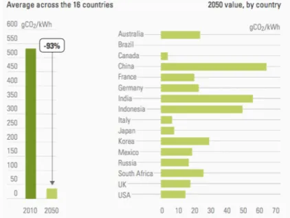
2-4 Average carbon intensity of electricity for 16 countries as a whole, 2010 and 2050. Carbon intensity of electricity in 2050, for individual countries . . . 39

2-5 Nuclear Air-Brayton Combined Cycle (NACC) . . . 41

2-6 Effect of Size on Cost of Gas Turbine Combined Cycle Units . . . 43

2-7 FIRES allowing electricity-heat market interactions . . . 45

3-1 Unit Commitment Approaches . . . 68

4-1 Renewables’ Availability Duration Curves Regional Data. . . 87

4-2 Load Duration Curves Regional Data. . . 88

4-3 ISO-NE and ERCOT Heat Duration Curves. . . 89

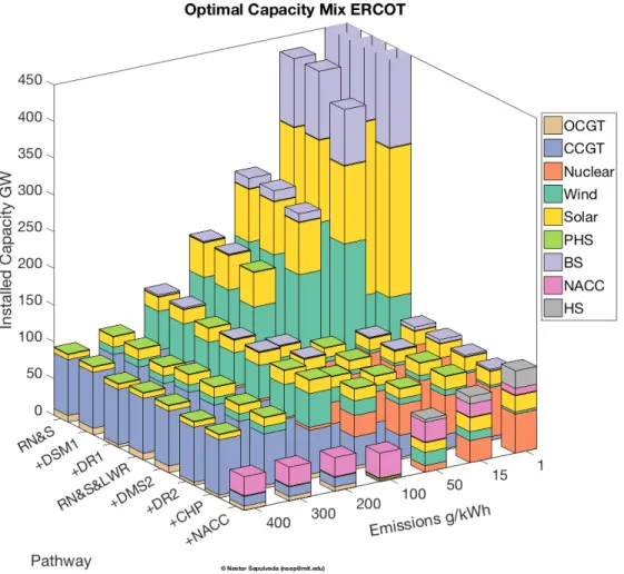
4-4 ERCOT’s optimal investment mix as function of pathways and emissions intensity targets. . . 93

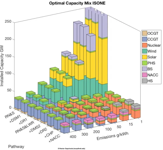
4-5 ISO-NE’s optimal investment mix as function of pathways and emissions intensity targets. . . 95

(14)

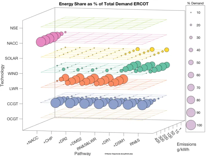
4-7 ISO’NE’s energy share as function of pathways and emissions intensity targets. . . . 99

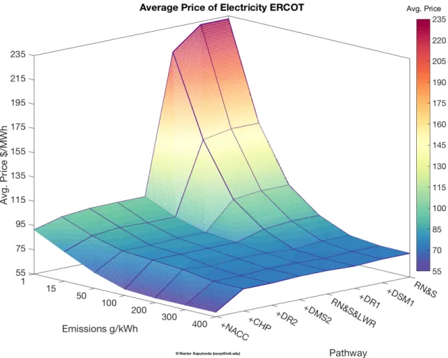
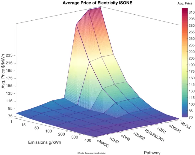
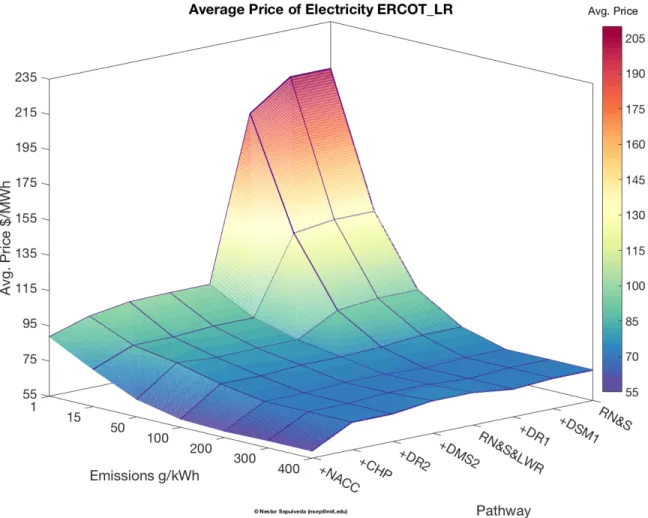
4-8 ERCOT’s average price of electricity as function of pathways and emissions intensity targets. . . 101

4-9 ISO-NE’s average price of electricity as function of pathways and emissions intensity targets. . . 102

4-10 ERCOT’s capacity mix (left axis) and average price of electricity (right axis) for specific CO2 targets. . . 105

4-11 ISO-NE’s capacity mix (left axis) and average price of electricity (right axis) for specific CO2 targets. . . 107

4-12 ERCOT average price of electricity for the different sensitivity analyses . . . 110

4-13 ERCOT capacity mix for the different sensitivity analyses . . . 111

4-14 ISO-NE average price of electricity for the different sensitivity analyses . . . 114

4-15 ISO-NE capacity mix for the different sensitivity analyses . . . 115

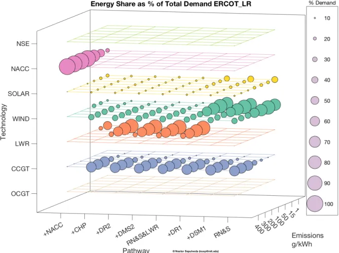
A-1 ERCOT’s optimal investment mix as function of pathways and emissions intensity targets, LR analysis. . . 126

A-2 ERCOT’s energy share as function of pathways and emissions intensity targets, LR analysis. . . 127

A-3 ERCOT’s average price of electricity as function of pathways and emissions intensity targets, LR analysis. . . 128

A-4 ERCOT’s capacity mix (left axis) and average price of electricity (right axis) for specific CO2 targets, LR analysis. . . 130

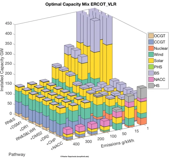
A-5 ERCOT’s optimal investment mix as function of pathways and emissions intensity targets, VLR analysis. . . 131

A-6 ERCOT’s energy share as function of pathways and emissions intensity targets, VLR analysis. . . 132

A-7 ERCOT’s average price of electricity as function of pathways and emissions intensity targets, VLR analysis. . . 133

A-8 ERCOT’s capacity mix (left axis) and average price of electricity (right axis) for specific CO2 targets, VLR analysis. . . 135

(15)

A-9 ERCOT’s optimal investment mix as function of pathways and emissions intensity targets, ELR analysis. . . 136 A-10 ERCOT’s energy share as function of pathways and emissions intensity targets, ELR

analysis. . . 137 A-11 ERCOT’s average price of electricity as function of pathways and emissions intensity

targets, ELR analysis. . . 138 A-12 ERCOT’s capacity mix (left axis) and average price of electricity (right axis) for

specific CO2 targets, ELR analysis. . . 140

A-13 ERCOT’s optimal investment mix as function of pathways and emissions intensity targets, HN analysis. . . 141 A-14 ERCOT’s energy share as function of pathways and emissions intensity targets, HN

analysis. . . 142 A-15 ERCOT’s average price of electricity as function of pathways and emissions intensity

targets, HN analysis. . . 143 A-16 ERCOT’s capacity mix (left axis) and average price of electricity (right axis) for

specific CO2 targets, HN analysis. . . 145

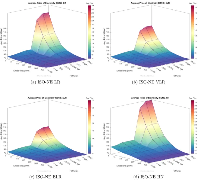
A-17 ISO-NE’s optimal investment mix as function of pathways and emissions intensity targets, LR analysis. . . 146 A-18 ISO-NE’s energy share as function of pathways and emissions intensity targets, LR

analysis. . . 147 A-19 ISO-NE’s average price of electricity as function of pathways and emissions intensity

targets, LR analysis. . . 148 A-20 ISO-NE’s capacity mix (left axis) and average price of electricity (right axis) for

specific CO2 targets, LR analysis. . . 150

A-21 ISO-NE’s optimal investment mix as function of pathways and emissions intensity targets, VLR analysis. . . 151 A-22 ISO-NE’s energy share as function of pathways and emissions intensity targets, VLR

analysis. . . 152 A-23 ISO-NE’s average price of electricity as function of pathways and emissions intensity

(16)

A-24 ISO-NE’s capacity mix (left axis) and average price of electricity (right axis) for

specific CO2 targets, VLR analysis. . . 155

A-25 ISO-NE’s optimal investment mix as function of pathways and emissions intensity targets, ELR analysis. . . 156

A-26 ISO-NE’s energy share as function of pathways and emissions intensity targets, ELR analysis. . . 157

A-27 ISO-NE’s average price of electricity as function of pathways and emissions intensity targets, ELR analysis. . . 158

A-28 ISO-NE’s capacity mix (left axis) and average price of electricity (right axis) for specific CO2 targets, ELR analysis. . . 160

A-29 ISO-NE’s optimal investment mix as function of pathways and emissions intensity targets, HN analysis. . . 161

A-30 ISO-NE’s energy share as function of pathways and emissions intensity targets, HN analysis. . . 162

A-31 ISO-NE’s average price of electricity as function of pathways and emissions intensity targets, HN analysis. . . 163

A-32 ISO-NE’s capacity mix (left axis) and average price of electricity (right axis) for specific CO2 targets, HN analysis. . . 165

B-1 ERCOT Demand Variability, Sample Summer Week. . . 168

B-2 ERCOT Demand Variability, Sample Winter Week. . . 169

B-3 ERCOT Solar Resource Variability, Sample Summer Week. . . 169

B-4 ERCOT Solar Resource Variability, Sample Winter Week. . . 170

B-5 ERCOT Wind Resource Variability, Sample Summer Week. . . 170

B-6 ERCOT Wind Resource Variability, Sample Winter Week. . . 171

B-7 ERCOT Heat Demand Variability, Sample Summer Week. . . 171

B-8 ERCOT Heat Demand Variability, Sample Winter Week. . . 172

B-9 ISO-NE Demand Variability, Sample Summer Week. . . 173

B-10 ISO-NE Demand Variability, Sample Winter Week. . . 174

B-11 ISO-NE Solar Resource Variability, Sample Summer Week. . . 174

(17)

B-13 ISO-NE Wind Resource Variability, Sample Summer Week. . . 175

B-14 ISO-NE Wind Resource Variability, Sample Winter Week. . . 176

B-15 ISO-NE Heat Demand Variability, Sample Summer Week. . . 176

B-16 ISO-NE Heat Demand Variability, Sample Winter Week. . . 177

C-1 ERCOT system sample operation pathway “+DR1” . . . 180

C-2 ERCOT system sample operation pathway “+DR2” . . . 181

C-3 ERCOT system sample operation pathway “+CHP” . . . 181

C-4 ERCOT system sample operation pathway “+NACC” . . . 182

C-5 ERCOT system sample operation, HN analysis, pathway “+DR1” . . . 183

C-6 ERCOT system sample operation, HN analysis, pathway “+DR2” . . . 184

C-7 ERCOT system sample operation, HN analysis, pathway “+CHP” . . . 184

C-8 ERCOT system sample operation, HN analysis, pathway “+NACC” . . . 185

C-9 ERCOT system sample operation, LR analysis, pathway “+DR1” . . . 186

C-10 ERCOT system sample operation, LR analysis, pathway “+DR2” . . . 187

C-11 ERCOT system sample operation, LR analysis, pathway “+CHP” . . . 187

C-12 ERCOT system sample operation, LR analysis, pathway “+NACC” . . . 188

C-13 ERCOT system sample operation, VLR analysis, pathway “+DR1” . . . 189

C-14 ERCOT system sample operation, VLR analysis, pathway “+DR2” . . . 190

C-15 ERCOT system sample operation, VLR analysis, pathway “+CHP” . . . 190

C-16 ERCOT system sample operation, VLR analysis, pathway “+NACC” . . . 191

C-17 ERCOT system sample operation, ELR analysis, pathway “+DR1” . . . 192

C-18 ERCOT system sample operation, ELR analysis, pathway “+DR2” . . . 193

C-19 ERCOT system sample operation, ELR analysis, pathway “+CHP” . . . 193

C-20 ERCOT system sample operation, ELR analysis, pathway “+NACC” . . . 194

C-21 ISONE system sample operation pathway “+DR1” . . . 195

C-22 ISONE system sample operation pathway “+DR2” . . . 196

C-23 ISONE system sample operation pathway “+CHP” . . . 196

C-24 ISONE system sample operation pathway “+NACC” . . . 197

C-25 ISONE system sample operation, HN analysis, pathway “+DR1” . . . 198

(18)

C-27 ISONE system sample operation, HN analysis, pathway “+CHP” . . . 199

C-28 ISONE system sample operation, HN analysis, pathway “+NACC” . . . 200

C-29 ISONE system sample operation, LR analysis, pathway “+DR1” . . . 201

C-30 ISONE system sample operation, LR analysis, pathway “+DR2” . . . 202

C-31 ISONE system sample operation, LR analysis, pathway “+CHP” . . . 202

C-32 ISONE system sample operation, LR analysis, pathway “+NACC” . . . 203

C-33 ISONE system sample operation, VLR analysis, pathway “+DR1” . . . 204

C-34 ISONE system sample operation, VLR analysis, pathway “+DR2” . . . 205

C-35 ISONE system sample operation, VLR analysis, pathway “+CHP” . . . 205

C-36 ISONE system sample operation, VLR analysis, pathway “+NACC” . . . 206

C-37 ISONE system sample operation, ELR analysis, pathway “+DR1” . . . 207

C-38 ISONE system sample operation, ELR analysis, pathway “+DR2” . . . 208

C-39 ISONE system sample operation, ELR analysis, pathway “+CHP” . . . 208

(19)

List of Tables

3.1 Model’s General Structure and Reference to Equations . . . 51

3.2 Model Indices and Sets . . . 52

3.3 Model Variables . . . 53

3.4 Model Parameters . . . 53

4.1 Case Construction, Technological Pathways and CO2 Targets combinations. . . 81

4.2 Investment Economical Parameters Different Technologies. . . 84

4.3 Operational Economical Parameters Different Technologies. . . 84

4.4 Operational Parameters Generation Technologies. . . 85

4.5 Operational Parameters Storage Technologies. . . 85

4.6 Operational Parameters Demand Side Resources. . . 86

4.7 Regional Data Characteristics. . . 88

(20)

(21)

Chapter 1

Introduction

1.1 Climate Change and Energy 2050

The objective of “deep decarbonization” refers to the progressive reduction of greenhouse gas (GHG) emissions to a level consistent with limiting the increase in the average global surface temperature to 2◦C or less relative to pre-industrial conditions. This objective derives from the scientific consensus that a continuation of recent trends in global greenhouse gas emissions poses an unacceptably high risk of dangerous anthropogenic interference with the climate system [1]. To avoid this risk will require that the world cuts net emissions of greenhouse gases (GHG) so that they approach zero between 2050 and 2075 [2].

A high level of commercial energy use, currently dominated by fossil fuels, is a common feature of all modern societies. Current patterns of settlement, industrial production, and mobility have co-evolved with today’s energy system. Achieving a deeply decarbonized global economy by mid-century will require profound changes in this system even as the world’s population and economic output continue to grow. At the most basic level, this entails two kinds of changes – making a much more efficient use of energy to provide goods and services, and deeply reducing the carbon emitted in supplying that energy – all while avoiding serious economic disruption.

As described in [3], there are a number of plausible technology pathways for achieving deep decarbonization in the U.S. economy. Though different, they all have certain key features in common. Across all technology pathways there are “three pillars” that must all be in place in order to reach the 2050 decarbonization goal: energy efficiency, decarbonization of electricity generation,

(22)

and electrification.:

1. Highly efficient end-use of energy. Energy intensity, a measure of the energy efficiency of a nation’s economy, expressed as units of energy use per unit of GDP, must decline by 70% between now and 2050, implying a 20% reduction in final energy use despite a forecast pop-ulation increase of 40% and a 166% increase in GDP.

2. Nearly complete decarbonization of electricity. The carbon intensity of electricity must be reduced by at least 97%, from more than 500 g CO2/kWh today to 15 g CO2/kWh or less in 2050.

3. Electrification where possible. The share of end-use energy coming directly from electricity or fuels produced from electricity, such as hydrogen, must increase from less than 20% in 2010 to over 50% in 2050, displacing direct use of fossil fuels.

These three pillars are interdependent. For example, despite the fact that improvements in energy efficiency will help to decrease overall energy consumption in some sectors, electrification in others will cause an increase in electricity consumption. The overall effect, as estimated by the different System Operators, will be a net increase of electricity use over the next 35 years.

For the electric power system, perhaps the most urgent message of these reports is that we are just one investment cycle away from 2050. Given the 30+ year lifetimes of electric power facilities, the power generation planned today and built tomorrow will still be operational in 2050. Hence, any generation investments made today must either be capable of operating together with future technology deployments as part of a carbon-constrained power system or risk becoming overly expensive, under-utilized, “stranded” investments.

1.2 Background of Wholesale Electricity Markets

1.2.1 From Regulated to Deregulated Markets

Specialized electricity transportation and the economies of scale characteristic of Electric Power Systems (EPS) made it possible to consider formation of the monopoly in electric power industry as most natural and probable. Spontaneous (uncontrolled or unorganized) electricity markets gradually became monopoly ones in the early twentieth century. After recognition of this process

(23)

and the monopoly electricity market advantages for economies of scale, the natural monopolies (vertically integrated companies) became institutionally legalized under state regulation across the globe. Under this regime, consumers’ prices for electricity produced by natural monopolies were fixed by the regulatory bodies at the level of average operational and investment costs of the company.

Some problems arose with this system, for example: (1) Cost-of-service regulation, i.e., inclusion of all expenditures of the companies in tariffs that were recognized by the regulatory body as necessary and sound. In this case, the company had no special incentives to enhance production efficiency and reduce capital expenditures for EPS expansion, i.e., creation of surplus capacity reserves up to 30-40% in some zones, since utility profitability was a function of investment[4]. (2) Along with the companies, the regulatory bodies bore responsibility for reliable electricity supply to consumers. Both were inclined, therefore, to have surplus generation capacities rather than optimal capacities; creating a “regulatory capture” failure, since the regulator was motivated by self-interest and therefore selected policies that would not have gained the support of an informed public, but that were supported by the regulated; increasing consumers’ prices and profitability of utilities[5].

The indicated disadvantages, the idea growing idea of opening markets and the increase in electricity tariffs in some countries due to “inefficient investments” (since every cost was trans-ferred to the consumers) gave rise to criticism of the regulated model in the late twentieth century and brought about proposals on restructuring the electric power industry with implementation of competition in the area of electricity generation (deregulated generation). The new competition was expected to replace the state regulation (minimizing institutional failure), enhance production efficiency, and lead to electricity price reduction.

Since the liberalization of electricity generation began in 1982 in Chile, many countries have decided to introduce competition in their electricity industry to achieve greater economic efficiency [6][7]. Research shows [8] that this process has reduced the costs of service and other inefficiencies associated with the monopolistic behavior of the traditional vertically integrated utility. Compe-tition is best achieved through markets where the commodity can be freely traded. Accordingly, liberalized electric power systems have established wholesale markets for electricity generation to let market forces decide on the price and quantity of electricity that is to be produced. In this

(24)

con-text, it is the role of the regulator to establish a robust set of market rules that ensures competition while guaranteeing the security of electricity supply [9].

1.2.2 Wholesale Electricity Market

Under liberalization, market agents are left with tasks that they can perform more efficiently than the central planner. Subject to the conditions of electricity wholesale markets, operating decisions are not taken by a central operator, but by individual agents who try to maximize their profits [9]. These agents also decide on individual power plant investments that build up the system’s electricity generation capacity. According to economic theory, under ideal conditions a remuneration scheme based only on the short-term marginal cost of the system would allow generators to recover both operation costs and capital costs –including amortization and a rate of return on investment[10], attracting enough investors to build an adequate level of generating capacity.

A well functioning perfectly competitive wholesale electricity market will operate in one of two different states throughout the year. During regular operating conditions (State 1), market clearing prices for energy are equal to the marginal cost of the most expensive generating unit (i.e., typically, the one with the highest variable cost) that clears supply and demand at each point in time. In the case of wholesale electricity supply, this price is the marginal cost of producing a little more or a little less energy from the generating unit on the margin in the bid-based merit order system. Fig. 1-1a depicts the spot market demand for electricity and the competitive supply curve for electricity under typical operating conditions (State 1). Infra-marginal generating units earn net revenues that contribute to the recovery of their fixed operating and capital costs whenever the market clearing price exceeds their own marginal generation costs [9][6].

The second wholesale market state (State 2) is associated with a relatively small number of hours each year during which there is excess demand at a wholesale price that is equal to the marginal production cost of the last increment of generating capacity that can physically be made available on the network to supply energy (maximum available capacity). In this case, the market must be cleared, theoretically, “on the demand side”. That is, consumers bidding to obtain energy would bid prices up to a higher level reflecting the value that consumers place on consuming less electricity as demand is reduced to match the limited supply available in the market. In other words, the Value of Lost Load (VOLL) is the amount that customers of electricity would be willing

(25)

(a) State 1 pricing

(b) State 2 pricing

Figure 1-1: Wholesale short run energy pricing [6]

to pay to avoid a disruption in their electricity service. This second state is depicted in Fig. 1-1b; the area labeled Rmc represents the revenues that would be earned by infra-marginal generators if

the wholesale price is equal to the marginal generating cost of the least efficient generator on the system required to clear the market. The area labeled Rsreflects the additional “scarcity revenues”

from allowing prices to rise high enough to ration scarce capacity on the demand side to balance supply and demand. We refer to this as “shortage” condition or “scarcity hours”[9][6].

Under shortage conditions the competitive market clearing price of energy will now be higher than the marginal cost of supplying the last available increment of energy from generating capacity available in the network, reflecting the high opportunity cost (VOLL) that consumers place on

(26)

reducing consumption. All generating units actually supplying energy in the spot market during shortage conditions would earn substantial “scarcity rents.” These scarcity rents in turn help to recover the fixed capital and operating costs of all generating facilities and, in particular, of those generating units that only operate during peak hours.

In a hypothetical well-functioning competitive electricity market, price signals for energy bought and sold in the market not only induce the right amount of generating capacity, but also the right mix of generating technologies. Baseload plants –typically nuclear and coal power plants– will operate most of the time recovering their investment cost whenever not operating at the margin. Intermediate load plants –e.g., gas-fueled power plants– will typically operate for 20% to 50% of the hours during the year recovering their capital cost whenever they are infra-marginal. Finally, peaking plants –e.g., open cycle gas turbines or oil-fueled generators– are expected to operate from a few hours per year up to (say) 20% of the hours during the year, recovering their investment capital only during the hours of shortage.

The system described above, if operating optimally and theoretically, would increase com-petition, encourage the optimal level of investment and ensure the lowest possible price given the consumers’ demand behavior and desired reliability. But in order to achieve those results some conditions must be fulfilled: (1) the market share of each of the sellers and buyers must be small with respect to the entire market, and therefore they cannot exercise market power; (2) buyers are well informed about the sellers’ price –any seller increasing price loses its customers; (3) buyers and sellers act independently of each other. They do not participate in price collusion.

However, in real electricity markets, although conditions (1) and (3) might or might not be fulfilled (anti-trust laws and active regulation), in the majority of the energy markets, if not all, condition (2) is not fulfilled, creating information asymmetries between the parties due to tech-nological barriers and government unwillingness to expose consumers to real prices. Because of this, VOLL values are calculated administratively and since hourly market demand is highly price-insensitive (customers do not see real prices), a supply shift along a demand curve can produce a large price swing. Now, if this is combined with a failure to comply with conditions (1) or (3), systems are prone to face abuse of market power, which constitutes a market failure. In all these cases suppliers artificially raise market prices by (a) economic withholding whereby the supply’s price offer exceeded its marginal cost; or (b) physical withholding whereby the supply withholds

(27)

some capacity to raise the price of output from its remaining capacity.

As a result, the abuse of market power gave rise to criticism of the model from regulators and consumers of electricity wholesale markets and brought about proposals with implementation of price caps. Price caps limit price volatility and reduce incentives to exercise market power, protecting consumers against overcharging in times of scarcity. The price caps were expected to deter or prevent the exercise of market power; preventing high prices –higher than the cap– from market clearing in shortage conditions.

1.2.3 The Missing Money for Grid Reliance and The Capacity Markets

Fig. 1-2a, shows a generic price duration curve –the hourly market clearing price, sorted from highest to lowest value for each of the 8760 hours of the year –and the expected returns for the different generators (base, intermediate, and peak load) before any price cap is introduced in the market[11]. Four different segments of revenues are shown: revenues from baseload units at the margin (D), revenues from mid-range units at the margin (C), revenues from peak units at the margin (B), and revenues from scarcity periods (A). Since net revenues for units at the margin equal zero i.e., the price equals their marginal cost, baseload generators receive returns to cover capital expenditures from C, B, and A segments. Mid-range generators receive returns during B and A, since they are at the margin during C. Finally, peak generators receive returns only from segment A, that is, capital costs are recovered only during scarcity hours. Mid-range and baseload generator receive returns from the non-scarcity segments, although segment A completes their capital cost recovery.

After the introduction of price caps in the market, the monetary resources that otherwise would be in the market to pay back the total investment and operational cost of the system, are decreased. As shown in Fig. 1-2b, the resulting “missing money” reduces payments to all types of generation. If market prices do not provide adequate incentives for generation investment, the result is a shortage of capacity for the level of demand in the market. Since new investors face an increased risk of not being able to recover their capital costs, not only for peaking plants but for all three groups, investments in capacity are deterred which induces an adequacy problem in the system i.e., generation capacity in the system is not adequate to supply demand.

(28)

(a) No price cap

(b) Price cap

Figure 1-2: Market price duration curve and expected revenues by generators with and without price caps [11]

investment in order to ensure the socially desired reliability level (capacity adequacy). Government bodies needed to establish a regulatory mechanism to provide agents with incentives to maintain capacity adequacy. Thus, in a risk neutral environment, the sole purpose of a capacity mechanism is to provide an incentive to invest in peak capacity and to complete the profitability of base and intermediate load equipment in order to make their investments whole.

The arithmetic of the appropriate capacity payment is fairly straightforward. The missing money shown in Fig. 1-2b is given to generators as payments based on their installed firm capacity in the system i.e., the capacity that operates during the peak hours. The system operator runs a series of auctions for qualifying generating capacity to meet the reliability criterion for the system’s

(29)

installed generating capacity. The clearing price of the auction defines the capacity price, then different generators receive a payment proportional to their installed capacity and their average utilization factor i.e., the average fraction of capacity that supplies demand during peak hours. Revenues from both markets together, energy and capacity, should equal the energy-only market revenues without a price cap and no market power, and the investment mix under both situations should be the same to the optimal mix.

1.3 Results from Optimal Marginal Pricing Theory

A comprehensive analysis of the economic principles underlying marginal pricing was first developed for electric power systems by Schweppe and his colleagues with their work on spot pricing of electricity [12]. According to this theory, if generation is optimally dispatched, then marginal energy costs will exceed average operating costs, yielding revenues that will “exactly match operating and capital costs”. Therefore, under ideal conditions, electricity marginal prices will induce the optimal level of investment, the optimal operation of the generation units and, in equilibrium, the profit received by generators would be equal to zero.

Under this pricing scheme, if the total generation capacity of some technology is “well-adapted” i.e., if penetration is economically optimal, then the profit (i.e., the difference between revenues and operating and fixed costs) for this technology has to be exactly zero. They also showed that, under perfect competition, the solutions obtained by the following three distinct regulatory paradigms are equivalent[10]:

1. The regulator as a single decision-maker whose objective is to maximize the global net social benefit associated to the supply and consumption of electricity.

2. A fully-competitive generation market where each agent independently invests in new assets and operates the existing ones at any moment in time, with the purpose of maximizing its individual economic surplus.

3. A monopolistic utility under regulated supervision, whose cost function includes the cost of non-served energy. This model is similar to the centralized decision maker model, but it only includes the supply side and the firm’s objective is to try to maximize its surplus (revenues from selling electricity minus its production costs), not the global social welfare.

(30)

Hence, the solution obtained through a decentralized individual welfare maximization by gen-erators and consumers based on non-regulated prices is equivalent to the solution obtained through minimizing the total cost of a regulated monopoly. This result has been used to justify cost mini-mization formulations that include the cost of non-served energy (VOLL) in the analysis of perfectly competitive markets.

Mathematical demonstration of the equivalence of the “decision making problem” of the regu-lator, competitive market, and regulated monopoly can be found in [10] and in [7] pages 32-36.

1.4 Technological Pathways

Reducing carbon emissions from energy production, electricity particularly, could be achieved in different ways. These different options are called technological pathways, and among others we can find:

1. Massive deployment of renewable energies and storage systems to reduce emissions.

2. Aggregation of demand resources to ease integration of intermittent carbon-free energy re-sources.

3. Active participation, in real time, of consumers in the market, changing demand characteris-tics to better match availability of carbon-free resources.

4. Deployment of conventional nuclear power at a greater scale.

5. Integration of heat and electricity systems allowing better use of excess carbon-free electricity and reduced costs.

6. Deployment of advance nuclear power (generation IV), with different operational character-istics than current nuclear reactors.

7. A combination of some or all the pathways mentioned previously.

Technological pathways can operate in two ways. First, they give the system extra degrees of freedom or flexibility in order to supply demand at the minimum cost. This is the case when demand side resources are available. On the other hand, they might impose extra constraints or

(31)

reduce flexibility by taking options off the table e.g., not allowing nuclear power, or by forcing penetration of specific technologies e.g, having only renewable options on the table.

1.5 Methodology

1.5.1 Electricity Market Models

As mentioned previously, under assumptions of perfect competition, economic theory demonstrates that centralized planning models that minimize investment and operation costs and include the cost of non-served energy (VOLL) provide the same solution as market models where the objective is to maximize generators’ and consumers’ total profits [7] [9]. This equivalence allows for the use of traditional cost-minimization models to simulate specific results pertaining to situations of perfect competition. Therefore, this thesis assumes perfect competition in the market in order to use the optimization problem equivalence.

In power systems, generation capacity expansion models have traditionally been used for various purposes, including investment planning, analyzing how plants can recover both fixed and variable costs, and assessing the environmental impact of electricity generation. Some of these models, such as those based on screening curves and the load duration curve, are useful to highlight the economic tradeoffs between the fixed costs and the variable costs of the available technologies in the system [13].

The operational characteristics of power systems with a large amount of intermittent renewables bring additional costs to the system from starting up thermal units and from the activation of other constraints, as power plants need to ramp up fast and cycle more often to balance the intermittency of wind and solar PV [7].

Capacity expansion models that include the operational details that represent the effects of renewable electricity are computationally challenging. First, the use of binary variables to represent operation and investment decisions creates a domain that is a combinatorial space, demanding sophisticated solution methods[14]. Second, the combined variability of renewables and demand is such that the net load cannot be realistically represented anymore with a small number of blocks[13], but requires hourly representation.

(32)

1.5.2 Model “GenX”

The model developed in the context of this thesis, GenX, has been inspired by efforts to include the operational details necessary to account for the effects of renewable electricity [15], storage and demand side resources [7] in real-sized (many units operating independently at the same time) market investment models.

GenX consists of a cost minimization capacity expansion model –perfect competition, socially optimal– with optional clustered unit commitment i.e., accounting for startup and shutdown de-cisions at the power plant level, operational constraints [15], optimal power flows and efficient electricity-heat market interactions. The latter is achieved through the implementation of an electrically-heated heat storage concept and a Nuclear Air-Brayton Combined Cycle (NACC) con-cept.

Throughout the analyses carried out in this thesis, GenX is used to simulate the impacts of different carbon constraint policies (CO2 caps) on the optimal capacity mix, the capacity factor,

the energy contribution, the cycling regime and the profits obtained by each technology present in the system, as well as on the average price of electricity paid by the consumer. In addition, GenX is used to explore the impact of different politically-determined restrictions on or support for alternative low-carbon technologies on the average price of electricity, measuring the impact of these policy choices on society’s welfare.

1.6 Thesis Research Question

This thesis addresses the following research question: what are the effects of various decarbonization goals and technological pathways on the cost of the system, represented by the average cost of electricity, and on optimal capacity investment strategies.

The proposed research question is addressed through studying the minimum cost generation capacity mix (optimal investment and operation) necessary to decarbonize two different hypothe-sized power systems representing the power systems in Texas and New England in 2050 under a stand-alone CO2 reduction target. This research quantifies the excess/reduced costs associated with

politically implemented restrictions on and/or support for alternative low-carbon technologies and demand side resources (technological pathways). Additionally, sensitivity analysis of investment

(33)

cost parameters is performed on the two power systems.

1.7 Thesis Outline

Chapter 2 of the thesis explores the societal need for CO2 emissions reductions, with a particular

focus on the power sector. It explains the goal of “deep decarbonization”; develops the concept of technological pathways; and describes two technological concepts, under development, that are analyzed in the present work: advanced nuclear generation and electrical-heated heat storage.

Chapter 3 presents the development of the methodology and the model GenX. The chapter describes the uses of mathematical programming in the power sector, presents the complete model formulation, and explains the different relationships (equations) developed to describe the power system.

Chapter 4 presents an experimental design using two different power systems, ERCOT and ISO-NE. GenX is utilized, together with a set of operational and economic/technological assumptions, to perform an analysis of over 560 total cases, including 112 base cases as well as four sensitivity analyses, of optimal investment strategies under different decarbonization targets. The implications for energy policy are considered in the final section of this chapter.

Finally, chapter 5 summarizes the conclusions and energy policy implications derived from this work.

(34)

(35)

Chapter 2

Decarbonization: How Much and

How?

Scientific analysis has documented a strong relationship between temperature increases and cumu-lative greenhouse gas emissions over time, as summarized in the 2014 IPCC report [2]: “Multiple lines of evidence indicate a strong, consistent, almost linear relationship between cumulative CO2

emissions and projected global temperature change to the year 2100 [...] Any given level of warming is associated with a range of cumulative CO2 emissions. [...]”

Climate Change Mitigation is a “human intervention to reduce the sources or enhance the sinks of greenhouse gases (GHG)”. The ultimate goal of mitigation is preventing dangerous anthropogenic interference with the climate system within a time frame to allow ecosystems to adapt, to ensure food production is not threatened and to enable economic development to proceed in a sustainable manner. According to the consensus among climate science practitioners, business-as-usual (BAU) paths (baseline scenarios) will exceed 1,000 ppm CO2eq – the amount of CO2 that would have the

same global warming potential– concentration by 2100 [2], possibly instigating a global temperature rise of about 5◦C by the end of the century. At the same time, scientific consensus has set the mitigation threshold to limiting warming to 2◦C or below, since above that threshold we will start to see the impacts of climate change across the globe [16].

Long-term CO2e concentration scenarios, shown in Fig. 2-1, illustrate different warming

tra-jectories. Accounting for uncertainties, IPCC [2] provides ranges of possible global temperature increase for the different CO2eq concentration by 2080-2100. As shown in Fig. 2-1, the scenarios

(36)

centered on 450 ppm CO2eq are likely (> 66 % chance) to avoid a rise in temperature that exceeds 2

degrees above pre-industrial levels. Scenarios reaching 550ppm CO2eq have less than a 50% chance

of avoiding warming of more than 2 degrees.

Figure 2-1: Temperature increase probability as function of CO2 concentrations 2080-2100[2]

2.1 Power Sector in the Overall Picture

Mitigating climate change will require a reversal of the current emissions trends by reducing and eventually phasing out GHG emissions. As shown in the review done in[17] and the work done in [18], notably, the electricity sector must be decarbonized first by 2050, while non-electric energy end use is hardest to decarbonize. Decarbonization studies primarily focus on the transformation of the electricity sector, even though CO2 emissions from electricity and heat generation (commercial

and residential) accounted for only 41% of all energy-related emissions in 2010 [17]. Transportation and industrial emissions added together account for another 42% of energy-related emissions, es-sentially equal to electricity and heat generation, but most studies provide much less consideration of decarbonization options for these sectors. This likely reflects a general consensus in the climate mitigation literature that the near-complete decarbonization of electricity generation along with electrification of other sectors (e.g., heat and transport) will play an integral role in reducing global energy-related CO2 emissions. Fig. 2-2 shows the difference in emissions trajectories for electricity

(37)

targets. It can be seen that emission from the electric power must be reduced to close to zero, by 2050 for the 450 ppm CO2eq case; and not reduced to zero, but still around 70% lower than 2010

levels, for the 550 ppm CO2eq case.

(a) Emissions trajectories for electricity

(b) Emissions trajectories for non-electricity

The baseline emissions range (grey) is compared to the range of emissions from mitigation scenarios grouped according to their long-term CO2eq concentration level by 2100. Shaded areas correspond to the

25th–75th percentile and dashed lines to the median across the scenarios.

Figure 2-2: CO2 emissions trajectories for the energy sector [2]

As can be seen in Fig. 2-3 relative overall emissions reductions (relative to 2010) differ across the world for all different mitigation trajectories. Different regions of the world present different levels of development, energy intensity for unit of GDP, emissions intensity, and population levels. The figure shows the required reductions for countries grouped in: OECD-1990, non-OECD Asia

(38)

(ASIA), Latin America and Caribbean (LAM), Middle East and Africa (MAF), and Economies in Transition (EIT).

Figure 2-3: CO2 emissions allowance for different world regions and for different mitigation targets

(blue) compared to BAU, baseline, scenario (yellow) [2]

For the particular case of the U.S., as shown in [19], [16] and as depicted in Fig. 2-4 (16 countries representing 74% of current global GHG emissions) ,the carbon intensity of electricity will need to be reduced by a startling 97%, from more than 500 g CO2/kWh in 2014 to 15 g CO2/kWh in 2050,

in order to achieve the 500 ppm CO2eq mitigation target. For the case of the 450 ppm CO2eq

mitigation target, emissions from the electric power sector should be reduced further to almost zero.

As shown, different mitigation trajectories exist with different probabilities for achieving a stabilization point below the 2◦C limit. Which trajectory will be finally chosen, will depend on the political and economic feasibility on the mitigation targets for the different countries. Thus, in the present research we analyze different decarbonization target scenarios as function of the carbon intensity of electricity generation, ranging from 400 g CO2/kWh to 1 g CO2/kWh in 2050, with

(39)

Figure 2-4: Average carbon intensity of electricity for 16 countries as a whole, 2010 and 2050. Carbon intensity of electricity in 2050, for individual countries [16]

2.2 Technological Pathways

Emissions in the energy system can be mitigated in two ways: by reducing energy demand and by decarbonizing the energy mix. Many low-carbon generation technologies, such as nuclear power, or hydro power, face public acceptance issues and other barriers that may limit or slow down their deployment. As a basic principle, limits or constraints on the technology portfolio available for mitigation can increase the costs of meeting long term decarbonization goals. At the same time, an increase in flexibility of the demand side could potentially help reducing the costs of adaptation of the system by facilitating the accommodation of new low-carbon resources that are less flexible than current fossil-fueled generators.

The importance of individual mitigation technologies and demand participation for reaching long-term climate targets can be studied by comparing scenarios with different technology avail-ability and under different CO2 reduction goals. Different technologies present different abatement

costs and decreasing marginal rate of benefits that are exhausted at different levels of penetration depending on the decarbonization target. Then, determining the optimal investment mix under dif-ferent scenarios can help determine the excess cost incurred by politically implemented restrictions or technology specific support mechanisms that deviate from optimal investments.

(40)

Additionally, new technological options that might present advantages in reducing the abate-ment cost of the decarbonization can be studied by allowing their participation in the market under expected investment and operational costs assumptions. Then, optimal market shares can help estimate the future convenience of this technological developments.

2.3 New Reactor and Storage Concepts

Two new technological concepts were studied in the present research, Nuclear High-Temperature Reactors with an Air-Brayton Combined Cycle (NACC), and Electrically-Heated Heat Storage.

2.3.1 Nuclear Air Combined Cycle

The FHR is an advanced high temperature reactor design that uses graphite-matrix coated particle fuel (the same fuel as a HTGR) and liquid salt coolant. Its high temperature capabilities allow it to be coupled to an Air-Brayton Combined Cycle (NACC). To provide a basis to understand what is required to commercialize an FHR, a point design for a commercial FHR has been developed with a base-load output of 100 MWeby a research team at MIT and UC Berkeley [20]. The power output

was chosen to match the capabilities of the GE 7FB gas turbine –the largest rail transportable gas turbine made by General Electric.

The FHR[20] power cycle is shown in Fig. 2-5a. In the power cycle, external air is filtered, compressed, heated by hot salt from the reactor while going through a coiled-tube heat exchanger (CTAH), sent through a turbine producing electricity, reheated in a second CTAH, and sent through a second turbine producing added electricity. Both CTAHs receive hot salt at 700◦C from the reactor. Warm low-pressure air flow from the turbine system exhaust drives a Heat Recovery Steam Generator (HRSG), which provides steam to either an industrial steam distribution system for process heat sales or a Rankine cycle for additional electricity production. The air from the HRSG is exhausted to the atmosphere. Added electricity can be produced by injecting fuel (natural gas, hydrogen, etc.) or adding stored heat after nuclear heating by the second CTAH. This boosts temperatures in the compressed gas stream going to the second turbine and to the HRSG.

Under base-load nuclear operating conditions, the temperature of the compressed air going into the turbine is 670◦C with a nuclear heat-to-electricity efficiency of 42.5%. NACC has an alternative operating mode where after nuclear reheating of the air, natural gas or stored heat raises the inlet

(41)

(a) Power Cycle

(b) Heat and Electricity Balance

Figure 2-5: Nuclear Air-Brayton Combined Cycle (NACC)

temperature to the second gas turbine. The natural gas or stored heat to electricity efficiency is 66.4% –far above the best stand-alone natural gas plants. Fig. 2-5b shows the heat and electricity balance for the different modes of operation. The reason for these high incremental natural gas or stored heat-to-electricity efficiencies is that this high temperature heat is added on top of “low-temperature” 670◦C nuclear heat. For a modular 100 MWeFHR coupled to a GE 7FB modified gas

turbine that added natural gas or stored heat produces an additional 142 MWe of peak electricity.

The CTAH heats the air above the auto-ignition temperature of natural gas where the gas burns without ignition and at any fuel-to-air ratio. This eliminates the constraint in conventional gas turbines where one must control the fuel-to-air ratio to assure combustion. As a consequence, fully variable electricity output is possible above base-load nuclear plant operations. Because peak

(42)

power is built on top of nuclear plant operations, the FHR with NACC can respond more rapidly and economically to changes in power demand. Unlike a conventional peaking gas turbine, the plant is hot and running with no startup time.

Stored heat can replace natural gas for peaking generation using heat storage systems. As shown in Fig. 2-5b, the system heats the air to 1065◦C before it enters the second gas turbine. This added heat (214 MWth) can be supplied entirely by the heat storage or in combination with

natural gas.

Costing

For cost estimations of the FHR with NACC, studies like [21] and [20] have estimated that op-erational and investment costs for base generation capacity should approximate current nuclear generators’ (LWR) costs. Then, the question is how much additional cost should be considered for the peak capacity of the generator. From an operational stand point, peak capacity should not im-ply big extra costs other than fuel (if running on natural gas). This is because the base generation capacity uses the same balance of plant. Thus fixed and variable O&M costs are already covered (approximately) under normal operation 8760 hours of the year. The case for investment cost is different. Peak generation capacity requires investing in additional gas turbine (GT) capacity. This does not mean the acquisition of an extra GT for peak generation, but to oversize the GT of the generator. Since the cost of the GT for base generation is already included in the investment cost for base generation, the extra cost for increasing the size of the GT must be estimated.

Fig. 2-6 shows the OEM cost [$/kW] for GTCC units as a function of their net plant output [MW][22]. Using the fitted curve (Cost = 1763.1P ower−0.2) to the plotted data it is possible to estimate the cost difference. For base generation capacity of 100 MWe, the OEM cost corresponds

to 699 [$/kW], while for a peak capacity of 250 MWe the OEM cost equals 582 [$/kW]. Utilizing

these numbers it is possible to estimate the additional investment cost, by taking the difference between the initial and final investment on GT capacity. This results in a 302,400 [$/MW] difference for the plant with peak capacity. Considering the overnight cost for current nuclear of 4,100,000 [$/MW][23], the extra cost for peak capacity corresponds to a 7.3% increase for a total overnight cost for a total of 4,402,400 [$/MW].

(43)

gen-Figure 2-6: Effect of Size on Cost of Gas Turbine Combined Cycle Units [22]

erators. As shown in [24] regional natural gas prices differ depending on the final use (residential, commercial, industrial and power generation demand) due to economies of scale in consumption and stability of demand. For the case of industrial and power generation demand, both high-volume consumers, the difference in prices (power generation being lower) can be attributed to the existence of long term contracts and investments in pipelines for gas supply of generation plants. For the case of FHR with NACC and peak capacity, natural gas consumption will not be its main operation mode and even in peak generation mode, natural gas would be used only if no stored heat is available. This justifies the assumption of considering the FHR with NACC as an industrial natural gas consumer, thus buying natural gas at the local price for industry.

2.3.2 Electric Heated Heat Storage

FIRES[25] consists of a firebrick storage medium of relatively high heat capacity, density and maximum operating temperature ∼1800◦C. The firebrick is charged by heating it with electricity and then discharged by blowing air through it which is heated by hot firebrick.

There are two independent parameters in sizing the heat storage system: (1) rate of electricity heating [MW] and (2) heat storage capacity [MWh]. FIRES could either provide peak thermal power of 214 MWth on top of the 100 MWe base load of the FHR, for a total power of 242 MWe;

(44)

or be used to turn excess electricity into heat that can be use to supply heat demand (Industrial Heat, Centralized Heating, etc).

The stored heat system is based on high-temperature recuperator technology that was originally developed for furnaces that produced iron and glass in the early 20th century. Such furnaces have two or more recuperators. Hot exhaust gas from the furnace is vented through a pile of low-cost firebricks laid in a pattern with air channels. After the firebrick is heated up, the air flow direction is reversed and cold fresh air is preheated by the firebrick before being sent to the furnace. A second recuperator recovers heat from the furnace while the first recuperator supplies hot air to the furnace. The FIRES heat storage system builds upon this technology.

The firebrick is heated with electricity using resistance heating [20] . The heat storage system would have several types of firebrick. The heat-storage firebrick electrical conductivity would be adjusted to allow it to be used as the resistance heater. Conductive firebrick is used in electrically-heated furnaces where the heating circuit consists of one electrode, the material to be electrically-heated, and the conducting firebrick liner. Conductive firebrick is non-conductive at low temperatures; however, in this system the firebrick minimum temperature is at that of the compressed air exiting from the CTAH (∼670◦C); thus, it is hot enough to be conductive. The heat-storage firebrick would be surrounded by insulating firebrick with low thermal and electric conductivity.

FIRES could be used exclusively for industrial heat demand, for NACC coupling or a combina-tion of the two. The latter would depend on the similarities between the state variables, pressure (P) and temperature (T), of both heat consumers; or on the cost of transforming from one state (P1, T1) to another (P2, T2). In the present work, it is assumed either that both heat consumers present similar needs or that the cost of transformation is negligible. Fig. 2-7 shows the operational paradigm of FIRES, serving both the electricity and heat markets.

The concept of electrical-heated heat storage if not new. Residential-scale systems are currently available in the market[26]. All these systems use electricity to heat ceramic bricks when the price of electricity is low, and then circulate air to extract the heat for heating purposes. Going from residential-scale to industrial-scale systems present tradeoffs. On one hand, it would be rational to assume economies of scale effects for materials, and equipment. On the other hand, more complex power conditioning systems (PCS), not required for residential-scale storage systems, are required for charging control [25]. For this work, it is assumed that the two effects would cancel each other,

(45)

Figure 2-7: FIRES allowing electricity-heat market interactions

(46)

(47)

Chapter 3

Methodological Approach “GenX”

GenX is a decision support tool developed as an optimization model. It determines investment decisions on generation assets that, if operated optimally subject to operational constraints like ramps and cycling, can fulfill the electricity demand of a particular system at minimum cost while also meeting limits on CO2 emissions.

3.1 Mathematical Programming in The Power Sector

Mathematical programming is a discipline devoted to the theory and methods of finding the max-ima and minmax-ima of functions on sets defined by linear and nonlinear constraints (equalities and inequalities), i.e., an optimization problem.

In the simplest case, an optimization problem consists of maximizing or minimizing a real function by systematically choosing input values from within an allowed set and computing the value of the function. The generalization of optimization theory and techniques to other formula-tions comprises a large area of applied mathematics. More generally, optimization includes finding “best available” values of some objective function given a defined domain (or a set of constraints), including a variety of different types of objective functions and different types of domains.

Linear programming (LP) studies the case in which the objective function f (x) is linear and the constraints are specified using only linear equalities and inequalities. Mixed Integer Programming (MIP) studies linear programs in which some or all variables are constrained to take on integer values, creating a much more difficult problem than the regular linear programming problem.