HAL Id: hal-02324046
https://hal.archives-ouvertes.fr/hal-02324046
Submitted on 21 Oct 2019
HAL is a multi-disciplinary open access
archive for the deposit and dissemination of
sci-entific research documents, whether they are
pub-lished or not. The documents may come from
teaching and research institutions in France or
abroad, or from public or private research centers.
L’archive ouverte pluridisciplinaire HAL, est
destinée au dépôt et à la diffusion de documents
scientifiques de niveau recherche, publiés ou non,
émanant des établissements d’enseignement et de
recherche français ou étrangers, des laboratoires
publics ou privés.
Manuel Maldonado, María López-Acosta, Cèlia Sitjà, Marta García-Puig,
Cristina Galobart, Gemma Ercilla, Aude Leynaert
To cite this version:
Manuel Maldonado, María López-Acosta, Cèlia Sitjà, Marta García-Puig, Cristina Galobart, et al..
Sponge skeletons as an important sink of silicon in the global oceans. Nature Geoscience, Nature
Publishing Group, 2019, 12 (10), pp.815-822. �10.1038/s41561-019-0430-7�. �hal-02324046�
A B 1 2 3 4 5 6 7 8 9 10 11 12 13 14 15 16 17 18 19 20 21 22 23 24 25 26 27 28 29 30 31 32 33 34 35 36 37 38 39 40 41 42 43 44 45 46 47 48 49 50 51 52 53 54 55 56 57 58 59 60 61 62 63
Articles
https://doi.org/10.1038/s41561-019-0430-71Center for Advanced Studies of Blanes (CEAB), Spanish National Research Council (CSIC), Girona, Spain. 2Institute of Marine Sciences (ICM-CSIC), Barcelona, Spain. 3University of Brest, CNRS, LEMAR, Plouzané, France. *e-mail: maldonado@ceab.csic.es
T
he biogeochemical cycle of silicon (Si) interacts with relevant marine chemical and ecological processes, which include modulation of the primary production1 and removal of atmospheric CO2 (ref. 2). It also intertwines with the cycling of car-bon, nitrogen, phosphorus, iron, radium, barium and germanium. Consequently, there is interest in quantifying the ‘journey of Si’ through the world’s oceans and understanding the forces that govern it. The conceptualization of the marine Si cycle has revolved around two initial assumptions that have transferred historically from one biogeochemical model to another over the years1,3–7. First, Si is recir-culated in the ocean essentially through its utilization by planktonic diatoms, which consume silicic acid (that is, dissolved silica (DSi)) to elaborate a skeleton of biogenic silica (BSi), but other Si-consuming organisms (sponges, radiolarians, silicoflagellates, choanoflagel-lates and so on) would make negligible contributions. Second, the biogeochemical cycle is at a steady state, being the annual Si out-put from the ocean—essentially thought to occur by burial of BSi in sediments—compensated by an equivalent Si inflow as DSi. Recent discoveries challenge both long-standing assumptions.
Between 2009 and 2019, several revisions7–12 of the mechanisms that bring DSi into the ocean increased the net input flux (FC(net)) from 6.1 TmolSi yr−1 (a value set in 19956) to 12.1 TmolSi yr−1. In contrast, the estimated Si outflow (FB(net)) remained at 6.3 TmolSi yr−1 for most of that period13, which throws the cycle into a large posi-tive imbalance. In 2017, a major Si sink—not strictly biological— was identified after discovering that 57–75% of the non-refractory BSi deposited in the sediments of warm continental margins readily becomes authigenic siliceous clay by reverse weathering11 and buries 4.5–4.9 TmolSi yr−1. This new sink reduced considerably the imbal-ance of the cycle budget, but a gap of +1.1 TmolSi yr−1 still persisted. In this regard, several studies reported that siliceous sponges may also operate as Si sinks14–18. Their historical omission from the global cycle budget derives from the fact that to quantify sponges as a Si sink is difficult and, unlike recently suggested8, far more
Q1
Q2 Q3 Q4 Q5
complex than merely dealing with only their DSi consumption. The longevity of sponges can range from decades to millenia14,16,17,19,20. Thus, the Si consumed within a year will accumulate as BSi stand-ing crop (that is, skeletal growth) for a variable long period in each living sponge, which largely decouples the annual rate of Si con-sumption from that of Si deposition to the sediment. Additionally, an unknown part of the deposited skeletons after sponge death will dissolve as DSi before burial and will not qualify as Si output. Thus, the connection between sponge DSi consumption and BSi burial is not straightforward. A suitable way to assess the role of sponges as a Si sink is to quantify the rate at which their BSi is buried in the sedi-ments, a flux not approached so far.
Currently, the reservoirs of BSi in marine sediments are believed to consist fundamentally of diatom BSi (frustules)6–8. Diatoms con-sume concomitantly inorganic carbon (that is, CO2) through their photosynthesis and DSi through their frustule growth, which con-nects stoichiometrically the production of organic carbon and that of BSi. Here we show that siliceous skeletons from sponges and radiolarians—which represent BSi produced without association to a photosynthetic generation of organic carbon and can be defined as ‘dark’ BSi—dominate and co-dominate in many marine sediments. Much of this dark BSi has passed unnoticed in routine quantifica-tions of the total BSi because it is relatively refractory. The oversight affects the current understanding of the equilibrium between Si inputs and outputs in the marine biogeochemical Si cycle.
Refractory BSi neglected in sediments
There are a variety of methods to estimate the total BSi content in sediments, but wet alkaline digestions emerge as overwhelmingly preferred for their versatility and simplicity. For marine sediments, digestion in 1% sodium carbonate at 85 °C for five hours is the com-mon procedure, following the DeMaster’s technique5. Digestions based on stronger (5% and 22%) sodium carbonate solutions have also been proposed21–23. Terrestrial soils, but rarely marine
sedi-Sponge skeletons as an important sink of silicon in
the global oceans
Manuel Maldonado
1*, María López-Acosta
1, Cèlia Sitjà
1, Marta García-Puig
1, Cristina Galobart
1,
Gemma Ercilla
2and Aude Leynaert
3Silicon (Si) is a pivotal element in the biogeochemical and ecological functioning of the ocean. The marine Si cycle is thought to be in internal equilibrium, but the recent discovery of Si entries through groundwater and glacial melting increased the known Si inputs relative to the outputs in the global oceans. Known outputs are due to the burying of diatom skeletons or their conver-sion into authigenic clay by reverse weathering. Here we show that non-phototrophic organisms, such as sponges and radiolar-ians, also facilitate significant Si burial through their siliceous skeletons. Microscopic examination and digestion of sediments revealed that most burial occurs through sponge skeletons, which, being unusually resistant to dissolution, had passed
unno-ticed in the biogeochemical inventories of sediments. The preservation of sponge spicules in sediments was 45.2 ± 27.4%, but
only 6.8 ± 10.1% for radiolarian testa and 8% for diatom frustules. Sponges lead to a global burial flux of 1.71 ± 1.61 TmolSi yr−1 and only 0.09 ± 0.05 TmolSi yr−1 occurs through radiolarians. Collectively, these two non-phototrophically produced silicas increase the Si output of the ocean to 12.8 TmolSi yr−1, which accounts for a previously ignored sink that is necessary to ade-quately assess the global balance of the marine Si cycle.
64 65 66 67 68 69 70 71 72 73 74 75 76 77 78 79 80 81 82 83 84 85 86 87 88 89 90 91 92 93 94 95 96 97 98 99 100 101 102 103 104 105 106 107 108 109 110 111 112 113 114 115 116 117 118 119 120 121 122 123 124 125 126 127 128 129
ments, are processed with even more aggressive solvents (0.1–0.5 M sodium hydroxide at 85–100 °C for two hours24–26). Here we show that, whereas the various digestion methods efficiently retrieve the amount of diatom BSi, they do not work for sponge BSi (Figs. 1 and
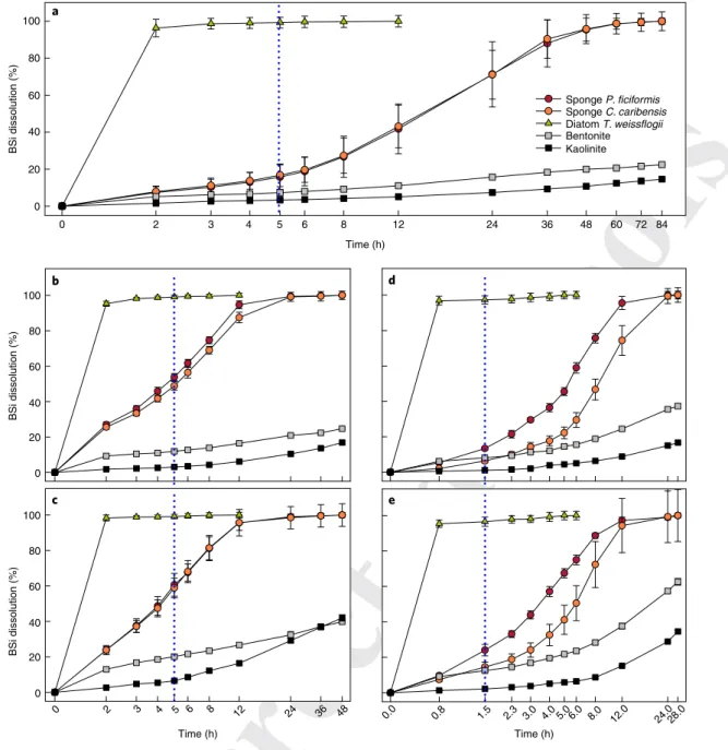
2). The comparative digestion of (1) two types of sponge spicules with different surface area, (2) frustules of cultured diatoms and (3) two forms of lithogenic silica (LSi) represented by kaolinite and benton-ite aluminosilicates (Methods and Supplementary Table 1) revealed major differences in dissolution dynamics. The 1% sodium carbonate approach dissolved 100% of diatom BSi at the recommended diges-tion time (five hours)5,27. In stark contrast, during that digestion time, less than 16.2 ± 6.2% of sponge BSi was dissolved (Fig. 1a), irrespec-tive of obvious specific surface area differences between the sponge spicule types (Fig. 2). Scanning electron microscopy (SEM) after five hours of digestion documented that diatoms BSi were dissolved
completely, whereas this digestion caused only a very incipient dis-solution of the surface of the silica in the two types of assayed spic-ules (Fig. 2). Complete dissolution of the sponge BSi required over 60 hours, whereas most frustules of the assayed diatom had digested entirely after only 2–3 hours (Fig. 1a). To routinely accomplish a 60 hour digestion for sponge BSi is unpractical because a significant amount of the LSi that typically occurs in the sediments will also be dissolved (Fig. 1a), favours an overestimation of BSi contents.
More aggressive alkaline digestions in either sodium carbonate (5% and 22%) or sodium hydroxide (0.2 and 0.5 M) did not improve the sponge BSi detection (Fig. 1b–e): by the time of complete frustule digestion, the sponge skeletons were only dissolved partially, and, by the time of complete digestion of the sponge skeletons, much of the LSi was also dissolved. Indeed, extended or very aggressive diges-tions of marine sediments are systematically avoided in routine BSi
100 80 60 40 20 BSi dissolution (%) 0 100 80 60 40 20 BSi dissolution (%) 0 100 80 60 40 20 BSi dissolution (%) 0 0 2 3 4 5 6 8 12 24 36 48 60 72 84 Time (h) Time (h) Time (h) Sponge P. ficiformis Sponge C. caribensis Diatom T. weissflogii Bentonite Kaolinite 0 2 3 4 5 6 8 12 24 36 48 0.0 0.8 1.5 2.3 3.0 4.0 5.0 6.0 8.0 12.0 24.028.0 a b d c e
Fig. 1 | Digestion kinetics of BSi and LSi pure materials. a–e, Comparative dissolution kinetics of frustules of cultured Thalassiosira weissflogii, needle-like spicules of the sponge Petrosia ficiformis, star-needle-like spicules of the sponge Chondrilla caribensis, bentonite and kaolinite in 1% (ref. 5) (a), 5% (ref. 21)
(b) and 22% (ref. 23) (c) sodium carbonate at 85 °C, as well as in 0.2 M (ref. 25) (d) and 0.5 M (ref. 26) (e) sodium hydroxide at 85 °C. Symbols represent
the average dissolution (%) and error bars are the s.d. values calculated from eight replicates. Time (h) is shown as a logarithmic scale. The blue dotted vertical lines refers to the recommended digestion time for each technique.
A B 130 131 132 133 134 135 136 137 138 139 140 141 142 143 144 145 146 147 148 149 150 151 152 153 154 155 156 157 158 159 160 161 162 163 164 165 166 167 168 169 170 171 172 173 174 175 176 177 178 179 180 181 182 183 184 185 186 187 188 189 190 191 192 193 194 195
Articles
Nature GeoscieNce
determinations to circumvent laborious aluminium (Al)-based cor-rections for LSi contamination21,24,28. Additionally, the particles of sponge BSi that remained after the primary sediment digestion will erroneously be accounted as LSi by any subsequent digestion, which biases the actual Al:Si ratio of aluminosilicates, a parameter, in turn, required to correct the BSi determination24.
The concluding message is that the most widely used method to determine the total BSi in sediments (1% Na2CO3) overlooks more than 80% of the sponge BSi and that the alternative digestion proto-cols also work inefficiently.
Quantifying dark BSi in sediments
The resistance of sponge BSi to digestion in 1% Na2CO3 was sus-pected by DeMaster when he first proposed the method in 19815.
Nevertheless, under the widespread supposition that the contribu-tion of sponges to BSi in marine sediments was ‘insignificant’5,7,29, the importance of overlooking much of the sponge BSi was assumed by the users of the method as an inaccuracy ‘smaller than insignifi-cant‘. Our results here indicate that such a presumption is erroneous. We quantified the relative contribution of diatoms, sponges, radi-olarians and silicoflagellates to total BSi in the 1 cm thick uppermost layer of 17 marine sediment cores. The cores, collected from depths of 3 to 5,204 m, represent an array of depositional environments, which includes continental shelves, slopes, plateaus, seamounts and basin bottoms from different oceans and seas (Supplementary Discussion 1, Supplementary Fig. 1 and Supplementary Table 2).
Light microscopy, digital photography and morphometric soft-ware were used to measure the volume (and then the Si mass) of
4 µm 10 µm 2 µm 20 µm 50 µm 10 µm 10 µm 3 µm 200 µm 3 µm 2 µm 1 µm 30 µm 5 µm 2 µm 2 µm 300 nm b a 1 µm 1 µm 2 µm d c e f g h i j k l n m o p q r s t
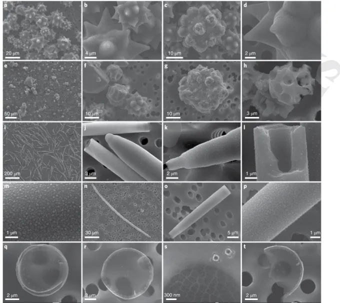
Fig. 2 | Diatom and sponge BSi skeletons during digestion in 1% sodium carbonate at 85 °C. (a–d) The star-like spicules of the sponge C. caribensis after 5 h of digestion show that the bulk of the spicules remain undigested (a) and that only superficial erosion is attained (b and c), which causes tiny pits (c and d). e–h, Spicules of C. caribensis after 48 h of digestion. Most of the stars remain as fragments (e) that can no be longer recognized as spicules, except for few cases (f). Yet a good portion of the initial sponge BSi remains undigested even after 48 h of treatment (g and h). i–m, The needle-like spicules of P.
ficiformis after 5 h of digestion show that most spicules remain undigested (i and j). Increased magnification (k and l) shows that only the silica surface of the spicules is eroded and reveals a granulated pattern that recalls the silica nanospherules (m) formed within the silicification vesicle of the sponge cells during the early silicification steps. n–p, The spicules of P. ficiformis after 48 h of digestion show that fewer recognizable spicules (n) and fragments (o) remain. Again, the progressive digestion of the silica reveals a nanospherule pattern (p). q–t, Frustules of T. weissflogii after 2 h of digestion. Most of the diatoms are entirely dissolved, being no longer detectable. Yet some complete frustules can be found, although their walls are so thin that they become translucent to the electron beam of the SEM, which reveals the porous pattern of the 3 µm pore filter on which the frustules rest (q–t). The delicate ornamentation of the frustules is still visible at high magnification (s).
196 197 198 199 200 201 202 203 204 205 206 207 208 209 210 211 212 213 214 215 216 217 218 219 220 221 222 223 224 225 226 227 228 229 230 231 232 233 234 235 236 237 238 239 240 241 242 243 244 245 246 247 248 249 250 251 252 253 254 255 256 257 258 259 260 261
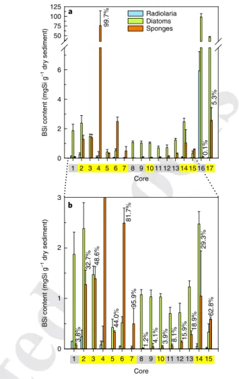
every recognizable sponge spicule, radiolarian and silicoflagellate, either complete or broken. A total of 102,197 spicules, either entire (9.7%) or as fragments (90.3%), as well as 50,183 radiolarians or their fragments and 11,488 silicoflagellates, were processed over five years of microscopy study (Supplementary Fig. 2). The BSi contri-bution of diatoms was estimated from the total BSi content yielded by the 1% sodium carbonate method after discounting the contribu-tion owing to the dissolucontribu-tion (16.2%) of sponge spicules and assum-ing radiolarians as negligible (Methods). The results revealed that the relative contribution of sponge BSi to total BSi was substantial (29.3–99.7%) in 8 of the 17 cores (Fig. 3). These sediments came from continental shelves (cores 3, 5 and 7), slopes (cores 14 and 15) and seamounts (cores 2, 4 and 6). Only one continental shelf envi-ronment—the distal-shelf facies of the Gulf of Cadiz (core 10)—was poor (3.9%) in sponge BSi.
The highest sponge BSi contribution occurred in core 4 (a North Atlantic seamount that hosts sponge aggregations30), in which spic-ules represented over 99% of the total BSi. Sponge BSi also contrib-uted 95.9 and 81.7% in cores 7 and 6 (Fig. 3), respectively, collected from a Mediterranean seagrass meadow and from the base of a sea-mount (Galicia Bank) at the Northeastern Atlantic margin. Spicules were also important (62.8%) at the bathyal slope of the Great Barrier Reef in the Pacific Ocean (core 15). In four other cores (2, 3, 5 and 14) that represent continental slopes and shelves from the North Atlantic and Indian Oceans, sponge BSi was still substantial (29.3–48.6%).
In absolute terms (Fig. 3 and Supplementary Table 3), the largest sponge BSi value (76.31 ± 38.15 mgSi g−1) occurred in core 4 from Flemish Cap, collected within a Geodia spp. ground30, one of the many sponge aggregations that occur over the world’s ocean31. The slope of the Bransfield Strait in Antarctica (core 17), another ocean region in which sponge aggregations abound32–34, ranked second in absolute values of sponge BSi, with 2.57 ± 0.86 mgSi g−1. However, in this Antarctic sediment, sponge spicules represented only 5.3% of the total BSi, which was dominated by diatoms (45.69 ± 2.32 mgSi g−1). Frustules were even more abundant (98.56 ± 8.53 mgSi g−1) in core 16, from a Southern Ocean siliceous-ooze area35, in which sponge spicules were very rare (0.13%). In summary, in most sediments from relatively open-water environments, such as the Girona conti-nental rise (core 8), central basins (cores 9, 11–13 and 16) and slope basins (core 1), the sponge BSi contribution was comparatively small (<25%).
Silicifiers other than diatoms and sponges always contributed marginally. Siliceous radiolarians were regularly detected in ten cores (1, 2, 4–6, 10 and 14–17), but did not represent much of the total BSi (Fig. 3 and Supplementary Table 3). Radiolarian BSi reached its maximum (5.94 ± 1.30 mgSi g−1) in the Southern Ocean biosiliceous ooze (core 16), in agreement with previous knowledge that reported patches of abundant radiolarian skeletons scattered across this and other ocean areas35–37. Nevertheless, that Southern Ocean BSi-rich (104.80 mgSi g−1) sediment was dominated by frus-tules (94.1%), with radiolarians contributing only 5.7% of the total BSi. Silicoflagellates were even less important globally, not being retrieved in the uppermost sediments of most cores. Their best representation occurred in Southern Ocean cores, although their maximum contribution (0.17% in core 16) was still insignificant (Supplementary Table 3).
These results indicate that, unlike traditionally hypothesized, a significant portion of the BSi at the superficial sediment layer of continental margins and around seamounts comes from sponges, and not only from diatoms (Supplementary Discussion 2).
Preservation of dark BSi
The low solubility of sponge BSi has enabled such a Si reservoir to pass unnoticed in routine digestions to quantify the total BSi in marine sediments. The question arises now as to whether the
omis-sion may have led to a substantial underestimate of the Si burial in the global oceans.
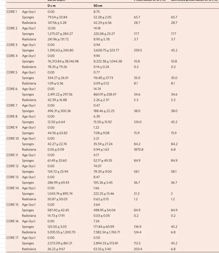
In practical terms, the BSi deposited at the sediments continues to dissolve during its burial until a saturating silicate concentra-tion is reached in the interstitial water. This typically happens no deeper than 30–35 cm in the sediments8,21,38. To be conservative, we regarded that BSi preservation starts not at a 30 cm burial depth but at 50 cm. The sponge BSi preservation was then quantified in each core as the difference (%) in sponge BSi content between the 1 cm thick upper sediment layer and that buried at 50 cm, after assuming an approximately constant rate of sponge BSi deposition (Methods). In our cores, sponge BSi preservation ranged from 10.8 to 84.9% (Table 1). Overrated preservation (>100%) resulted in four cores: the Bay of Brest (core 3), the turbiditic Girona rise (core 8), the Southern Ocean biosiliceous oozes (core 16) and the Antarctic slope (core 17), and these were not considered when calculating the average BSi preservation (Supplementary Discussion 3). Not to overestimate in subsequent calculations, it was assumed that the
125 100 75 50 6 4 2 0 Radiolaria Diatoms Sponges 99.7% 0.1% 5.3%
BSi content (mgSi g
–1 dr
y sediment)
BSi content (mgSi g
–1 dr y sediment) 2 3 1 0 32.7% 48.6% 3.8% 44.0% 95.9% 1.2% 4.1% 3.9% 8.1% 15.9% 18.9% 62.8% 29.3% 81.7% 1 2 3 4 5 6 7 8 9 10 11 12 13 14 15 1 2 3 4 5 6 7 8 9 10 Core Core 11 12 13 14 15 16 17 a b
Fig. 3 | Contributors of BSi in superficial sediments. a, Mean (±s.d.) content of BSi from diatoms, sponges and radiolarians in the 1 cm thick uppermost layer of sediment of each of the 17 studied cores. b, The graph with BSi contents lower than 3 mgSi g−1 (except core 4) makes visible the minor contributions of some BSi types into some cores. Percentages above the orange bars indicate the relative contribution of sponge BSi to total BSi in the sediments (absolute values are given in Supplementary Table 3). The sponge BSi contribution was substantial (29–99%) in cores from continental margins and around seamounts (core numbers with a yellow background). Diatom BSi dominated the remaining cores, mostly collected below open waters in ocean basins (core numbers with a grey background).
A B 262 263 264 265 266 267 268 269 270 271 272 273 274 275 276 277 278 279 280 281 282 283 284 285 286 287 288 289 290 291 292 293 294 295 296 297 298 299 300 301 302 303 304 305 306 307 308 309 310 311 312 313 314 315 316 317 318 319 320 321 322 323 324 325 326 327
Articles
Nature GeoscieNce
preservation in each of the overrated cores could not be higher than the average value that resulted from the 13 remaining ones (Table 1). Such a ‘correction’ is conservative because an averaged preservation
is applied to sediments of the Southern Ocean (cores 16 and 17) and the Bay of Brest (core 3), which are
known to be characterized by a greater preservation than the average in marine sediments39,40.
Q6
Table 1 | Preservation (%) of sponge and radiolarian BSi
Burial depth Preservation of Si (%) Corrected preservation of Si (%)
0 c m 50 cm
CORE 1 Age (kyr) 0.00 8.75
Sponges 79.54 ± 33.84 52.28 ± 2.05 65.7 65.7
Radiolaria 147.56 ± 5.28 42.29 ± 6.56 28.7 28.7
CORE 2 Age (kyr) 12.00 14.18
Sponges 1,275.07 ± 284.27 225.08 ± 23.27 17.7 17.7
Radiolaria 241.96 ± 131.72 8.90 ± 5.78 3.7 3.7
CORE 3 Age (kyr) 0.00 0.94
Sponges 1,390.63 ± 240.80 3,608.75 ± 323.77 259.5 45.2
CORE 4 Age (kyr) 0.00 9.94
Sponges 76,313.84 ± 38,146.98 8,222.38 ± 1,044.38 10.8 10.8
Radiolaria 78.35 ± 79.26 0.14 ± 0.24 0.2 0.2
CORE 5 Age (kyr) 0.00 0.77
Sponges 334.27 ± 26.01 116.85 ± 37.73 35.0 35.0
Radiolaria 1.09 ± 0.36 0.09 ± 0.12 8.1 8.1
CORE 6 Age (kyr) 0.00 14.74
Sponges 2,491.22 ± 297.36 860.91 ± 258.47 34.6 34.6
Radiolaria 42.39 ± 16.88 2.26 ± 2.37 5.3 5.3
CORE 7 Age (kyr) 0.00 0.47
Sponges 496.31 ± 300.36 188.46 ± 22.25 38.0 38.0
CORE 8 Age (kyr) 0.00 6.39
Sponges 12.50 ± 6.64 15.50 ± 15.92 124.0 45.2
CORE 9 Age (kyr) 0.00 1.22
Sponges 44.56 ± 63.82 7.08 ± 9.08 15.9 15.9
CORE 10 Age (kyr) 0.00 2.21
Sponges 42.27 ± 22.74 35.59 ± 27.24 84.2 84.2
Radiolaria 0.05 ± 0.09 0.94 ± 1.63 1870.8 6.8
CORE 11 Age (kyr) 0.00 4.17
Sponges 61.49 ± 33.60 52.17 ± 49.35 84.9 84.9
CORE 12 Age (kyr) 0.00 74.07
Sponges 134.72 ± 25.94 78.30 ± 9.00 58.1 58.1
CORE 13 Age (kyr) 0.00 8.47
Sponges 286.99 ± 69.43 105.36 ± 5.45 36.7 36.7
CORE 14 Age (kyr) 0.00 1.66
Sponges 1,043.74 ± 895.74 222.25 ± 13.46 21.3 2
Radiolaria 50.87 ± 50.03 0.62 ± 0.15 1.2 1.2
CORE 15 Age (kyr) 0.00 3.64
Sponges 587.40 ± 42.45 498.95 ± 54.04 84.9 84.9
Radiolaria 14.73 ± 17.91 0.03 ± 0.05 0.2 0.2
CORE 16 Age (kyr) 0.00 7.24
Sponges 125.50 ± 3.03 171.84 ± 60.99 136.9 45.2
Radiolaria 5,935.55 ± 1,300.70 7,382.34 ± 1,765.71 124.4 6.8
CORE 17 Age (kyr) 0.00 0.50
Sponges 2,572.09 ± 861.21 2,894.33 ± 513.81 112.5 45.2
Radiolaria 26.22 ± 9.67 53.33 ± 3.40 203.4 6.8
Estimated from the difference in BSi content (µgSi g–1 sed) between the superficial sediment and that buried at 50 cm. Sediment age at 50 cm is given. Overrated preservation (>100%) resulted in
some cores (Supplementary Discussion 3), which were not considered when calculating average preservation (%) for sponge and radiolarian BSi. Subsequent calculations that involved overrated cores conservatively assumed a ‘corrected preservation’ identical to the average that resulted from the pool of the remaining cores.
328 329 330 331 332 333 334 335 336 337 338 339 340 341 342 343 344 345 346 347 348 349 350 351 352 353 354 355 356 357 358 359 360 361 362 363 364 365 366 367 368 369 370 371 372 373 374 375 376 377 378 379 380 381 382 383 384 385 386 387 388 389 390 391 392 393
Calculations yielded a global average preservation of 45.2 ± 27.4% for sponge BSi and 6.8 ± 10.1% for radiolarian BSi. Diatom BSi pres-ervation, estimated from the literature8, is 8%. The comparison of these three values indicates that sponge BSi has a great potential for Si burial (Supplementary Figs. 2 and 3).
Burial flux of dark BSi
The
global burial flux of sponge and radiolarian BSi is quanti-fied herein. Ocean extension was calculated41 at 361.88 × 10⁶ km2 (Methods). As we noticed marked differences between ‘basin environments’ and ‘continental-margin–seamount environments’ regarding sponge BSi content in sediments, the ocean was simpli-fied to those main compartments, where basins represent 70.2% of the seafloor. The remaining 29.8% consists of an assemblage of continental margins plus seamounts, plateaus and other minor geo-morphological features. The continental-margin–seamount com-partment is represented by ten cores and the basin comcom-partment by seven (Fig. 3, Supplementary Discussion 1 and Supplementary Table 2). We then estimated the age of the sediments at 50 cm, wet bulk density of the sediments and the amount of sponge BSi preserved at 50 cm (Table 2 and Methods). By combining all four of these parameters, the amount of sponge BSi buried per metre squared and year was finally calculated for each core (Table 2). The mean rates of sponge BSi burial spanned two orders of magnitude across cores of the continental-margin–seamount compartment, from 13.3 mgSi m−2 yr−1 at the deep continental shelf of the Gulf of Cadiz (core 10) to 1,877.7 mgSi m−2 yr−1 at the Antarctic slope (core 17). The span illustrates the large sampled variety of depositional environments (Supplementary Discussion 3). In the basin compart-ment, sponge BSi preservation reflects the relatively homogeneous depositional scenario expected for distal-margin and open-water environments, with low rates varying minimally across five of the seven cores (4.5–9.9 mgSi m−2 yr−1). The preservation of sponge BSi was even lower at the Western Mediterranean continental rise (core 8) and the Pacific Clarion–Clipperton fracture zone (core 12) ((0.7 and 0.8 mgSi m−2 yr−1), respectively). Unlike that known for
plank-Q7
tonic diatoms, the burial rate of sponge BSi barely correlates with the sediment deposition rate (Supplementary Fig. 4a). The non-plank-tonic nature of the sponge BSi production disrupts the relationship (Supplementary Discussion 3). Neither did sponge BSi preserva-tion (%) correlate with total BSi in the sediments (Supplementary Fig. 4b), because of the general resistance of spicules to dissolution (Supplementary Discussion 3).
The approach used for sponge BSi was also extended to radiolar-ian BSi. Siliceous radiolarradiolar-ians occurred in only 10 of the 17 cores, with estimated burial rates from 0.1 × 10⁻² to 38.7 mgSi m−2 yr−1, and preservation percentages varying from 0.2 to 28.7% (Tables 1 and
2). As in the case of sponge BSi, overrated radiolarian preserva-tion in the Southern Ocean sediments (cores 16 and 17) had to be adjusted down to the global average (6.8 ± 10.1%), as well as in core 10 (Supplementary Discussion 3).
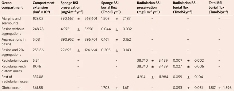
The global burial flux for the sponge and radiolarian BSi in the ocean was then estimated by multiplying the preservation rates across the extension of the pertinent ocean compartments for each organism type (Table 3). For sponge BSi, the extensions of the conti-nental-margin–seamount and basin compartments were calculated and the mean BSi burial rate that resulted from the corresponding set of associated cores applied (Methods). Yet, sponge aggregations occur in basins of all oceans31, but their potential BSi contribution was not incorporated in the set of ‘basin cores’ because samples of abyssal sponge grounds are lacking in the repositories. Evidence from both the literature33,42,43 and cores 4, 5 and 17, which represent aggregations on continental margins, suggests that the sponge BSi content in the sediments of aggregations may be orders of magni-tude higher than those in sponge-lacking areas. To address the lack of representability of sponge grounds in basin cores, we assumed that about 2% of the seafloor in basins hosts sponge aggregations. Such an assumption is thought to be conservative. Observations and predictive modelling on the occurrence of sponge grounds between 200 and 5,000 m in the North Atlantic—the best-studied ocean area in this regard—suggest a global occupancy much larger than 2%, with sponge grounds that extend over 33.5% of the Exclusive
Table 2 | Age, wet bulk density and deposition rate of the sediment in the different cores
Core Age at 50 cm (yr) Sediment density (g cm–3) Deposition rate (g sed m–2 yr−1) Sponge BSi at 50 cm (µgSi g–1) Sponge BSi burial rate (mgSi m−2 yr−1) Radiolarian BSi at 50 cm (µgSi g−1) Radiolarian BSi burial rate (mgSi m−2 yr−1) 1 8,754 1.557 88.915 52.277 4.648 42.285 3.760 2 2,182 1.601 366.824 225.082 82.566 8.901 3.265 3 944 1.659 879.051 628.600 552.571 – – 4 9,937 1.618 81.396 8,222.379 669.271 0.137 0.011 5 767 1.652 1,077.287 116.852 125.883 0.089 0.095 6 14,741 1.552 52.641 860.915 45.319 2.263 0.119 7 471 1.660 1,763.031 188.459 332.260 – – 8 6,390 1.563 122.309 5.649 0.691 – – 9 1,217 1.554 638.807 7.079 4.522 – – 10 2,212 1.654 373.797 35.587 13.302 0.003 0.001 11 4,170 1.586 190.157 52.172 9.921 – – 12 74,074 1.441 9.728 78.295 0.762 – – 13 8,475 1.418 83.680 105.364 8.817 – – 14 1,661 1.464 440.747 222.253 97.957 0.616 0.272 15 3,643 1.604 220.143 498.947 109.840 0.032 0.007 16 7,236 1.395 96.365 56.728 5.467 402.017 38.740 17 500 1.615 1,615.018 1,162.650 1,877.701 1.776 2.868
The amount of BSi preserved at 50 cm burial depth (considering corrected BSi preservation for sponges in cores 3, 8, 16 and 17 and for radiolarians in cores 10, 16 and 17) and the derived BSi burial rates for sponges and radiolarians. The continental-margin–seamounts compartment is represented by cores 2–7, 10, 14, 15 and 17. The basin compartment is represented by cores 1, 8, 9, 11–13 and 16.
A B 394 395 396 397 398 399 400 401 402 403 404 405 406 407 408 409 410 411 412 413 414 415 416 417 418 419 420 421 422 423 424 425 426 427 428 429 430 431 432 433 434 435 436 437 438 439 440 441 442 443 444 445 446 447 448 449 450 451 452 453 454 455 456 457 458 459
Articles
Nature GeoscieNce
Economic Zone and High Seas in Greenland, 25.5% in Norway, 14.8% in Iceland, 10.5% in the Faeroes, 5.6% in Canada and so on44. Therefore, to consider the effects of sponge aggregations in basins (Table 3), we applied the average burial rate (890.9 ± 896.7 mg S m2 yr−1) that results from the three cores that involve sponge aggre-gations (cores 4, 5 and 17). The final calculations yielded a global burial flux through sponge BSi of 1.7 ± 1.6 TmolSi yr−1 (Table 3). Note that error propagation incorporating the marked differences in the BSi burial rate across cores from very different environments in the world’s oceans leads to a large s.d. value.
We
applied the same reasoning to radiolarian BSi, but considered the ocean compartments for these planktonic organisms to be dif-ferent from those defined for sponges (Table 3). A recent mapping of the seafloor sediments36 identified many small areas across the ocean seafloor characterized by the abundance of radiolarian skel-etons in the sediments (oozes). By importing into ArcGis Software the available map layers, we determined that radiolarian oozes con-sist of a total of 64 patches with a global extension of 5.3 × 10⁶ km2 and that radiolarian-rich diatom oozes occupied 19.5 × 10⁶ km2, mostly in the Southern Ocean (Supplementary Fig. 5). To those extensions, the BSi content and preservation values of core 16, which testified for radiolarian abundance in the oozes (Fig. 3), were applied (Table 3). For the rest of the ocean, the average that results from all cores, core 16 included, was used. This was done to incor-porate the notion that additional patches of radiolarian oozes occur, though not yet identified36. The global calculations yielded a burial flux through radiolarian BSi of 9.3 ± 5.1 × 10⁻² TmolSi yr−1, that is, two orders of magnitude lower than that of sponge BSi. Yet, these calculations for radiolarian BSi must be seen as a first conservative attempt to set the global magnitude of the burial flux. Subsequent readjustments based on the empirical determination of local pres-ervation values may be required to relax our very conservative sce-nario that radiolarian BSi preservation in the oozes is only 6.8% (Supplementary Discussion 3 and Supplementary Table 4).
Collectively, the burial of dark BSi, quantified herein through sponge and radiolarian skeletons, increases by 28.6% the previous value of the biological Si sink (6.3 ± 3.6 TmolSi yr−1), which consid-ered only diatoms. Sponge BSi accounts for 94.8% of that increase, with a minor (5.2%) global contribution from radiolarians. The identified Si sink through dark BSi (−1.8 ± 1.4 TmolSi yr−1) rises
Q8
the global output flux to 12.8 TmolSi yr−1 and brings the ocean bud-get close to equilibrium, but now with a subtle negative imbalance (−0.7 TmolSi yr−1). Such a small gap is likely to be filled readily, because recent studies have reported small, local Si inputs into the ocean through DSi-rich ground water10,45–47, which await quantifica-tion.
online content
Any methods, additional references, Nature Research reporting summaries, source data, statements of code and data availability and associated accession codes are available at https://doi.org/10.1038/ s41561-019-0430-7.
Received: 2 February 2018; Accepted: 17 July 2019; Published: xx xx xxxx
References
1. Nelson, D. M., Tréguer, P., Brzezinski, M. A., Leynaert, A. & Quéguiner, B. Production and dissolution of biogenic silica in the ocean: revised global estimates, comparison with regional data and relationship to biogenic sedimentation. Glob. Biogeochem. Cycles 9, 359–372 (1995).
2. Tréguer, P. & Pondaven, P. Silica control of carbon dioxide. Nature 406, 358–359 (2000).
3. Harriss, R. C. Biological buffering of oceanic silica. Nature 212, 275–276 (1966).
4. Calvert, S. E. Silica balance in the ocean and diagenesis. Nature 219, 919–920 (1968).
5. DeMaster, D. J. The supply and accumulation of silica in the marine environment. Geochim. Cosmochim. Acta 45, 1715–1732 (1981).
6. Tréguer, P. et al. The silica balance in the world ocean: a reestimate. Science 268, 375–379 (1995).
7. Laruelle, G. G. et al. Anthropogenic perturbations of the silicon cycle at the global scale: key role of the land-ocean transition. Glob. Biogeochem. Cycles 23, GB4031 (2009).
8. Tréguer, P. J., De La & Rocha, C. L. The world ocean silica cycle. Ann. Rev.
Mar. Sci. 5, 477–501 (2013).
9. Frings, P. J., Clymans, W., Fontorbe, G., De La Rocha, C. & Conley, D. J. The continental Si cycle and its impact on the ocean Si isotope budget. Chem.
Geol. 425, 12–36 (2017).
10. Hawkings, J. R. et al. Ice sheets as a missing source of silica to the polar oceans. Nat. Commun. 8, 14198 (2017).
11. Rahman, S., Aller, R. C. & Cochran, J. K. The missing silica sink: revisiting the marine sedimentary Si cycle using cosmogenic 32Si. Glob. Biogeochem.
Cycles 31, 1559–1578 (2017).
Table 3 | Preservation rates and burial fluxes for dark BSi through sponges and radiolarian skeletons in their ocean compartments
ocean
compartment Compartmentextension (km2 × 106) Sponge BSi preservation (mgSi m−2 yr−1) Sponge BSi burial flux (tmolSi yr−1) Radiolarian BSi preservation (mgSi m−2 yr−1) Radiolarian BSi burial flux (tmolSi yr−1) total BSi burial flux (tmolSi yr−1) Margins and seamounts 108.02 390.667 ± 568.601 1.503 ± 2.187 – – – Basins without aggregations 248.78 4.975 ± 3.556 0.044 ± 0.032 – – – Aggregations in basins 5.08 890.952 ± 896.701 0.161 ± 0.162 – – – Basins and 2% aggregations 253.86 22.695 ± 124.664 0.205 ± 0.143 – – – Radiolarian oozes 5.34 – – 38.740 ± 8.489 0.007 ± 0.002 – Radiolarian-rich diatom oozes 19.46 – – 38.740 ± 8.489 0.027 ± 0.006 – Rest of ‘radiolarian’ ocean 337.08 – – 4.914 ± 11.984 0.059 ± 0.104 – Global ocean 361.88 – 1.708 ± 1.611 – 0.093 ± 0.051 1.801 ± 1.396
For sponges, the ocean seafloor was divided into two compartments, ‘continental margins, seamounts and minor additional geomorphological features’ versus ‘ocean basins’, with about 2% of abyssal (or deeper) basin bottoms estimated to contain sponge aggregations. For radiolarians, the ocean floor was divided into three major compartments: radiolarian oozes, radiolarian-rich diatom oozes (that is, sediment dominated by diatom frustules but still rich in siliceous radiolarian testa) and the rest of the ocean (Supplementary Fig. 5).
460 461 462 463 464 465 466 467 468 469 470 471 472 473 474 475 476 477 478 479 480 481 482 483 484 485 486 487 488 489 490 491 492 493 494 495 496 497 498 499 500 501 502 503 504 505 506 507 508 509 510 511 512 513 514 515 516 517 518 519 520 521 522 523 524 525
12. Rahman, S., Tamborski, J. J., Charette, M. A. & Cochran, J. K. Dissolved silica in the subterranean estuary and the impact of submarine groundwater discharge on the global marine silica budget. Mar. Chem. 208, 29–42 (2019). 13. Tréguer, P. J. The Southern Ocean silica cycle. C. R. Geosci. 346, 279–286
(2014).
14. Maldonado, M. et al. Siliceous sponges as a silicon sink: an overlooked aspect of the benthopelagic coupling in the marine silicon cycle. Limnol. Oceanogr. 50, 799–809 (2005).
15. Maldonado, M., Navarro, L., Grasa, A., Gonzalez, A. & Vaquerizo, I. Silicon uptake by sponges: a twist to understanding nutrient cycling on continental margins. Sci. Rep. 1, 30 (2011).
16. Maldonado, M., Riesgo, A., Bucci, A. & Rützler, K. Revisiting silicon budgets at a tropical continental shelf: silica standing stocks in sponges surpass those in diatoms. Limnol. Oceanogr. 55, 2001–2010 (2010).
17. Maldonado, M., Ribes, M. & Van Duyl, F. C. Nutrient fluxes through sponges: biology, budgets, and ecological implications. Adv. Mar. Biol. 62, 114–182 (2012).
18. Chu, J. W. F., Maldonado, M., Yahel, G. & Leys, S. P. Glass sponge reefs as a silicon sink. Mar. Ecol. Prog. Ser. 441, 1–14 (2011).
19. Jochum, K. P. et al. Whole-ocean changes in silica and Ge/Si ratios during the Last Deglacial deduced from long-lived giant glass sponges. Geophys. Res.
Lett. 44, 11,555–511,564 (2017).
20. Jochum, K. P., Wang, X., Vennemann, T. W., Sinha, B. & Müller, W. E. G. Siliceous deep-sea sponge Monorhaphis chuni: a potential paleoclimate archive in ancient animals. Chem. Geol. 300–301, 143–151 (2012). 21. Hurd, D. C. Interactions of biogenic opal, sediment and seawater in the
Central Equatorial Pacific. Geochim. Cosmochim. Acta 37, 2257–2282 (1973). 22. Mortlock, R. A. & Froelich, P. N. A simple method for the rapid
determination of biogenic opal in pelagic marine sediments. Deep -Sea Res. I 36, 1415–1426 (1989).
23. Eggimann, D. W., Manheim, F. T. & Betzer, P. R. Dissolution and analysis of amorphous silica in marine sediments. J. Sediment Petrol. 50, 215–225 (1980).
24. Kamatani, A. & Oku, O. Measuring biogenic silica in marine sediments. Mar.
Chem. 68, 219–229 (2000).
25. Paasche, E. Silicon and the ecology of marine plankton diatoms. II Silicate-uptake kinetics in five diatom species. Mar. Biol. 19, 262–269 (1973).
26. Müller, P. J. & Schneider, R. An automated leaching method for the determination of opal in sediments and particulate matter. Deep-Sea Res I 40, 425–444 (1993).
27. Conley, D. J. An interlaboratory comparison for the measurements of biogenic silica in sediments. Mar. Chem. 63, 39–48 (1998).
28. Ragueneau, O. et al. A new method for the measurement of biogenic silica in suspended matter of coastal waters: using Si:Al ratios to correct for the mineral interference. Cont. Shelf Res 25, 697–710 (2005).
29. Heinze C. in The Silicon Cycle: Human Perturbations and Impacts on Aquatic
Systems (eds Ittekkot, V., Unger, D., Humborg, C. & An, N. T.) 229–244
(SCOPE Series Vol. 66, Island Press, 2006).
30. Murillo, F. J., Kenchington, E., Lawson, J. M., Li, G. & Piper, D. J. W. Ancient deep-sea sponge grounds on the Flemish Cap and Grand Bank, northwest Atlantic. Mar. Biol. 163, 1–11 (2016).
31. Maldonado M., et al. in Marine Animal Forests: The Ecology of Benthic
Biodiversity Hotspots (eds Rossi, S., Bramanti, L., Gori, A. Orejas C.) 145–183
(Springer International, 2017).
32. Dayton, P. K. Observations of growth, dispersal and population dynamics of some sponges in McMurdo Sound, Antarctica. Colloq. Int. Cent. Natl Rech.
Sci. 291, 271–282 (1979).
33. Gutt, J., Böhmer, A. & Dimmler, W. Antarctic sponge spicule mats shape macrobenthic diversity and act as a silicon trap. Mar. Ecol. Prog. Ser. 480, 57–71 (2013).
34. Barthel, D. & Gutt, J. Sponge associations in the eastern Weddell Sea. Antarct.
Sci. 4, 137–150 (1992).
35. Lisitzin A. P. in The Micropaleontology of Oceans (eds Funnell, B. M. & Riedel W. R.) 173–195 (Cambridge Univ. Press, 1971).
36. Dutkiewicz, A., Müller, R. D., O’Callaghan, S. & Jónasson, H. Census of seafloor sediments in the world’s ocean. Geology 43, 795–798 (2016).
37. Boltovskoy, D., Kling, S. A., Takahashi, K. & Bjørklund, K. World atlas of distribution of recent Polycystina (Radiolaria). Palaeontol. Electron. 13, 1–230 (2010).
38. Van Cappellen, P. & Qiu, L. Biogenic silica dissolution in sediments of the Southern Ocean. I. Solubility. Deep-Sea Res II 44, 1109–1128 (1997). 39. DeMaster, D. J. The accumulation and cycling of biogenic silica in the
Southern Ocean: revisiting the marine silica budget. Deep-Sea Res II 49, 3155–3167 (2002).
40. Ragueneau, O. et al. Biodeposition by an invasive suspension feeder impacts the biogeochemical cycle of Si in a coastal ecosystem (Bay of Brest, France).
Biogeochemistry 75, 19–41 (2005).
41. Harris, P. T., Macmillan-Lawler, M., Rupp, J. & Baker, E. K. Geomorphology of the oceans. Mar. Geol. 352, 4–24 (2014).
42. Bett, B. J. & Rice, A. L. The influence of hexactinellid sponge spicules on the patchy distribution of macrobenthos in the Porcupine Seabight (bathyal NE Atlantic). Ophelia 36, 217–226 (1992).
43. Laguionie-Marchais, C., Kuhnz, L. A., Huffard, C. L., Ruhl, H. A. & Smith, K. L. Jr Spatial and temporal variation in sponge spicule patches at Station M, northeast Pacific. Mar. Biol. 162, 617–624 (2015).
44. Howell, K.-L., Piechaud, N., Downie, A.-L. & Kenny, A. The distribution of deep-sea sponge aggregations in the North Atlantic and implications for their effective spatial management. Deep-Sea Res I 115, 309–320 (2016).
45. Sospedra, J. et al. Identifying the main sources of silicate in coastal waters of the Southern Gulf of Valencia (Western Mediterranean Sea). Oceanologia 60, 52–64 (2018).
46. Ehlert, C. et al. Transformation of silicon in a sandy beach ecosystem: insights from stable silicon isotopes from fresh and saline groundwaters.
Chem. Geol. 440, 207–218 (2016).
47. Lecher, A. Groundwater discharge in the Arctic: a review of studies and implications for biogeochemistry. Hydrology 4, 41 (2017).
Acknowledgements
We thank the British Ocean Sediment Core Research Facility (BOSCORF-NOC) for providing access to cores 1, 12, 14 and 16. We also thank E. Kenchington, C. Campbell, K. Jarrett and J. Murillo (BIO) for making the data and sediment of cores 2 and 4 available. A. Ehrhold (IFREMER) is thanked for core 3, M. A. Mateo (CEAB) for core 7 and T. Whiteway (Australian Geosciences) for core 15. R. Ventosa and M. Abad are thanked for helping with the DSi autoanalyser determinations, B. Dursunkaya for helping with the digestion experiments and P. Talberg and L. Cross for providing strains of the
Thalassiossira diatom. J. Krause is especially thanked for comments and insight on the
manuscript. This study, which spanned five years, benefitted from funding by two grants of the Spanish MINECO (CTM2012-37787 and CTM2015-67221-R). Financial support by the European Union’s Horizon 2020 research and innovation program to the SponGES project (grant agreement 679849) is acknowledged.
Author contributions
M.M. designed the study and experiments. Sediment and BSi digestions were conducted by M.M., M.L.A., C.S., M.G.-P. and C.G. Light microscopy determination of the BSi was conducted by M.L.A., C.S., M.G.-P. and C.G. under supervision by M.M. SEM and energy dispersive X-ray spectrometry analyses were conducted by M.M. and C.S. Data analyses were conducted by M.M. and M.L.A. and ArcGis mapping by M.G.-P. M.M. wrote the manuscript, with invaluable inputs made by M.L.A. and the rest of co-authors at different stages of the process.
Competing interests
The authors declare no competing interests.
Additional information
Supplementary information is available for this paper at https://doi.org/10.1038/ s41561-019-0430-7.
Reprints and permissions information is available at www.nature.com/reprints.
Correspondence and requests for materials should be addressed to M.M.
Publisher’s note: Springer Nature remains neutral with regard to jurisdictional claims in
published maps and institutional affiliations.
A B 526 527 528 529 530 531 532 533 534 535 536 537 538 539 540 541 542 543 544 545 546 547 548 549 550 551 552 553 554 555 556 557 558 559 560 561 562 563 564 565 566 567 568 569 570 571 572 573 574 575 576 577 578 579 580 581 582 583 584 585 586 587 588 589 590 591
Articles
Nature GeoscieNce
Methods
Digestion of silica. Dissolution kinetics of several forms of BSi and LSi were compared using different digesters. As BSi, we used nitric-acid-cleaned frustules of T. weissflogii (cultured using F2 media), needle-like (oxea) spicules of P.
ficiformis and star-like spicules (cortical spherasters) of C. caribensis. As LSi, we
used aluminosilicate bentonite (Sigma-Aldrich, Pcode 101190698, H2Al2O6Si) and
kaolinite (Fluka, Pcode 100981947, Al2O3·2SiO2·2H2O). Varying dry weights for
the different materials were used in the digestions (Supplementary Table 1), so that the total amount of Si to be released during the digestion was similar across the materials (1.25 ± 0.09 mgSi). To make sure that the resulting DSi concentrations always remained far below the saturating concentration, we increased the volume of digester from 10 ml (traditional approach) to 40 ml, which provided solvent in great excess. All the digestions were based on eight replicated subsamples of each material. The assayed digestion solutions were sodium carbonate at 1% (ref. 5), 5% (ref. 21) and
22% (ref. 23), as well as sodium hydroxide at 0.2 M (ref. 25) and 0.5 M (ref. 26).
Digestions were conducted in 50 ml hermetically closed Teflon bombs immersed in distilled water at 85 °C with orbital agitation, using a 50 l SBS TBA-30 bath that was user modified for agitation and temperature control. Sodium carbonate digestions at 1, 5 and 22% were sampled at 0, 2, 3, 4, 5, 6, 8, 12, 24, 48, 60, 72 and 84 h. The more aggressive sodium hydroxide digestions (0.2 and 0.5 M) were sampled at 0, 0.75, 1.5, 2.25, 3, 4, 5, 6, 8, 12, 24, and 28 h. For each sample, 1 ml of the digestion solution was pipetted out after centrifugation of the Teflon bombs at 1,500 rpm for 3 min. The sampled digestion solution was added to 19 ml of HCl solution for buffering and termination of the digestion reaction, with the pH of the resulting mix brought down to 6, an optimal value for the colorimetric determination of Si concentration (±1%) using an Alliance Futura autoanalyser. Finally, the percentage of Si released during the digestions was plotted against time to depict between-material differences in the dissolution kinetics. Additionally, two spare Teflon tubes of each material were poured on a 0.45 cm polycarbonate filter (3 µm pore) at each sampling time. The retained particulate BSi material was subsequently inspected under a Hitachi TM3000 SEM equipped with an energy dispersive X-ray spectrometer for microanalysis, and subsequently carbon coated and examined under a high-resolution Jeol Field Emission J1700S SEM.
To digest sediment from the cores, we used sodium carbonate at 1%, following DeMaster’s technique27,48. The method assumes that most of the BSi is dissolved in
about 3 h at 85 °C and that the additional Si leached from the LSi can be corrected using the intercept of the linear regression to depict the increase in DSi caused by the progressive LSi digestion during 3, 4 and 5 h. Analyses were based on five sediment subsamples of 30 mg each.
Sediment cores. The investigated cores (Supplementary Table 2) represent a diverse array of sedimentary marine environments (Supplementary Discussion 1). Cores 1 (Challenger, Dec-58, 51719_13; Porcupine Seabigth, Northeastern Atlantic), 12 (James Cook 120–081, GC-05; Northeastern Pacific basin), 14 (Sonne SO200, SO200/15PC; Sumatra margin, Indian Ocean) and 16 (James Clark Ross, JR179, PC501; Southern Ocean) were provided by the British Ocean Sediment Core Research Facility (of the National Oceanography Centre. Cores 2 (Hudson 20110310062-pc; Flemish Cap plateau, Northwestern Atlantic) and 4 (2009061 0058 A; Flemish Cap seamount, Northwestern Atlantic) were provided by the Geological Survey of Canada, Marine Geoscience Collection Facility at the Bedford Institute of Oceanography. Core 3 (SRQ3-KS34; Bay of Brest, Northeastern Atlantic) was supplied by the Marine Geoscience research unit at IFREMER. Core 5 (MLB2017-001-006; Sambro Bank, Northwestern Atlantic) was a push core sampled in September 2017 by using ROPOS ROV on the Nova Scotia shelf during the SponGES H2020 project. Cores 6 (K11-ERGAP2; Galicia Bank, Northeastern Atlantic), 8 (TG 36, GC-88-1; Mediterranean Iberian margin), 9 (KF14, VALSIS; Valencia Trough, Western Mediterranean), 10 (TG51bis, GC86-2; Gulf of Cadiz, North Eastern Atlantic), 11 (ALM6, MAYC-96; Alboran Basin, Western Mediterranean), 13 (TG3, ORINOCO97; Guiana Basin, Northwestern Atlantic) and 17 (TG15, MAGIA-99; Bransfield Strait, Antarctica) were provided by the Marine Geosciences department at the Institute of Marine Sciences (ICM, CSIC). Core 7 (C-2000; Mediterranean Iberian Margin) was provided by the Macrophyte Ecology Group at the Center for Advanced Studies of Blanes (CEAB, CSIC). Core 15 (NEA 3, 1987, 75/GC05; Great Barrier Reef, Queensland Trough) was provided by Australian Geosciences. Coring was based on gravity (cores 1, 3, 8, 10, 11, 12, 13, 15 and 17), piston (cores 2, 6, 7, 9, 14 and 16), box-core (core 4) or push-core (push-core 5) methodologies. All the sediments were dried to a constant weight before digestion and microscopy analyses.
Determination of dark BSi. For the microscope determination of sponge, radiolarian and silicoflagellate BSi in sediments (mgSi per gram of dry sediment), three dry sediment subsamples of 10 mg each were collected and transferred to test tubes, boiled in HCl to remove calcareous skeletons, then in nitric acid to digest organic matter, rinsed in distilled water and 100% ethanol, and sonicated for 15 min to minimize the sediment aggregates. Sediment was then pipetted out and dropped on a microscope glass slide to make sets of 10–100 smear slides per sample, depending on the sediment features. Once all the particulate material in each test tube was recovered on the slides, examination was conducted by four different observers through contrast-phase compound microscopes. Using digital cameras and morphometric software, the volumes of the different skeletal pieces
were calculated, often decomposing the global structure into smaller subparts more easily assimilable to cylinders, cones, spheres or other familiar volumetric figures. Measured BSi volumes were subsequently converted into Si biomass through average density values of 2.12 g cm−3 for marine sponges49, 2.0 g cm−3 for
silicoflagellates50 and 1.9 g cm−3 for radiolarians51 (Supplementary Methods). Dried,
uncoated sediment samples were also inspected randomly under a FSI Quanta 200 SEM equipped with a Genesis EDAX-EBS microanalyser to investigate the aspect and level of digestion of buried spicules.
The contribution of diatoms was indirectly estimated from the total BSi content yielded by the 1% sodium carbonate method after discounting the contribution due to dissolution of sponge spicules (16.2%), a percentage experimentally determined after 5 h of digestion of the spicules in 1% sodium carbonate (Fig. 1a). This led to a non-conservative estimate of diatom contribution, which incorporated both: (1) the BSi contribution by radiolarians (assumed to be negligible) and (2) that by the many tiny silica fragments no longer recognizable as sponge spicules in microscopy examinations.
Preservation and burial of dark BSi. The sediment deposition rates and age for each core were obtained or calculated from geological studies, as referenced in Supplementary Discussion 1. The preservation during burial of sponge and radiolarian BSi was calculated from the difference (%) in the amount of BSi microscopically determined at the sediment surface and a burial depth of 50 cm (but 23 cm for push core 5). This threshold in burial depth was selected because it ensures saturation of the interstitial water with silicate8,11,21,38, so that the seawater
no longer has the chemical capability to dissolve BSi substantially. Therefore, it can be assumed that BSi preservation and diagenesis start at that threshold depth irrespective of sediment features, with BSi (that is, opal A) progressively becoming opal CT, and eventually
chert51. For the calculations, also assumed was a constant
rate of sponge BSi deposition in each core during the time required to build the involved sediment thickness (Supplementary Discussion 3). The mean rate of sponge BSi burial per year was calculated from the values of the sediment density and the mean mass of sediment deposition per metre squared and year that would be needed to build 50 cm of sediment in the number of years indicated by the age of the sediment at 50 cm. To estimate the global burial fluxes, the extension of the relevant ocean compartments for sponges and radiolarians was accurately calculated using ArcGis Software on a digital mapping of ocean bottom morphology41.
The layer of continents was based on the Shuttle Radar Topography Mapping (SRTM30_PLUS, NGA, NASA). The layers that contain ocean geomorphology features were downloaded from www.bluehabitats.com41, except for coral reefs,
which was obtained from World Resource Institute (www.wri.org). As the map and geomorphological layers were all in the WGS84 geographical coordinates system, areas cannot be calculated directly from ArcGIS unless converted into a system of projected coordinates. There are between-projection differences in area calculation, depending on the particular algorithm for the projection (cartographic, cylindrical, pseudo-conical and so on). Therefore, to minimize errors in area determinations, we used three different projection systems (Sinusoidal or Mercator, Cylindrical Equal Areas and Bone), all of which preserve the area and reduce the projection distortion. After averaging the three projections, the areas were finally calculated using the Interset module of ArcGis. As a test, we corroborated that the total ocean area calculated by our method deviates only −0.09% from the most recent published calculation41. The extension of radiolarian-rich sediments was calculated using
ArcGis Software from the layers available at www.earthbyte.org/webdav/ftp/papers/
Dutkiewicz_etal_seafloor_lithology/, originally provided by Dutkiewicz et al.36.
Spicules in the sediment of the cores were carbon coated and studied under a high-resolution Jeol Field Emission J1700S SEM to examine in detail the marks and progress of BSi dissolution at 0 and 50 cm burial depths.
Data availability
The authors declare that all other data supporting the findings of this study are available within the article and its Supplementary Information. Further additional data are available at the institutional repository of the Spanish National Research Council (CSIC), http://hdl.handle.net/10261/184130.
The map layers that contain the ocean geomorphology features were downloaded
from www.bluehabitats.com, except for coral reefs, which were obtained from the World Resource Institute (www.wri.org). The extension of radiolarian-rich sediments was calculated using the map layers available at the www.earthbyte.org/
webdav/ftp/papers/Dutkiewicz_etal_seafloor_lithology/.
References
48. DeMaster D. J. in Marine Particles: Analysis and Characterization (eds Hurd, D. C. & Spenser, D. W.) 363–367 (Geophysical Monographs Vol. 63, American Geophysical Union, 1991).
49. Sandford, F. Physical and chemical analysis of the siliceous skeletons in six sponges of two groups (Demospongiae and Hexactinellida). Microsc. Res.
Tech. 62, 336–355 (2003).
50. Hurd D. C. in Silicon Geochemistry and Biochemistry (ed. Aston, S. R.) 187–244 (Academic, 1983).
51. DeMaster D. J. in Sediments, Diagenesis, and Sedimentary Rocks (ed. Mackenzie, F. T.) 97–98 (Treatise on Geochemistry, Vol. 7, Elsevier, 2003).
Q9
Query No. Nature of Query
AUTHOR: