HAL Id: hal-01757542
https://hal.umontpellier.fr/hal-01757542
Submitted on 8 Nov 2018
HAL is a multi-disciplinary open access
archive for the deposit and dissemination of sci-entific research documents, whether they are pub-lished or not. The documents may come from teaching and research institutions in France or abroad, or from public or private research centers.
L’archive ouverte pluridisciplinaire HAL, est destinée au dépôt et à la diffusion de documents scientifiques de niveau recherche, publiés ou non, émanant des établissements d’enseignement et de recherche français ou étrangers, des laboratoires publics ou privés.
Predicting mechanical degradation indicators of silver fir
wooden strips using near infrared spectroscopy
Jean Baptiste Barré, Franck Bourrier, Lauric Cécillon, Loic Brancheriau,
Marie France Thévenon, Freddy Rey, David Bertrand
To cite this version:
Jean Baptiste Barré, Franck Bourrier, Lauric Cécillon, Loic Brancheriau, Marie France Thévenon, et al.. Predicting mechanical degradation indicators of silver fir wooden strips using near infrared spectroscopy. European Journal of Wood and Wood Products, Springer Verlag, 2018, 76 (1), pp.43-55. �10.1007/s00107-017-1209-4�. �hal-01757542�
Predicting mechanical degradation indicators of silver fir wooden
strips using near infrared spectroscopy
Jean Baptiste Barré1,2 · Franck Bourrier1,2 · Lauric Cécillon1,2 · Loïc Brancheriau4 ·
David Bertrand3 · Marie France Thévenon4 · Freddy Rey1,2
of determination (r2
p) of 0.79. The DwMOR model has a
RMSEP of 0.13 and a r2-value of 0.91. These results high-light the considerable potential of NIRS in assessing the extension of decay in wooden logs.
1 Introduction
Ecological engineering structures, such as wooden check dams and timber log crib walls, are structurally based on timber structures. These structures, made from a frame-work of logs, require specific attention since wood may be degraded by a microbial community composed of a vari-ety of micro-organisms or insects. In wet conditions, the most efficient ones are the wood-rotting Basidiomycetes (brown and white rots), Ascomycetes (soft and white rots) and Deuteromycetes (soft rot) that use the wood?s chemi-cal components for their nutrition. This results in losses in wood strength and stiffness with potential risk for the struc-ture’s integrity. For that reason, practitioners have based their field investigations mainly on direct or indirect den-sity measurement such as resistance drilling or penetration methods (Kasal and Tannert 2011; Mkip and Linkosalo
2011) and visual inspections. However, wood has already lost significant strength when fungi effects become visible and the mass loss is quantifiable (Wilcox 1978). Alterna-tive approaches used, for example, on time-domain reflec-tometry water content (Previati et al. 2012) and stress-wave measurement (Dackermann et al. 2013) provide experts with more relevant information. These approaches are based on the in-situ measurement of wood decay indicators such as mass loss, hardness loss and mechanical property variations.
Specific gravity is a widely used indicator to quantify the extent of fungal attack. However, strength (Haines et al.
Abstract The management of ecological engineering
structures making up a timber structure requires periodical evaluations, including the level of decay of the constituent parts of the timber structure. Methods exist to measure the level of decay in the laboratory or in the field. However, they are rarely suitable for the conditions of ecological engineering structures, or give partial information. The aim of this study was to predict two mechanical degradation indicators (DwMOE and DwMOR) of silver fir (Abies alba)
wooden strips during microbial decomposition using near-infrared spectroscopy (NIRS). For 1.5 years, the degrada-tion of 180 squared wooden strips, 30 mm wide and 500 mm long, buried in a greenhouse near Grenoble, France (Altitude: 200 m) was monitored. DwMOE and DwMOR
were set from the normalized losses in modulus of elastic-ity (MOE) and modulus of rupture (MOR), two mechani-cal properties classimechani-cally used for timber-structure design. A calibration set of 109 samples was selected to build two separate predictive models of DwMOE and DwMOR using
partial least square regression. The NIR-based models applied to a validation set of 47 samples indicated good prediction performance. The model has a root mean square error of prediction (RMSEP) of 0.15 and a coefficient
Jean Baptiste Barré jean-baptiste.barre@irstea.fr
1 IRSTEA, 2, Rue de la Papeterie,
38402 Saint-Martin-d’Hères, France
2 Université Grenoble Alpes, 38402 Grenoble, France 3 INSA-Lyon (National Institute of Applied Sciences of Lyon),
20, Avenue Albert Einstein, 69621 Villeurbanne Cedex, France
4 CIRAD, UR BioWooEB UMR AMAP,
1996) and stiffness (Przewloka et al. 2008) losses are more suitable indicators at the early stage of decay (Curling et al.
2002). The fungi actually alter the lignocellulosic matrix by various mechanisms (Blanchette 1995), and therefore the mechanical properties (Rowell 2012). Mechanical prop-erties are all the more important since structural design according to the Eurocode 5 standard (CEN 2005) is based on these properties. Thus, the modulus of elasticity (MOE) and the modulus of rupture (MOR) are of interest both for structural design and to define decay indicators. However, MOE and MOR remain impossible to measure in-situ using classical methods because a bench test is necessary. An alternative solution lies in the use of the near infrared spec-troscopy (NIRS) applied to milled cores sampled on struc-ture parts to predict changes in MOE and MOR.
Functional groups of the wood molecules submitted to an electromagnetic radiation vibrate and absorb a part of the radiation. NIRS (wavelengths from 800 to 2500 nm) measures this absorbance or reflection depending on the device used. The returned spectrum is analysed statisti-cally to extract the meaningful information. The spectral data are often used to build predictive models of variables characterizing the data set. Previous studies (Tsuchikawa and Schwanninger 2013) have shown that MOE and MOR could be predicted from near infrared (NIR) spectra using multivariate statistics. Kelley et al. (2004) obtained not only accurate predictions of these mechanical properties for solid loblolly pine (Pinus taeda) samples, but also, of their chemical compounds, i.e. lignin, glucose, mannose and extractives. Sandak et al. (2015a) also reported that NIRS has been used to investigate degradation in wood structural members. Fackler et al. (2007c) analysed chemical changes due to the fungal activity. Green et al. (2010b) predicted levels of degradation in southern pine (Pinus spp.). Kelley et al. (2002) detected the chemical changes associated with brown-rot biodegradation of spruce wood.
However, they inoculated samples with only one fungus at a time and stored them in an incubator controlling humid-ity and temperature. On the contrary, wood inoculated with
a microbial community has never been studied by NIRS to assess the level of decay.
The aim of this study was to assess the decay extent of silver fir wooden strips degraded by a microbial commu-nity using NIRS in semi-controlled conditions. First, the level of decay was defined from two degradation indicators DwMOE and DwMOR. They were set from the normalized losses in MOE and in MOR, respectively, between intact and decayed states. Then, partial least square regressions were performed between spectra and DwMOE or DwMOR to
establish a predictive model of these indicators.
2 Materials and methods 2.1 Wood samples preparation
As intra-tree mechanical properties variation is greater than inter-tree variation (Gonzalez-Rodrigo et al. 2013), a single freshly-cut log of European silver fir (Abies alba sp.) was selected to supply the 209 samples (600 × 30 × 30 mm3). No specific attention was paid to defects such as knots. Two pieces sized 50 × 30 × 30 mm3 were collected from each sample: one for moisture content (MC) measurement and the other for NIRS acquisition. The residual pieces sized 500 × 30 × 30 mm3 were used for mechanical tests (intact state), then for the degradation process.
The degradation process took place inside a greenhouse between March, 2013 and October, 2014 in Grenoble, France (Fig. 1a). The progression of decay was assumed to be heterogeneous in the cross-section and in the longitu-dinal direction. Nevertheless, the samples have been buried to limit the influence of heterogeneous fungal growth in the longitudinal direction compared to stakes in the field test according to the EN 252 standard (CEN 2014). One hun-dred and eighty of the 209 samples were buried with two layers of different materials. The first layer was made of decayed silver fir debris collected in a silver fir forest stand. This layer included an appropriate fungal community that
Fig. 1 Successive steps of sample installation in the greenhouse. a Intact samples divided into series; b samples covered with the first layer of
had already been active (Fig. 1b). The second is a 5-cm local soil layer (Fig. 1c). The only controlled parameter during the degradation process was the MC of the samples, which was kept by soil humidification above the fibre satu-ration point (FSP), i.e. 29% according to the Tropix data-base (CIRAD 2011). The resistive wood moisture sensor Humitest Timb plus (Domosystem) was used to check MC in-situ. The 29 remaining samples were used to be mechan-ically tested until rupture at the intact state.
In the greenhouse, the samples were divided into six sets of 30 samples. The sets were successively removed from the greenhouse after 44, 73, 112, 149, 178 and 505 days. The decayed samples were prepared for measurements sim-ilar to that for the intact state: for each sample, two pieces sized 50 × 30 × 30 mm3 were collected for NIRS and den-sity measurement. The residual sample,sized 400 × 30 × 30 mm3, was kept for the mechanical test. Each sample was cleaned of soil and mycelium by careful brushing prior to measurement.
2.2 Measurement of moisture content and mechanical properties
Measurement of the MC and mechanical properties was based on the assumption that they were equally distrib-uted within the entire specimen. The MC of the samples was calculated for both intact and decayed pieces (Eq. 1). The oven-dry weight (W0) was measured after sample dry-ing until weight stabilization usdry-ing a Memmert oven set at 103.5 ◦C.
where Wh is the wet weight.
MOE and MOR were measured using three point bend-ing tests shortly after takbend-ing the samples from the green-house so that the variation in MC could be ignored. The cross-head loading velocity for all measurements was 2 mm/min to remain in quasi-static conditions. The MOE was calculated in the initial linear part of the load-deflection curve using Eq. 2. For practical reasons, the span-to-depth ratio was limited to 13.33 for intact samples and 10.67 for decayed samples. As a consequence, the measured deflec-tion f included both bending and shear effects. In this case, the calculated MOE corresponded to an apparent modulus of elasticity.
where F is the applied force, L the length between the two supports, f the deflection of the sample corrected by the indentations at the supports and the head-load, and IG the
moment of inertia of the cross section.
(1) MC= [(Wh− W0)∕W0] × 100 (2) MOE = F ⋅ L 3 48⋅ f ⋅ I G
The MOR is defined from the maximum load supported by the sample using Eq. 3 (Dinwoodie 2000b).
where Fmax is the maximum applied force, l the length
between the two supports, b the sample width, h the sample height.
From these two properties, two mechanical indicators DwMOE and DwMOR were defined depending on each sam-ple’s rate of degradation. They are considered as reference values used to build the predictive models. DwMOE is the
normalized loss in the MOE of the same sample between intact and decayed states (Eq. 4).
where MOEi and MOEd are the MOE of a sample in intact
and decayed states, respectively.
DwMOR is the normalized loss in the MOR. The MOR cannot be evaluated in intact and decayed states for the same sample because it has to be brought to failure to measure the MOR. Thus, the MOR of a set of 29 sam-ples, randomly selected amongst 209 and not buried in the greenhouse were measured and averaged into one MOR∗
i
value. DwMOR was next calculated for each sample
accord-ing to Eq. 5.
where MOR∗
i is the mean MOR of 29 samples in the intact
states, MORd the MOR of the sample in the decayed state.
This definition of the indicators based on normalization allows one to limit the shear effect assuming that it remains the same, whatever the level of decay. Furthermore, given that the samples’s MC was kept above FSP by watering, it was assumed that MC differences had no influence on the mechanical properties and consequently on the indicators (Dinwoodie 2000a).
2.3 Near infrared spectroscopy measurements
A piece of each intact or decayed sample, a transver-sal slice measuring 50 × 30 × 30 mm3, was collected for the NIRS measurement and dried for 12 h in an oven set at 40 ◦C to ease the grinding. In the next step, these cut off parts of the samples were milled to a fine powder (0, 25 mm) in a Retsch ZM 200 mill. They were ground to reduce the spatial heterogeneity of wood properties exist-ing in intact wood and reinforced by the fungal coloniza-tion (Schwarze 2007). The powder was dehydrated again
(3) MOR = 3⋅Fmax⋅l 2⋅b⋅h2 (4) DwMOE= MOEi− MOEd MOEi (5) DwMOR= MOR∗ i − MORd MOR∗ i
for 12 h in an oven to limit the adverse effect of water dur-ing spectrum acquisition. Intact NIRS-sample refers to the powder obtained from an intact sample and intact spectrum to the corresponding infrared spectrum. Likewise, the pow-der obtained from the decayed sample was called decayed NIRS-sample and its spectrum decayed spectrum. The NIRS measurements were taken using a diffuse reflectance module with the Thermo Scientific Antaris 2 FT-NIR ana-lyser. This instrument records the absorbance in the spec-tral region (3999, 10,001 cm−1) at a resolution of 4 cm−1. The spectra are thus composed of 1557 wavenumbers. With the same parameters, spectra were acquired from cellulose and lignin kraft extracted from Pinus pinaster sp. samples to ease spectrum interpretations.
2.4 Spectral data treatments
The information contained in the spectra were highlighted by specific treatments. All data processing was done using R software (R Core Team 2013). The spectra were managed using the hyperSpec package (Beleites and Sergo 2012). The pre-processing step followed recommendations of Rin-nan et al. (2009) for limiting the scattering effect usually observed with milled samples and adjusting the baseline shifts between samples. A single pre-processing step was performed on the spectra to limit the model’s complexity. The spectra were adjusted by a de-trending method (base-line correction) using the base(base-line package (Liland and Mevik 2014).
The proposed method aims to assess the level of decay by comparing of intact and decayed spectra. A differential spectrum Sdiff was calculated for each decayed sample from
the difference between a mean intact spectrum, the average of all intact spectra, and the spectrum of a decayed NIRS-sample (Eq. 6). This methodology was selected for two reasons. Firstly, it was considered that intact spectra would not be available throughout real structure investigations. The proposal aims to consider the mean intact spectrum to establish a spectral reference for the silver fir samples. Sec-ondly, the saproxylic community present in the greenhouse was potentially highly diverse (Stokland et al. 2012) and was not determined for practical reasons. In particular, the three types of wood-inhabiting fungus (brown, white and soft rots) might be expected. No assumption can be made on a predominantly decayed chemical compound. However, no studies have been published on the effect of the fungal community on NIR spectra. Most NIRS studies of decayed wood have investigated spectral modifications caused by known fungal species in controlled conditions. These species are mainly white or brown rot types (Fackler and Schwanninger 2012; Green et al. 2012) and seldom soft rot (Stirling et al. 2007). Hence, it was proposed to highlight the affected parts of the spectra by means of Sdiff.
where i indicates the wavelength, absi g.mean
is the baseline-corrected absorbance of the mean intact spectrum and absi
d is the baseline-corrected absorbance of the decayed
sample.
2.5 Spectral analysis
The data set exploration started with a principal compo-nent analysis (PCA) on the whole spectra. PCA facilitates the understanding of complex data sets with many varia-bles. The partial least square regression (PLSR) was next used to develop predictive models of DwMOE and DwMOR
from differential spectra. PLSR is a multivariate regres-sion method used in spectroscopy because it is adapted when collinear variables are used (Wold et al. 2001). Sandak et al. (2015b) referred to several studies using PLSR in a quantitative manner in decayed-wood investi-gations. The process of model construction was divided into calibration and validation phases (Fig. 2).
The validation phase consists of applying the PLSR function from the pls package (Mevik et al. 2013) to a calibration set of 109 samples using the Kennard-Stone algorithm, as implemented in the soil.spec package (Sila and Terhoeven-Urselmans 2013). In this phase, the models were internally validated by the leave-one-out (LOO) cross-validation method. The quality of the PLSR models was assessed using the coefficient of mul-tiple determination r2
c and the root mean squared error of
calibration (RMSEC), i.e. the residuals of the calibration data. Likewise, the results of the cross validation has been characterized by r2
cv, the root mean squared error
of cross-validation (RMSECV) (Mevik and Cederkvist
2004). The validation phase corresponded to outer tests with a validation data set of 47 samples separated from the calibration set. It consists of applying the model calibrated in the previous phase to the validation set to predict the two indicators DwMOE and DwMOR. The
pre-dictive ability of the model is evaluated by the coeffi-cient of determination r2
p, the root mean squared error of
(6) absidiff = absig
.mean− abs
i d
Calibration phase (109 samples) Validation phase (47 samples)
2. Cross-validation : method leave-one-out rcv², RMSECV
1. Partial least square regression rc², RMSEC
Whole dataset : 156 samples
3. Prediction
rp², RMSEP, PRD, Bias Prediction models
outer tests of models
prediction (RMSEP), the ratio of performance to tion (RPD), calculated as the ratio of the standard devia-tion of the reference data to the RMSEP (Schimleck et al. 2003), and the bias, calculated as the difference of the mean of the predicted values versus the mean of the true values (Bellon-Maurel et al. 2010). The value of the bias should be close to 0 for accurate calibration.
2.6 Wavelength selection
Following the recommendations of Schwanninger et al. (2011), the spectral range was reduced to improve the model’s performance. The principle adopted consisted in retaining regions where differences between decay and the mean intact spectra were considered high. For this purpose, a process in two-step was developed. Firstly, the standard deviation (SD) of absorbances absi
diff among
the different Sdiff spectra was calculated for each
wave-length. Only the wavelengths corresponding to SD larger than a threshold value SDlim were kept in the PLSR.
Sec-ondly, an iterative test was developed to determine the best wavelength range, i.e. those that minimize RMSEP. Thus, different thresholds were tested by varying SDlim
from 0 to the optimal SDlim which corresponded to the
lower RMSEP. Furthermore, the laboratory climate was not fully controlled and dried wood samples are very hydrophilic. Thus, the wavelengths associated with water (5150–5220, 5051, 7073 cm−1) were removed from the analysis, even if they corresponded to wavelengths asso-ciated with OH-bonds of wood compounds (Schwan-ninger et al. 2011). OH-bonds are nevertheless related to other wavelengths, in particular those from 4620 to 4890 cm−1, where spectra variations due to fungi were observed (Sandak et al. 2013).
3 Results and discussion
The aim of this study was to quantify the level of decay of silver fir strips degraded by a fungal community using NIRS. For this purpose, reference indicators DwMOE and
DwMOR were defined from MOE and MOR measured in the intact and decayed states. The intact wooden strips were buried in a greenhouse for a period of 44–505 days. After the decay process, the evidence of fungal activity was visu-ally observed at the surface of the samples. Mycelium was noted on all samples with variable intensities in terms of spatial distribution (Fig. 3). Small cracks were present on the most severely decayed samples. The slicing of sam-ples made it possible to visually ascertain that discoloura-tions were present inside the wood to a variable extent. It was assumed that fungi penetrated wood a short time after inoculation.
3.1 Mechanical degradation indicators DwMOE
and DwMOR
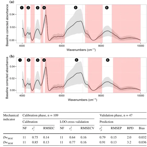
For the 109 samples of the calibration set, the mean MOE was 8211 MPa (i.e N∕mm2) (SD 951 MPa; Table 1). The mean MOR, calculated from 29 of the intact samples, was 41.9 MPa (SD 7.0 MPa). The mean MC was 106%, always greater than 30%. For the 47 samples of the validation set, the mean MOE was 8172 MPa (SD 829 MPa). The mean MC was 113%. For decayed samples, the mean MOE was 3889 MPa and 2966 MPa (SD 2191 and 2486 MPa) for the calibration and validation sets, respectively. The mean MOR was 30.1 and 23.9 MPa (SD 14.2 and 17.1 MPa) for the calibration and validation sets, respectively. For the last series (i.e. 505 degradation days, 25 samples), the MOE and MOR were set at 0 MPa because the samples were too degraded to be tested using bending tests and could easily be broken by hand. The MOE and MOR were correlated in the intact and decayed states (Fig. 4). Indeed, an increase Fig. 3 a Mycelium observed
on the surface of a sample degraded for 73 days. The tape measure is in centimetre. b The mycelium may have a higly variable spatial extent. Sample degraded for 112 days
in MOE induces an increase in MOR. Assuming a linear relationship between these two variables gives coefficients of determination r2 of 0.72 and 0.86, respectively.
The MOE and MOR measurements in decayed condi-tions were skewed by the heterogeneity of fungal decay visually observed in the cross-section given that Eqs. 2 and
3 were defined assuming an isotropic material. However, it gave coherent values from a decay-assessment perspec-tive. Thus, the degradation process tested in the greenhouse provided a large data set of 156 DwMOE and DwMOR
val-ues (Fig. 5). Regarding DwMOR, 28 negative values ranging
from −0.27 to 0 (mean of negative DwMOR: −0.09) were
observed as the MOR of decayed samples was compared to a mean MOR of intact samples. This is in particular the consequence of the MOR’s variability rated at 9 MPa (SD
for silver fir—Tropix 7). From a mechanical point of view, both indicators have different meanings and appear to be complementary in the context of timber structure design and monitoring. DwMOE is related to the bending stiffness
and therefore linked to wooden beam deformation. DwMOE
could therefore be used to assess a capacity of deformation before rupture. DwMOR is related to the bending strength
and thus to the material rupture.
3.2 Near-infrared spectra
Spectrum exploration using PCA performed with all wavenumbers showed a separation between intact and decayed NIRS-samples (Fig. 7a). The first component (PC1) loadings (Fig. 7b) were characterized by three main peaks (around 4502, 5361 and 7577 cm−1) corresponding to wavenumbers where baseline-corrected absorbances are extremely low (Fig. 6). These three peaks were also observed on the second component (PC2) loadings (4995, 5331, 5390, 7553 and 7658 cm−1). The PC2 pointed to a lesser extent to five other wavenumbers: 4142, 4870, Table 1 Physical and
mechanical measurements and indicators of the level of decay
Range and standard deviation (SD)
aMeasured for 29 intact samples
Calibration set, n=109 Validation set, n=47
Wood property Mean Min. Max. SD Mean Min. Max. SD Intact samples Moisture content (%) 106 32 179 44 113 35 181 47 MOEintact (MPa) 8211 5672 10275 951 8172 5792 9460 829 MORintact (MPa)a 41.9 28.3 56.6 7.0 – – – – Decayed samples Moisture content (%) 104 42 175 37 106 47 170 35 MOEdecay (MPa) 3889 0 9001 2191 2966 0 6905 2486 MORdecay (MPa) 29.8 0 53.3 14.2 23.9 0 49.9 17.1 Indicators DwMOE (–) 0.52 0.06 1 0.27 0.64 0.13 1 0.30 DwMOR (–) 0.29 −0.27 1 0.34 0.43 −0.19 1 0.42 0 10 20 30 40 50 0 2500 5000 7500 10000
Modulus of Elasticity [MPa]
Modulus of Rupture [M
Pa
] R² = 0.83
R² = 0.76
Fig. 4 Relationship between the MOE and MOR in intact (black points) and decayed (grey points) states
0 5 10 15 20 0.0 0.4 0.8 Indicators Count DwMOE DwMOR
Fig. 5 Distribution of the mechanical degradation indicators DwMOE
5022, 5770, 9045 cm−1. PCA performed only on decayed NIRS-samples showed a graduation of DwMOE (Fig. 8a)
or DwMOR (Fig. 8b) visible along PC1 axes.
The mean intact and decayed spectra followed the same pattern but decayed spectra had lower baseline-cor-rected absorbance values in the whole NIR spectral range (4000–10,000 cm−1) (Fig. 6).
The findings of this study confirm that NIRS spec-tra contain relevant information regarding the microbial activity in wood, even at the early stage. The first fea-ture highlighted by PCA (Fig. 7a) is a difference between
the spectra of intact and decayed samples, whatever the duration of decay. This is also observed on the spectrum plot (Fig. 9). The loss in baseline-corrected absorbance of decayed spectra compared to the intact spectra is vis-ible in regions associated with cellulose (peaks 5865 and 6727 cm−1) or lignin (peaks, 6875 and 5972 cm−1) (Schwanninger et al. 2011). Similar observations have been described with different wood species decayed by brown or white rots (Fackler et al. 2007a; Sandak et al.
2013), remembering that soft rot may be involved in the current experiment given that the samples were sub-jected to a microbial community. This constant difference 0.00 0.05 0.10 0.15 4000 4500 5000 5500 6000 6500 7000 7500 8000 8500 9000 9500 10000 Wavenumber (cm-1)
Baseline corrected absorbance
Fig. 6 Mean intact spectrum (solid line) and the mean decayed spectra (solid line with ribbon) with the ribbon that represents the absorbance
standard deviation PC1 90.14% PC2 5.19% green nir-samples decayed nir-samples (a) (b) 4000 5000 6000 7000 8000 9000 10000 −1.0 −0.5 0. 00 .5 1.0 Wavenumbers [cm−1] Loadings 4502 5022 5361 5403 5333 7577 7646 9045 7563
Fig. 7 a Principal component analysis of the baseline-corrected
spectra of intact and decayed samples. The ellipses graphically sum-marize the point clouds. b Loadings of the first two principal
compo-nents (dashed and solid lines, respectively). The ribbons correspond to ranges where baseline-corrected absorbance is null
between spectra confirms the value of calculating a dif-ferential spectrum that extracts the meaningful spectral information. PCA of decayed NIRS-samples (Fig. 8) also distinguishes strongly decayed samples (DwMOE > 0.75
and DwMOR > 0.75 ) from samples that are less decayed
along the PC1 axis. PCA is, however, limited for further investigation because of an aggregation of less decayed NIRS-samples. PCA loadings (Fig. 7b) reveal no specific wavelength except one associated with OH-bonds (peak, 5021 cm−1) and others where baseline-corrected absorb-ance is low (peaks, 4502, 5361, 7577 and 9036 cm−1).
The differential spectra provide evidence of some spec-tral regions where differences between the mean intact spectrum and decayed spectra are of interest (Fig. 11). Nev-ertheless, these regions are distributed all along the NIR range. PLSR performed in the whole NIR range should be sufficient to assess decay, as other studies did (Stirling et al.
2007; Leinonen et al. 2008; Green et al. 2012). But this
solution would not be optimal according to suggestions by Nadler and Coifman (2005) and Cécillon et al. (2008) that prescribe wavelength range reduction to decrease the root mean square error of PLSR. This motivated the develop-ment of the wavelength selection method presented in this study.
3.3 Prediction of mechanical degradation indicators
DwMOE and DwMOR using the PLSR of differential
spectra
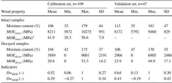
Wavelength selection The optimal SD values to determine wavenumbers ranges optimizing the PLSR are 0.0062 (DwMOE) and 0.0055 (DwMOR) (Fig. 10). Figure 11
pre-sents the different spectral ranges kept for the PLSR. In both cases, six similar ranges were selected. Amongst the six regions identified, regions 2, 3, 4 and 5 of both mod-els (Fig. 11) had similarities to those obtained by other Fig. 8 Principal component
analysis of the baseline-corrected spectra of decayed samples. Grey scale and sizes are a function of the level of decay according to DwMOE (a) and DwMOR (b) −20 −10 0 10 −50 0 50 100 PC1 PC2 0.25 0.50 0.75 1.00 DwMOE −20 −10 0 10 −50 0 50 100 PC1 PC2 −0.25 0.00 0.25 0.50 0.75 1.00 DwMOR
Fig. 9 Mean spectra of intact
(solid line) and decayed (solid
line with ribbon) silver fir
sam-ples. The ribbon corresponds to the standard deviation of decayed sample absorbance. The cellulose spectrum cor-responds to the dashed line and the lignin kraft spectrum corre-sponds to the dotted dashed line
0.00 0.05 0.10 0.15 5500 5750 6000 6250 6500 6750 7000 7250 7500 Wavelength [cm-1]
research on decay effects on wood spectra. Fackler et al. (2007b) found the best regression for weight loss of brown rotted beech wood in the NIR region (7235–6106 and 5384–4150 cm−1). They reported that this model was not applicable to white rot fungi. Ishizuka et al. (2012) retained 4050–5000 and 5800–6800 cm−1 for PLSR to predict lignin and cellulose contents. The main difference between the two studies and the results presented herein remains in the (5800–6000 cm−1) region associated with lignin and identi-fied as being important in the case of white rot. This range was not included in region 5, which starts at 6163 and 6144 cm−1 for Dw
MOE and DwMOR, respectively. It was concluded
that lignin might be less affected than polysaccharides by the fungal community involved. In natural conditions, the composition of the fungal community changes over time and depends on early established and long-lived species (Ottoson 2013). Thus, further investigations of the method
on various fungal communities in natural conditions would be highly valuable.
PLSR models With these spectral ranges, two PLSR models were developed from differential spectra Sdiff to
pre-dict DwMOE or DwMOR. The results obtained after the LOO
validation were significant with RMSECV of 0.16 for both indicators and r2
v of 0.63 and 0.77 for DwMOE and DwMOR
prediction, respectively (Table 2). These models applied to the validation set confirm the consistency of the results: to predict DwMOE and DwMOR, RMSEP was 0.15 and 0.13, r2p
was 0.79 and 0.91, RPD was 2.0 and 3.2, and the bias was 0.032 and 0.036, respectively. The relationships between measured and NIR-predicted values for both indicators and their associated prediction residuals are shown in Fig. 12.
The current results support previous research (Tsu-chikawa and Schwanninger 2013) that reported a statisti-cal link between NIRS spectra and mechanistatisti-cal properties
4000 5000 6000 7000 8000 9000 10000 0.000 0.005 0.010 0.015 Wavenumber Wavenumber standard de viation − [Dw moe] 4000 5000 6000 7000 8000 9000 10000 0.000 0.00 50 .010 0.015 standard de viation − [Dw mor] 0.005 0.006 0.007 0.008 0.009 0.16 50 .170 0.175 0.180 standard deviation RMSEP [Dw moe] 0.005 0.006 0.007 0.008 0.009 0.16 50 .170 0.17 50 .180 0.185 standard deviation RMSEP [Dw mor] (a) (b) (c) (d)
Fig. 10 Standard deviation of the differential spectra Sdiff with the optimal SDlim (dashed lines) for PLSR with DwMOE (a), and with
DwMOR (b). RMSEP variation is a function of SDlim for DwMOE (c)
and for DwMOR (d). The dashed lines correspond to the optimal SDlim, i.e. where RMSEP is minimal
using PLSR. However, while most studies work with intact wood, the current models establish relationships between NIRS differential spectra Sdiff and losses in MOE
and MOR of decayed wood (Table 2). Green et al. (2010a) already used NIRS and PLSR to predict the level of decay in wood measured by compression strength in particular. They obtained appreciable results with r2
p of 0.69 and RPD
of 2.61 (model with raw spectra). While this study showed that NIRS could predict wood decay, it used Gloeophyllum trabeum (brown rot type) to inoculate samples. The cur-rent study shows similar results (r2
p 0.79 and RPD 2.0 for
DwMOE prediction. r2
p 0.91 and RPD 3.2 for DwMOR
predic-tion) for predicting the level of decay in silver fir wooden strips inoculated with a microbial community.
Finally, from a practical standpoint, these methods may be applied to real structures by means of core collection (Noetzli et al. 2008). Spectral acquisition of cores could be directly acquired at different parts of the cores or on milled
cores (Schimleck 2008). Cores 5 mm in diameter have very limited mechanical damage against the diameter of the logs generally used in ecological engineering structures (diame-ter above 150 mm) and are easy to reduce into powder. This would give practitioners quantitative information about the level of decay of parts located by their expertise. However, the method needs to be tested previously on beams simi-lar to those used in ecological engineering structures, i.e. wooden logs. The mean intact spectrum of silver fir should also be enriched by spectra from other locations to ensure that it covers the heterogeneity of the species.
4 Conclusion
The main purpose of this study was to predict degradation indicators of silver fir wooden strips decayed by a micro-bial community using NIRS. Two indicators of the level Fig. 11 Mean spectrum and
standard deviation of the dif-ferential spectra Sdiff. The red
ribbons (lengthwise stripes)
show the excluded wave-numbers for PLSR. a DwMOE prediction, range 1: 3900–4104 cm−1, range 2: 4211–4420 cm−1, range 3: 4632–4929 cm−1, range 4: 5079–5145 cm−1, range 5: 6163–7243 cm−1, range 6: 8080–8539 cm−1. b DwMOR prediction. range 1: 3900–4107 cm−1, range 2: 4200–4423 cm−1, range 3: 4624–4933 cm−1, range 4: 5068–5145 cm−1, range 5: 6144–7343 cm−1, range 6: 8079–8604 cm−1 0.00 0.02 0.04 4000 6000 8000 10000 Wavenumbers (cm−1)
Baseline corrected absorbanc
e 1 2 3 4 5 6 0.00 0.02 0.04 4000 6000 8000 10000 Wavenumbers (cm−1)
Baseline corrected absorbanc
e
1 2 3 4 5 6
(a)
(b)
Table 2 Main model
characteristics developed for predicting indicators DwMOE and DwMOR
NF number of factors, RMSEC root mean squared error of calibration, RMSEC root mean squared error of
cross validation, RMSEP root mean squared error of prediction, RPD relative percent difference ratio of SD to RMSEP, Bias the difference of the mean of the predicted versus the mean of the true values
Mechanical
indicator Calibration phase, n = 109 Validation phase, n = 47 Calibration LOO cross-validation Prediction
NF r2 c RMSEC NF r 2 v RMSECV r 2 p RMSEP RPD Bias DwMOE 11 0.75 0.14 11 0.64 0.16 0.79 0.15 2.0 0.032 DwMOR 11 0.85 0.13 11 0.77 0.16 0.91 0.13 3.2 0.036
of decay, DwMOE and DwMOR, were developed allowing
an accurate evaluation of the level of decay in terms of mechanical properties. These indicators were related to the near infra-red spectra seen as estimators of the chemi-cal compounds. The analysis of the NIRS spectra of intact and decayed milled samples confirmed the NIRS sensitivity to decay even under semi-controlled conditions. This sen-sitivity is observable over the full spectral range and non-attributable to one specific chemical compound (i.e. lignin, cellulose or hemicellulose). Based on these observations, two models were developed from spectra to predict DwMOE
and DwMOR using PLSR. Predicted and measured values
were highly correlated with r2
p values of 0.79 (DwMOE) and
0.91 (DwMOR). These models can provide useful tools for
the rapid screening of wood residual properties of struc-tural members. For that purpose, complementary investiga-tions are needed. The scattering effects may be corrected by several methods, the multiplicative scatter corrections in particular (Rinnan et al. 2009), that should be compared in the context of the assessment of the level of decay. Further-more, the method has been intentionally developed with a
data set of limited variability (samples were sampled from one log). The generalisation of the method with a data set taking into account an extensive variability is necessary. Acknowledgements This work has been financed within the
frame-work of projects SEDALP (Interreg Alpine space program. 2013-2015) and Arc Environnement (Rhône Alpes Region, France).
References
Beleites C, Sergo V (2012) hyperSpec: a package to handle hyper-spectral data sets in R
Bellon-Maurel V, Fernandez-Ahumada E, Palagos B, Roger JM, McBratney A (2010) Critical review of chemometric indica-tors commonly used for assessing the quality of the prediction of soil attributes by NIR spectroscopy. TrAC Trends Anal Chem 29(9):1073–1081
Blanchette RA (1995) Degradation of the lignocellulose complex in wood. Can J Bot 73(S1):999–1010
Cécillon L, Cassagne N, Czarnes S, Gros R, Brun JJ (2008) Vari-able selection in near infrared spectra for the biological char-acterization of soil and earthworm casts. Soil Biol Biochem 40(7):1975–1979
Fig. 12 Comparison between
measured and predicted values for DwMOE (a) and DwMOR (c). The empty dots indicate the calibration set and the filled
dots indicate the validation set.
Prediction residuals DwMOE (b) and DwMOR (d) of for the valida-tion set 0.0 0.2 0.4 0.6 0.8 1.0 0. 00 .2 0.4 0.6 0. 81 .0 DwMOE (measured) Dw MOE (predicted) 0 10 20 30 40 −0.4 −0.2 0. 00 .2 Predictions Residuals r2 v= 0.63 r2 p= 0.79 0.0 0.5 1.0 0. 00 .5 1.0 DwMOR (measured) Dw MOR (predicted) 0 10 20 30 40 −0.3 −0.1 0. 10 .2 0.3 Predictions Residual s r2 v= 0.77 r2 p= 0.91 (a) (b) (c) (d)
CEN (2005) EN 1995-1-1. Eurocode 5—design of timber struc-tures—Part 1-1—General rules: general rules and rules for buildings. Tech. rep., Brussels, Belgium
CEN (2014) EN 252:2013. Field test method for determining the rela-tive protecrela-tive effecrela-tiveness of a wood preservarela-tive in ground contact. Tech. rep., CEN, Brussels, Belgium
CIRAD (2011) Tropix 7 version 7.5.1. doi:10.18167/74726f706978
Curling S, Clausen C, Winandy J (2002) Relationships between mechanical properties, weight loss, and chemical composi-tion of wood during incipient brown-rot decay. For Prod J 52(7–8):34–39
Dackermann U, Crews K, Kasal B, Li J, Riggio M, Rinn F, Tannert T (2013) In situ assessment of structural timber using stress-wave measurements. Mater Struct 47(5):787–803
Dinwoodie JM (2000a) Deformation under load. In: Timber: its nature and behaviour, 2nd edn. CRC Press, p 274
Dinwoodie JM (2000b) Strength and failure in timber. In: Timber: its nature and behaviour, 2nd edn. CRC Press, p 274
Fackler K, Schwanninger M (2012) How spectroscopy and micro-spectroscopy of degraded wood contribute to understand fungal wood decay. Appl Microbiol Biotechnol 96(3):587–599
Fackler K, Schmutzer M, Manoch L, Schwanninger M, Hinterstoisser B, Ters T, Messner K, Gradinger C (2007a) Evaluation of the selectivity of white rot isolates using near infrared spectroscopic techniques. Enzyme Microb Technol 41(67):881–887
Fackler K, Schwanninger M, Gradinger C, Hinterstoisser B, Messner K (2007b) Qualitative and quantitative changes of beech wood degraded by wood-rotting basidiomycetes monitored by Fourier transform infrared spectroscopic methods and multivariate data analysis. FEMS Microbiol Lett 271(2):162–169
Fackler K, Schwanninger M, Gradinger C, Srebotnik E, Hinterstoisser B, Messner K (2007c) Fungal decay of spruce and beech wood assessed by near-infrared spectroscopy in combination with uni- and multivariate data analysis. Holzforschung 61(6):680–687 Gonzalez-Rodrigo B, Esteban L, de Palacios P, Garca-Fernndez
F, Guindeo A (2013) Variation throughout the tree stem in the physical-mechanical properties of the wood of Abies alba Mill. From the Spanish Pyrenees. Madera Bosques 19(2):87–107 Green B, Jones PD, Nicholas DD, Schimleck LR, Shmulsky R
(2010a) Non-destructive assessment of Pinus spp. wafers sub-jected to Gloeophyllum trabeum in soil block decay tests by dif-fuse reflectance near infrared spectroscopy. Wood Sci Technol 45(3):583–595
Green B, Jones PD, Schimleck LR, Nicholas DD, Shmulsky R (2010b) Rapid assessment of southern pine decayed by G. tra-beum by near infrared spectra collected from the radial surface. Wood Fiber Sci 42(4):450–459
Green B, Jones PD, Nicholas DD, Schimleck LR, Shmulsky R, Dahlen J (2012) Assessment of the early signs of decay of Pop-ulus deltoides wafers exposed to Trametes versicolor by near infrared spectroscopy. Holzforschung 66(4):515–520
Haines D, Leban JM, Herb C (1996) Determination of Young’s mod-ulus for spruce, fir and isotropic materials by the resonance flex-ure method with comparisons to static flexflex-ure and other dynamic methods. Wood Sci Technol 30(4):253–263
Ishizuka S, Sakai Y, Tanaka-Oda A (2012) Quantifying lignin and holocellulose content in coniferous decayed wood using near-infrared reflectance spectroscopy. J For Res 19(1):233–237 Kasal B, Tannert T (eds) (2011) In situ assessment of structural
tim-ber, RILEM state of the art reports, vol 7. Springer, Dordrecht Kelley SS, Jellison J, Goodell B (2002) Use of NIR and
pyrolysis-MBMS coupled with multivariate analysis for detecting the chemical changes associated with brown-rot biodegradation of spruce wood. FEMS Microbiol Lett 209(1):107–111
Kelley SS, Rials TG, Groom LR, So CL (2004) Use of near infrared spectroscopy to predict the mechanical properties of six soft-woods. Holzforschung 58(3):252–260
Leinonen A, Harju AM, Venlinen M, Saranp P, Laakso T (2008) FT-NIR spectroscopy in predicting the decay resistance related char-acteristics of solid Scots pine (Pinus sylvestris L.) heartwood. Holzforschung 62(3):284–288
Liland KH, Mevik BH (2014) Baseline: baseline correction of spectra Mevik BH, Cederkvist HR (2004) Mean squared error of predic-tion (MSEP) estimates for principal component regression (PCR) and partial least squares regression (PLSR). J Chemom 18(9):422–429
Mevik BH, Wehrens R, Liland KH (2013) pls: partial least squares and principal component regression
Mkip R, Linkosalo T (2011) A non-destructive field method for measuring wood density of decaying logs. Silva Fennica. doi:10.14214/sf.91
Nadler B, Coifman RR (2005) The prediction error in CLS and PLS: the importance of feature selection prior to multivariate calibra-tion. J Chemom 19(2):107–118
Noetzli K, Boell A, Graf F, Sieber T, Holdenrieder O (2008) Influ-ence of decay fungi, construction characteristics, and environ-mental conditions on the quality of wooden check-dams. For Prod J 58(4):72–79
Ottoson E (2013) Succession of wood-inhabiting fungal communi-ties. PhD thesis, Swedish University of Agricultural Sciences, Uppsala
Previati M, Canone D, Bevilacqua I, Boetto G, Pognant D, Ferraris S (2012) Evaluation of wood degradation for timber check dams using time domain reflectometry water content measurements. Ecol Eng 44:259–268
Przewloka SR, Crawford DM, Rammer DR, Buckner DL, Woodward BM, Li G, Nicholas DD (2008) Assessment of biodeterioration for the screening of new wood preservatives: calculation of stiff-ness loss in rapid decay testing. Holzforschung 62(3):270–276 R Core Team (2013) R: a language and environment for statistical
computing
Rinnan Å, van den Berg F, Engelsen SB (2009) Review of the most common pre-processing techniques for near-infrared spectra. TrAC Trends Anal Chem 28(10):1201–1222
Rowell R (2012) Chemistry of wood strength. In: Handbook of wood chemistry and wood composites. CRC Press, p 703
Sandak A, Ferrari S, Sandak J, Allegretti O, Terziev N, Riggio M (2013) Monitoring of wood decay by near infrared spectroscopy. Adv Mater Res 778:802–809
Sandak A, Sandak J, Riggio M (2015a) Assessment of wood struc-tural members degradation by means of infrared spectroscopy: an overview. Struct Control Health Monit. doi:10.1002/stc.1777
Sandak J, Sandak A, Riggio M (2015) Multivariate analysis of multi-sensor data for assessment of timber structures: principles and applications. Constr Build Mater 101(Part 2):1172–1180 Schimleck L (2008) Near-infrared spectroscopy: a rapid
non-destruc-tive method for measuring wood properties and its application to tree breeding. N Z J For Sci 38(1):14–35
Schimleck LR, Mora C, Daniels RF (2003) Estimation of the physi-cal wood properties of green Pinus taeda radial samples by near infrared spectroscopy. Can J For Res 33(12):2297–2305 Schwanninger M, Rodrigues JC, Fackler K (2011) A review of band
assignments in near infrared spectra of wood and wood compo-nents. J Near Infrared Spectrosc 19(5):287–308
Schwarze FWMR (2007) Wood decay under the microscope. Fungal Biol Rev 21(4):133–170
Sila A, Terhoeven-Urselmans T (2013) soil.spec: soil spectral file conversion, data exploration and regression
Stirling R, Trung T, Breuil C, Bicho P (2007) Predicting wood decay and density using NIR spectroscopy. Wood Fiber Sci 39(3):414–423
Stokland JN, Siitonen J, Jonsson BG (2012) Biodiversity in dead wood. Ecology, biodiversity, and conservation. Cambridge Uni-versity Press, New York
Tsuchikawa S, Schwanninger M (2013) A review of recent near-infra-red research for wood and paper (Part 2). Appl Spectrosc Rev 48(7):560–587
Wilcox W (1978) Review of literature on the effects of early stages of decay on wood strength. Wood Fiber Sci 9(4):252–257
Wold S, Sjstrm M, Eriksson L (2001) PLS-regression: a basic tool of chemometrics. Chemom Intell Lab Syst 58(2):109–130