UNIVERSITÉ DU QUÉBEC À MONTRÉAL
CHARACTERISATION OF MULTI-MODEL ENSEMBLES OF
CLIMATE-CHANGE PROJECTIO S REGARDING SAMPLING, TREATMENT AND INTERPRETATION
THESIS
PRESENTED
AS PARTIAL REQUIREMENT
FOR PHD DEGREE IN EARTH A D ATMOSPHERIC SCIENCES
BY
MARTIN LEDUC
Avertissement
La diffusion de cette thèse se fait dans le respect des droits da son auteur, qui a signé le formulaire Autorisation de reproduire et de diffuser un travail de recherche de cycles supérieurs (SOU-522- Rév.01-2006). Cette autorisation stipule que «conformément
à
l'article 11 du Règlement no 8 des études de cycles supérieurs, [l'auteur] concèdeà
l'Université du Québecà
Montréal une licence non exclusive d'utilisation et de publication de la totalité ou d'une partie importante de [son] travail de recherche pour des fins pédagogiques et non commerciales. Plus précisément, [rauteur] autorise l'Université du Québec à Montréal à reproduire, diffuser, prêter, distribuer ou vendre des copies de [son] travail de recherche à des fins non commerciales sur quelque support que ce soit, y compris l'Internet. Cette licence et cette autorisation n'entraînent pas une renonciation de [la] part [de l'auteur]à
[ses] droits moraux nià
[ses] droits de propriété intellectuelle. Sauf entente contraire, [l'auteur] conserve la liberté de diffuser et de commercialiser ou non ce travail dont [il] possède un exemplaire.»CARACTÉRISATION DES ENSEMBLES MULTI-MODÈLES DE PROJECTIONS DES CHANGEMENTS CLIMATIQUES AU NIVEAU DE L'ÉCHANTILLONNAGE, DU TR.AITEME TET DE L'INTER.PR.ÉTATIO J
THÈSE
PRÉSENTÉE
COMME EXIGE CE PARTIELLE
DU DOCTORAT EN SCIE CES DE LA TER.R.E ET DE L'ATMOSPHÈRE
PAR.
MARTIN LEDUC
Je voudrais tout d'abord remercier mon directeur de recherche, René Laprise, pour ses valeurelL"X conseils scientifiques, pour sa grande générosité ainsi que pour la liberté qu'il m'a donnée dans l'élaboration de ce projet de doctorat.
Je tiens aussi à remercier Ramon de Elia qui m'a beaucoup aidé autant d'un point de vue scientifique que personnel ainsi que Léo Séparovic pour les discussions philosophiques et son aide en mathématiques. Aussi, merci à Barbara Casati pour ses commentaires précieux et à Alejandro Di Luca pour sa participation à l'analyse des résultats. Merci au personnel du centre ESCEn. eL du consortium Ouranos de m'avoir permis de travailler dans un environnement stimulant et enrichissant. De plus, je tiens à remercier le centre ESCER ainsi que le programme de Fonds à l'Accessibilité et à la réussite des Études (FARE) de l'UQAM pour le financement accordé au cours de mes études.
Merci à Mélissa pour son amour, sa compréhension, pour m'avoir inspiré et ac-compagr:é tout au long de mon doctorat. Finalement, merci à mes parents et mes amis pour leur soutien moral via les plaisirs de la vic.
LIST OF FIGURES LIST OF TABLES . LIST OF ACRONYMS RÉSUMÉ . . ABSTRACT INTRODUCTION CHAPTER I
ON THE UNCERTAINTY RELATED TO EXPERTS' DECISIONS IN THE SE-LECTION OF A SUBSET OF SIMULATIONS FROM A LARGE ENSEMBLE
xi xvii xix xxi niii 1 OF OPPORTUNITY 11 1.1 1.2 1.3 Introduction . Experimental Framework
1.2.1 Data and pre-processing . 1.2.2 Ensemble statistics . 1.2.3 Member sampling 1.2.4 Mode! sampling . Results
1.3.1 Signal, spread and their uncertainties 1.3.2 Smaller ensemble of opportunity 1.3.3 Revisiting the plume diagram . . 1.3.4 Constraining the selection process
11 15 15 16 17 19 20 20 23 27 29 1.4 Discussion and conclusions . . . . . . . . 32 Appendix l.A : Perfect-ensemble experiment for bias correction in the statistics
related to an unbalanced design . . . . . . . . . . . . . . . . . . . . . 41 CHAPTER II
INVESTIGATING CONSENSUSES IN CLIMATE-CHANGE PROJECTIONS FOR MODELS DEVELOPED BY A SAME RESEARCH INSTITUTE . . . . . 59
2.1 Introduction . . . . . . . . . . . . . . . . . . . . 2.2 On the sampling process of an ensemble of opportunity . 2.3 Performance of climate models .
2.4 Independence of climate models .
2.5 Typical differences between models developed by an institute and how this 60 63 64 66
affects their climate-change projections . . . . . . . . . . . . . . . . . . . 70 2.6 Notes on the minimal requirements to the participating centres of a climate
change assessment . . . . . 76
2.7 Discussion and conclusions . 77
Appendix 2.A : Statistical significance of the difference between two ensemble means ( t-test) . . . . . . . . . . . . . . . . . . . . . . 83 CHAPTERIII
THEORETICAL FRAMEWORK FOR RECONSTRUCTING MISSING
MEM-BERS IN A MULTI-MODEL ENSEMBLE OF AOGCMS 93
3.1 Introduction . . ..
3.2 General approach to member reconstruction 3.3 Experimental framework . 3.3.1 Data . 3.3.2 Components of variance 3.3.3 Hypotheses testing 3.4 Results . . . .. 93 96 100 100 100 101 102
3.4.1 Ergodicity in single-mode! ensembles 102
3.4.2 Inter-mode! differences in the simulated total climate variability . 105
3.5 Discussion and conclusions .. . . 107
Appendix 3.A : Applying the ergodic assumption to climate model simulations 109 Appendix 3.B : Approaching stationary conditions by detrending the ensemble mean110 Appendix 3.C Testing the ergodic assumption for a single-mode! ensemble 112 Appendix 3.D Testing the inter-mode! differences in the simulated total climate
variability . . . . . . . . . . . . . . . . . . . . . . . . . . . . . . . . . . . . . 114 CHAPTER IV
4.1 Introduction . . . .. . . . 4.2 Theoretical summary : Review of concepts
127 131 4.2.1 Pre-selection of the simulations . . . 131 4.2.2 Initial sampling of an ensemble of opportunity 132 4.2.3 The ergodic assumption as a workaround for unbalanced ensemble
frameworks . . . . . . . . . . . . . . . . . . . . . . 133 4.2.4 Analysis of variance and decomposition of the uncertainty 134 4.3 Example 1 : Multi-model combination of lhe simulated natural variability 135 4.3.1 Results . . . . . . . . . . . . . . . . . . . . . 138 4.4 Example 2 : Improving statistical testing of the same-institute assumption
based on ergodicity in single-mode! ensembles 142 4.4.1 Results
4.5 Conclusions . .
145 147 Appendix 4.A : Analysis of variance applied to a multi-model ensemble (MME) 155 Appendix 4.B : Assessing the natural variabiliLy by using the member-sampling
method . 157
CONCLUSION 169
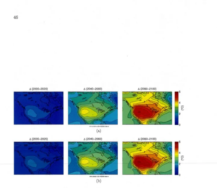
1.1 Signal mean value of climate change caJculated using a) the member sam-pling (6.mem) and b) the mode! sampling (6.mod) methods for the summer surface air temperature over North America for three time periods (from left to right) : 2000-2020, 2040-2060 and 2080-2100 relatively to the 1900-1950 period. AU the available simulations are used in the computation. 46 1.2 Uncertainty of the signal mean value clue to a) the member sampling
(U~em) and b) the mode! sampling (U,~
0
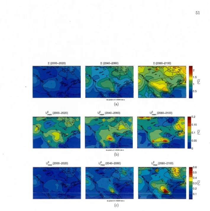
d). AU the available simulations are usee! in the computation. . . . . . . . . . . . . . . . . . . . . . . 47 1.3 Inter-mode! spread mean value calculated using a) the membet sampling(:Emem) and b) the mode! sampling ("Emod). AU the available simulations are used in the computation. . . . . . . 4 7 1.4 Uncertainty of the inter-mode! spread mean value due to a) the member
sampling (UJ.em) and b) the mode! sampling (UJ;.0d). AU the available simulations are used in the computation. . . . . . . . . . . . . 48 1.5 a) Signal mean value (6.) and its components ofuncertainty clue to b) the
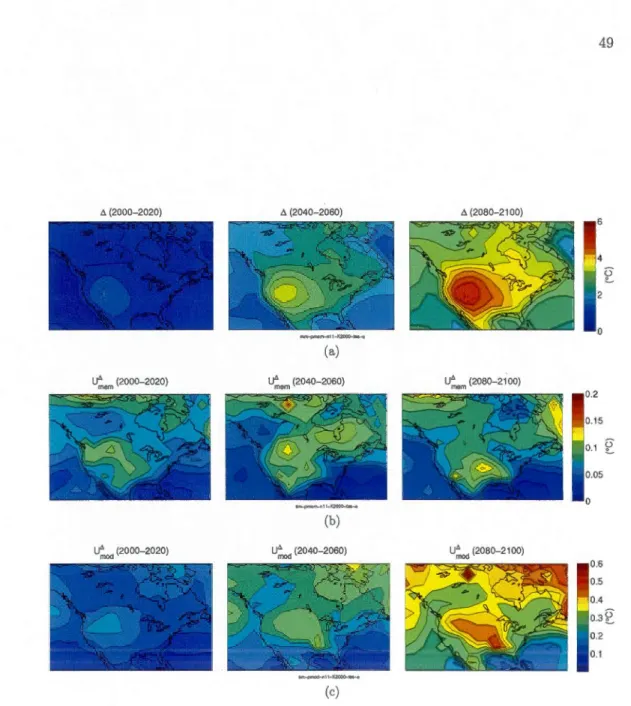
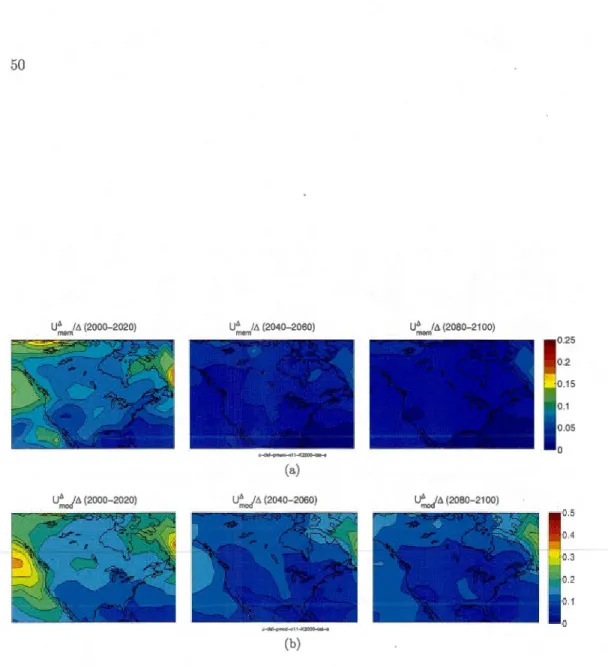
member sampling (U~em) and c) the mode! sampling (Ur~od), calculated using the 11-model subset. . . . . . . . . . . . . . . . . . . . 49 1.6 Relative uncertainty of the signal mean value due to a) the member
sam-pling (U~em/6.) and b) the mode! sampling (U~od/6.), calculated using the 11-model subset. . . . . . . . . . . . . . . . . . . . . 50 1.7 a) Inter-mode! spread mean value (E) and its components of uncertainty
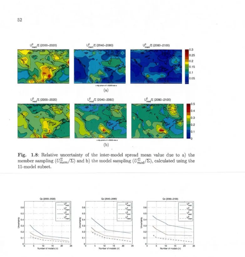
due to b) the member sampling (U,~em) and c) the mode! sampling (UJ;.0d), calculated using the 11-model subset. . . . . . . . . . . . . . . . 51 1.8 Relative uncertainty of the inter-mode! spread mean value clue to a) the
member sampling (UJ.em/E) and b) the mode! sampling (U~od/E), cal-culated using the 11-model subset. . . . . . . . . . . . . . . . . . . 52 1.9 Uncertainty components for the signal and the spread as function of the
number of models in the ensemble for a grid point located at the centre of the Québec province of Canada. . . . . . . . . . . . . . . 52
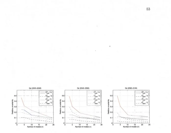
1.10 Relative uncertainty components for the signal and the spread as function of the number of models in the ensemble for a grid point located at the centre of the Québec province of Canada. . . . . . . . . . . . . . 53 1.11 Plume diagram for the surface air temperature in the summer season over
a grid point centred over the Québec province of Canada. The blue and red full !ines consist in the signal and inter-mode! spread mean values respectively, the blue and red dashed !ines are the statistical uncertainty of the signal and inter-mode! spread mean values using the mode! sarn -pling rnethod, and the dotted !ines the statistical uncertainties using the member sampling rnethod. The plumes are obtained from three different ensemble sizes : a) the en tire 24-mode! ensemble and the b) 11-mode! and c) 5-model subsets. . . . . . . . . . . . . . . . . 54 1.12 a) The standard deviation of the mean as function of the sample size
obtained from a synthetic data set generated using a random number ge -nerator based on a normal distribution with zero mean and unit variance. The initial data set consists in 24 elements over which is applied the model-sampling approach by allowing and forbidding mode! replacement (blue and green curves respectively). The curves are normalised using the standard deviation of the initial data set and comparee! with the nonna -lised standard error relationship (in red) clefined as 1/
,;m.
b) The ratio of the errors given by the green and blue curves in (a). . . . 55 1.13 a) The number of combinations that can be formed from an ensemble of24 models as function of the sample size. In green is shown the number of the combinations that can be formed without replacement. The blue curve represents the total number of combinations, including both with and without replacement possibilities. The blue curve is based on the fact that (N~;:-1) multisets of size m can be formed from a pool of N elements while the green curve represents the (~) possible subsets. b) The ratio of the numbers given by the green and blue curves in (a). . . . . . . . . . 56 1.14 The "MME mask" where the black elements (''TRUE" values in the code)
represent the CMIP3 simulations using the A1B scenario and the white elements ("FALSE") stand for Lhe missing simulations in the ensemble compared to the perfect matrix P. Models are distributed along the ho -rizontal axis and the members along the vertical one. . . . . . . . . . 57 1.15 Distribution of the uncertainty cmerging from the member-sampling
ap-proach for the perfect
(U,/;,fm
..
lcft panel) and imperfect(U,/;,e.fn,
right pa-nel) matrices. Frequencies are nonnalised to obtain an integral of 1 under each distribution. . . . . . . . . . . . . . . . . . . 571.16 Distributions of the bias-correction factor ( G) for ensembles of 24, 11,10, 5 and 3 models. Frequenci s are nonnalised to obtain an integral of 1 under each distribution. . . . . . . . . . . . . . . . . . . . 58 2.1 Schematic of the conceptual relationship between prior and posterior
de-finitions of mode! independence. . . . . . . . . . . . . . . . . . . . 87 2.2 Climate-change projections for the a) summer and b) winter surface air
temperature and for the c) summer and d) winter precipitatioü rate. These changes are calculated over 20-year time periods compared to the 1900-1950 leve! for each of the models prcsented in Tab. 2.2. All available realisations are averaged over the regional domain of North America. . . 88 2.3 Difference of the ensemble mean climaLe-change signal for different pairs
of models (or versions) developed by the same research institute. The climate-change signal is calculated for each simulation relatively to the 1900-1950 period. The panel at the boLtom of each difference shows the mask of rejection of the nul! hypothesis by using a two-tailed t-test at the 5% significance leve! (2.5% on each side). Red and blue colours mean positive and negative differences respecLively. . . . . . . . . . 91 3.1 Theoretical framework for an educated guess in the selection of a
member-reconstruction method to be applied to a multi-model ensemble (MME) under transient forcing.
3.2 Single-mode! ensemble schematised as a matrix (X) of time periods. The index t represents the Nr time periods and k represents the NI<
realisa-118
tions (or members) that differ in the i11iLial conditions. . . . . . . . 119 3.3 Testing the ergodic assumption (Hgrgo) using a one-sided F-test at the
10% significance leve!. The colored areas indicate where Hgrgo is rejected over the domain. The ratio of variance (H, see Appendix 3.C) is shown in order to appreciate the physical significance when the ergodic assumption is rejected. The results are shown for the simulations over the 20th century with a climatic time period of 1 year (Nr
=
100) and the models are labeled from the largest (panel a) to the smallest (panel k) single-mode!ensemble size (NK) according to Tab. 3.1. 119
3.4 Idem to Fig. 3.3 but for the 2lst century.
3.5 Relative error of variance (P2) as funcLion of the variance ratio (F2) of the total climate variability as simulaLed by two models (see Appendix
120
3.6 Cross-mode! comparison in the simulated total climate variability over the 20th century. The comparison is based on a two-tailed F-test at the 10% significance leve!. . . . . . . 122 3.7 Idem to Fig. 3.6 but for the 21sl century. 123 3.8 Coefficient of determination (R2) obtained for the fit of a 4th degree
po-lynomial function to the ensemble mean of the GISS-ER mode!. . . 124 3.9 Examples of time series for the four realisations (thin colored !ines) ava
i-lable for the GISS-ER mode!. The series are shown for two grid point located over a) the Atlantic Ocean and b) the Labrador Sea. The black !ines represent the ensemble mean and the red line the 4th degree poly -nomial fit to the ensemble mean. . . . . . . . . . . . . . . . . . 124 3.10 Domain averaged (over North-America) time series of surface air
tempe-rature covering the 1900-2100 period under the A1B scenario for the 11 AOGCMs of the multi-model ensemble (Tab. 3.1). In each panel are shown the available realisations (col01·cd thin !ines), the single-mode! ensemble mean (black) and the polynomial fit (thick red). . . . . . . 126 4.1 Assessing the natural variability from a multi-model ensemble by using
different estimators based on the inter-member spread : a) the weighted inter-member spread (ôwi; ANOVA mean-square error), b) the unweig h-ted inter-member spread (ô-u I), c) the member-sampling estimator (ô-mem) and d) the empirically corrected member-sampling estimator (G x Ô"mem)· 161 4.2 Assessing the natural variability from a multi-model ensemble where each
single-mode! ensemble is reconslructed up to 100 members based on the single-mode! pooling (SMP) melhod : a) the member-sampling estimator
(ô-mem) and b) the ANOVA coefficient (ô-wJ). . . . . . . . . . . . . . . . 162 4.3 Assessing the natural variability from a multi-model ensemble by using a)
weighted ( ô-wTJ) and b) unweighted ( ô-uTJ) time-averaged inter-member spreads. . . . . . . . . . . . . . . . . . . . . . . . . . . . . . . . . 162 4.4 Assessing the natural variability from a multi-model ensemble by using
a) weighted (ôwE) and b) unwcighted (ô-uE) ergodic variances. . . . 162 4.5 Ratio between the different estimates of the natural variability relatively
to a reference estima tor a) the uuweighted inter-member spread ( ô-u I) and b) the unweighted time-averagcd inter-member spread ( ô-uTI). Dist ribu-tions are constructed using dctla from all grid poinls of the domain and all available 20-year average windows from 1900 to 2100. . . . . . 163
4.6 Difference of the ensemble mean climate-change signal for different pairs of models (or versions) developed by the same research institute. The climate-change signal is calculated for cach simulation relatively to the 1980-2000 periocl. The panel at the bottorn of each difference shows the mask of rejection of the nul! hypothesis by using a two-tailed t-test at the 5% significance leve! (2.5% on each side) based on the ergodic assumption.
xv
1.1 Multi-model ensemble formed by 24 AOGCMs taken from the PCMDI archive, which provide climate-change projections based on the A lB emis-sion scenario. The sarnple size (Ni) concsponds to the number of members available for the ith mode! for a total of 55 runs. For more information about models' names and specifications, the reader is invited to refer to the PCMDI website at http: 1 /www-pcmdi .llnl. gov. . . . . . . 45 2.1 Name of the research institutes/groups that provided severa! models or
versions to the CMIP3 multi-model archive. . . . . . . . . . . . . 85 2.2 Table of the main structural, pa.ra.metcrs and numerical differences
bet-ween pairs of models developed by a. same research institute within the CMIP3 mu! ti-mode! archive. Models are compared according to their main components : atmosphere (A), ocean (0), sea ice (I), coupling (C) and land surface (L). The differences are categorised as resolution (R), version (V), mode! (M) and no change (-). . . . . . . . . . . . . . . . . . 85 2.3 Feasibility of a t-test for the difference between ensemble means of
dif-ferent pairs of rnodels, according to the number of simulations available for the AlB scenario within the CMIP3 multi-model dataset. Sample sizes of the two models in a pair are denoted by N x and Ny. In the last column (t), the pairs are denoted by "0" when the test can not be performed, by "E" when equal variances have to be assumed and by "U" when unequal variances can be considered. . . . . . . . . . . . . . . . . . 86 3.1 Names of the models in the CMIP3 multi-model dataset that provide two
or more realisations following the AlB emission scenario. Is also given the number of realisations (Nx) thal arc available for each mode!. For supplementary information, the reader is invited to refer to the PCMDI website at http: 1 /www-pcmdi .llnl. gov. . . . . . . . . . . . . . . . 117 3.2 One-way analysis of variance table whcrc the total sum of squares, the
treatment sum of squares and the sum of squared errors are expressed with their respective number of degrees of freedom. Nrr is the number of time periods and N K is the number of realisations generated using the climate mode!. . . . . . . . . . . . . . . . . . . . . . . . 117
ANOVA AOGCM AR4 CMIP3 EPP GESA GHGA GIEC IPCC MCGAO MMD MME MMP NARCCAP PC MDI PPE RCM SDM SMP SRES TAR Analysis of Variance
Atmosphere-Ocean General Circulation Mode! IPCC Fourth Assessment Report
Coupled Mode! Intercomparison Project phase 3 Ensemble à la physique perturbée
Gaz à effet de serre et aérosols Greenhouse Cases and Aerosols
Groupe d'experts intergouvernemental sur l'évolution du climat Intergovernmental Panel on Climate Change
Modèle de Circulation Générale Couplé Atmosphère-Océan CMIP3 Multi-Model Dataset
Multi-Model Ensemble Multi-:tvlodel Pooling
The North Arnerican Regional Climate Change Assessment Program Program for Climate Mode! Diagnosis and Intercomparison
Perturbcd Physics Ensemble Regional Climate Mode! Statistical Downscaling Mode! Single-Mode! Pooling
Special Report on Emissions Scenarios IPCC Third Assessment ReporL
Cette thèse traite de diverses difficultés inhérentes à l'analyse d'ensembles multi -modèles de projections de changements climatiques. Ces ensembles, souvent appelés « ensembles d'opportunité », sont formés en fonction de la disponibilité de plusieurs centres de modélisation à l'échelle mondiale à produire un certain nombre de simulations. Les ensembles résultants d'un tel processus ne sont donc pas construits selon un cadre expérimental systématique visant à permettre une analyse optimale, mais plutôt en fonction de facteurs externes émergeant d'un processus d'échantillonnage ouvert.
Dans le premier chapitre de cette thèse, le concept d'un échantillonnage de type «expert» est étudié. Consistant en une présélection d'un certain nombre de simulations à partir de l'ensemble disponible, ce type de processus est généralement utilisé dans le but de réduire la taille d'un ensemble qui ne peut être traité en entier lorsque les res-sources sont limitées. Les incertitudes d'échantillonnage reliées au calcul des statistiques de l'ensemble sont calculées en ré-échantillonnant sur un grand nombre de sous-ensembles de simulations. Le processus de sélection est divisé en deux types de choix faits par les experts : le choix des modèles et celui des membres. Il est démontré comment ces in-certitudes d'échantillonnage consistent en des manifestations de sources d'incertitudes connues reliées aux projections climatiques, soient la variabilité climatique naturelle et l'écart-type inter-modèle.
Le second chapitre vise à étudier une problématique fondamentale à l'échantillon-nage des modèles dans un ensemble d'opportunité. Les modèles de climat n'étant a priori pas tout à fait indépendants puisque les scientifiques partagent des connaissances à propos du système climatique et quant à la manière de construire les modèles, au-cune métrique pour évaluer cette indépendance ne fait présentemenL consensus entre les scientifiques. Dans ce chapitre, nous proposons un critère pour déLecter un manque d'indépendance entre les projections de changements climatiques. Ce critère est basé sur le fait que deux modèles peuvent mener à des scnsihilités climatiques similaires face atLx forçages externes, mais un tel consensus devrait être rejeté quand des raisons suffisantes peuvent remettre en cause la notion d'indépendance. Par exemple, lorsque d'importantes similarités structurelles apparaissent entre les modèles ou, dans une moindre mesure, dû à une certaine dépendance institutionnelle.
Dans le troisième chapiLre, des pistes de solutions sont suggérées face au problème que les modèles sont généralement représentés da.ns un ensemble par peu de membres et en nombres souvent inégaux. L'utilisation d'échantillons non-équilibrés peut engendrer certains problèmes, particulièrement en ce qui a trait à l'estimation de la variabilité natu-relle dans l'ensemble, celle-ci étant souvent obtenue à partir de l'écart-type inter-membre.
Avant de considérer des méthodes de reconstruction visant à régénérer les simulations jugées manquantes à partir de l'information disponible dans l'ensemble, deux hypothèses se doivent d'être vérifiées. La première s'applique à un ensemble de membres provenant d'un seul modèle et consiste à déterminer si cet ensemble peut être supposé comme étant ergodique, c.-à-d. que la variabilité temporelle est à peu près égale à celle qui intervient entre les membres. La seconde hypothèse considère que la variabilité naturelle est s imu-lée de façon égale entre les modèles. Bien que les résultats montrent que la variabilité naturelle diffère de façon importante entre les modèles, l'hypothèse d'ergodicité entre les membres s'avère vraie pour des simulations sans forçages externes. Pour des simulations avec forçages externes, il est démontré comment des conditions de stationnarité peuvent être atteintes par traitement en soustrayant les tendances polynomiales dans les séries temporelles.
Dans le quatrième chapitre sont cornparées différentes méthodes pour quantifier la variabilité naturelle à partir d'une combinaison de plusieurs modèles. D'un côté, l'estimé optimal pour cette variabilité serait biaisé vers les modèles avec le plus de membres, tan-dis qu'un estimé donnant le même poids à tous les modèles serait caractérisé par une plus grande erreur type. Dans ce même chapitre est aussi fourni un exemple d'application de l'hypothèse d'ergodicité, qui permet d'utiliser la variabilité temporelle afin de comparer les signaux de changements climatiques provenant de deux modèles, lorsque ces derniers sont représentés par un seul membre. Cette approche peut être vue comme une alte r-native devant la méthode plus coûteuse de considérer des expériences supplémentaires, par exemple les simulations de contrôle pour la période préindustrielle disponibles dans l'ensemble CMIP3.
Mots clés : ensemble multi-modèle, échantillon non balancé, variabilité naturelle, ince r-titude modèle, indépendance des modèles, ergodicité
This thesis focuses on inherent issues to the analysis of multi-model ensembles of climate-change projections. Such ensembles, oftcn denoted as "ensembles of opportunity", are formed on the basis of the readiness of severa! modelling centres around the world to produce simulations. It results in ensembles Lhat are not constructed based on a systematic framework aimed at an optimised analysis but rather on external factors emerging from an open sampling process.
In the first chapter of this thesis, the concept of an expert-based sampling is in-vestigated, consisting in making a pre-selection of a number of simulations from a large ensemble. Such a sampling process is generally used by research centres that cannot afford to handle the entire ensemble due to limited resources of treatment. Sampling un-certainties affecting the statistics of the resulting ensemble are assessed using resampling methods by randomly selecting over severa! ensembles subsets. The selection process is divided as two types of choices made by the experts : the choice of the models and that of the members. We show how these sampling uncertainties are manifestations of known sources of uncertainty, namely the natural climate variability and the inter-mode! spread.
The second chapter investigates an issue that is fundamental to the sampling of the models in an ensemble of opportunity. Whilc clima.te models are not expected to be independent since scientists share knowledge about the climate system and on how to construct models, no robust metric to qua.ntify mode! independence is commonly accepted among climate scientists. In this cha.pter, we propose a criterion for detecting possible la.ck of independence between elima te-change projections. This cri teri on is ba.sed on the fact that two models can lead to similar clirnate sensitivities to external forcings, but such a consensus should be rejected when there are sufficient reasons to believe that it occurs for the wrong reasons, i.e. whether duc to important structural similarities between the models or to a lesser extent, to some institutional dependence.
In the third chapter, a workaround to the apparent problem of a small and une-quai number of members provided by the models is investigated. Such an imbalance between sample sizes mises issues in the assessment of the natural climate variability when obtained from the inter-member spread. \Vhcn considering reconstruction methods for regenerating these "missing simulations", two assumptions about Lhe multi-model en-semble have to be investigated. The first one applies to a single mode! and consists in determining whether an ensemble of members can be a..ssumed as ergodic, i.e. that the variability measured in time is approximately equal to the inter-member spread. The second assumption is that the natural variability is equally simulated by the different
under stationary conditions. For simulations run under transient forcings, it is shown how stationary conditions can be reached by treatment by removing polynomial trends from the time series.
In the fourth chapter, different methods are compared for assessing the natural variabilit-y from a multi-model ensemble. While an optimal estimator of the natural va-riability would be biased toward the models with larger sample sizes, an unweighted estimate that gives an equal importance to the different models would be affected by larger sampling en·ors. We also provide an example of application of the ergodic assump-tion that allows taking advantage of the temporal variability in the simulations in order to compare the climate-change signais provided by two models when both provide a single member. This method can be seen as an alternative to the more expensive way of using supplementary simulations run without external forcings such as the pre-industrial control experiments in the CMIP3 multi-model ensemble.
Keywords : multi-rnodel ensemble, unbalanced framework, natural variability, mode! uncertainty, mode! independence, ergodicity
La méthode scientifique requiert que les théories soient validées par l'expérimentation. Toutefois, en science du climat, les chercheurs n'ont pas accès à un laboratoire au sens classique qui permette de vérifier leurs hypothèses. En ce sens, le système climatique terrestre est à la fois laboratoire et sujet d'étude. Considérant que certaines perturbations du système climatique peuvent prendre plusieurs décennies avant que les répercussions puissent être ressenties de manière significative, il serait peu judicieux pour l'Homme d'envisager de perturber son environnement afin d'en évaluer les conséquences.
Les modèles de climat
Les scientifiques du climat doivent donc se tourner vers des expériences effectuées par ordinateur où les équations mathématiques décrivant la physique du système climatique permettent d'en simuler l'évolution. Au cours des dernières décennies, la science du cli-mat a évolué considérablement, et ce, en grande partie grâce à l'augmentation de la puis-sance de calcul des ordinateurs. Les principaux outils à la portée des scientifiques sont les Modèles de Circulation Générale Couplés Atmosphère-Océan (MCGAO; Randall et al. 2007), qui tiennent compte des principales composantes elu système climatique : l' atmo-sphère, les océans, la surface terrestre, la glace de mer et la biosphère. Dans ces modèles sont prescrits des forçages dits "externes" comme les émissions de gaz à effet de serre et d'aérosols (GESA) (Nakicenovic et al., 2000).
A l'aide des
MCGAO contemporains, le climat planétaire peut être simulé sur plusieurs centaines d'années à des résolutions spatiales de l'ordre d'une centaine de kilomètres, et ce, en quelques semaines de calcul sur un superorclinateur. Le coût relatif à la production de ces simulaLions reflète à quel point les modèles de climat sont des programmes informatiques complexes nécessitant une grande puissance de calcul.Incertitude dans les projections climatiques
En dépit de la grande complexité des modèles de climat, ces derniers ne restent que des approximations du système climatique réel. D'abord par leur nature discrète, ils ont une résolution finie, et donc même certains processus assez bien connus comme la dynamique des fluides se voier)t alors approximés. De façon similaire, d'autres approximations ont lieu puisque certains processus physiques interviennent à des échelles plus fines que la grille du modèle. Ces processus non résolus par le modèle, par exemple la convection, la micro-physique des nuages ou les transferts radiatifs, se doivent donc d'y être intégrés sous forme de paramétrages (Tompkins, 2002).
Les projections climatiques sont évidemment sujettes à un certain niveau d'incertitude. Cette incertitude peut être séparée e1~ trois composantes, soit la variabilité naturelle du climat, l'incertitude reliée aux approximations utilisées par un modèle et l'incertitude due au choix de scénario de GESA (Hawkins et Sutton, 2011). La variabilité naturelle est une composante fondamentale d'incertitude puisqu'elle reflète le caractère chaotique du système climatique (Lorenz, 1963). Cette source de variabilité est générée à l'inté-rieur même du système et est souvent considérée comme le niveau minimal de "bruit climatique" en deçà duquel le système ne peut être considéré déterministe. La variabi-lité naturelle générée par un modèle de climat peut être quantifiée de deux manières différentes. La première consiste à générer une longue simulation ( e. g. plusieurs cen-taines d'années) et d'en évaluer la variabilité temporelle (Deser et al., 2010). La seconde consiste à générer plusieurs réalisations d'un même climat en imposant de petites diffé-rences dans les conditions initiales. Par la nature chaotique du système, ces simulations perdront toute mémoire de leurs conditions initiales après une certaine période de temps de mise à l'équilibre (Stouffer et al., 2004; Stouffer, 2004). La variabilité entre ces diffé-rentes réalisations est souvent utilisée comme mesure de la variabilité naturelle simulée par un modèle de climat (Sorteberg et Kvamst0, 2006; Deser et al. 2010).
du système climatique. Autant le choix des processus physiques d'intérêt à inclure dans les modèles que la manière de les transposer sous forme d'équations pouvant être solu -tionnées par ordinateur peut différer entre les experts. Les modèles sont donc construits différemment, ce qui mène à certaines différences dans leurs projections climatiques. L'incertitude due au scénario est due au fait que l'évolution future des émissions an -thropiques de GESA est pratiquement inconnue. Ces émissions dépendent notamment de l'évolution du contexte socio-économique, technologique et politique mondial. Elles sont donc trés difficiles à prévoir et cette question dépasse largement le cadre de la problématique reliée à la modélisation du système climatique. Or, l'utilisation de diffé-rents scénarios d'émissions dans les simulations climatiques montre clairement l'effet de ces derniers sur l'ampleur et les détails du changement climatique appréhendé (Meehl et al., 2007a), faisant du choix de scénario une source importante d'incertitude dans les projections climatiques.
Les ensembles d'opportunité
Dans le but de quantifier les différentes sources d'incertitude reliées aux projections climatiques, d'imposants ensembles de simulations doivent être utilisés. En mettant à contribution les différents centres de recherche en modélisation climatique de par le monde, ces projets internationaux permettent ml certain échantillonnage des différentes sources d'incertitude. Un bon exemple de ce type d'ensemble est la phase 3 du projet d'intercomparaison de modèles couplés (CMIP3; Meehl et al. 2007b). Cet ensemble contient des simulations provenant de plus d'une vingtaine de modèles pour quelques scénarios d'émissions de GESA. La variabilité naturelle y est échantillonnée à l'aide de plusieurs réalisations par expérience, de même que par un certain nombre de simulations de la période préindustrielle où aucun forçage anthropique n'est appliqué.
Le processus d'échantillonnage de l'ensemble CMIP3 reste relativement ouvert en ne posant que certaines conditions minimales aux différents centres pour y participer. Ceci permet entre autres de maximiser le nombre de modèles dans l'ensemble. Ces conditions
minimales peuvent se résumer à utiliser w1 MCGAO conforme aux règles de l'art pour générer un certain nombre de simulations en fonction d'expériences suggérées, et ce, dans les délais et formats d'archivage requis par le projet. Un tel processus d'échantillonnage engendre un ensemble dont la structure est principalement définie par l'offre en simula-tions, soit le degré de participation des différentes équipes de recherche en fonction de leurs ressources et intérêts. Au final, l'ensemble sera souvent incomplet, c'est-à-dire que
tous les modèles ne sont pas utilisés pour générer toutes les expériences proposées étant donné le coût important relié à la production de telles simulations. Pour les mêmes rai-sons, l'ensemble a peu de chances d'être équilibré, et donc que les modèles et institutions
y sont représentés de façon plutôt inégale selon les trois axes d'incertitude.
Problèmes inhérents aux ensembles multi-modèles
L'échantillonnage des principales sources d'incertitude via ce type d'ensemble pose ce-pendant plusieurs problèmes. D'abord, par sa structure irrégulière, l'analyse d'un
en-semble multi-modèle mène à des approximations dans les méthodes statistiques conven-tionnelles (von Storch et Zwiers, 1999) et possiblement à des biais. Or, ce type de pro-blème n'est pas nouveau, Kendall (1946) ayant déjà mentionné l'importance d'impliquer des mathématiciens lors d'un processus échantillonnage afin de permettre l'application d'une analyse de type exact (i.e. sans approximations), où les biais sont minimisés et les erreurs d'échantillonnage contrôlées. Dans le cas de CMIP3, on peut voir ces problèmes
comme un compromis étant donné le processus d'échantillonnage ouvert permettant la maximisation du nombre de modèles dans l'ensemble.
Un exemple d'ensemble où ces problèmes sont considérés lors du processus
d'échan-tillonnage est le projet ARCCAP (The North American Regional Climate Change As-sessment Program; Mearns et al. 2009). La structure de l'ensemble y est déterminée à
l'avance afin d'en optimiser l'analyse. On notera aussi le projet ENSEMBLES (van der Linden et Mitchell, 2009), qui au même titre que CMIP3, utilise un processus d'écha n-tillonnage basé sur l'offre en simulations, résultant en une structure d'ensemble
incom-plète et non équilibrée. Dans le but d'analyser les différentes composantes d'incertitude reliées à cet ensemble, Déqué et al. (2012) a dù utiliser certaines astuces mathéma-tiques afin de reconstruire les expériences manquantes dans la structüre. Un avantage d'une telle approche est d'obtenir un cadre expérimental souhaitable pour l'application d'une méthode d'analyse exacte en évitant les biais lors de l'évaluation des différentes composantes d'incertitude.
Cependant, même dans le cas d'un ensemble multi-modèle dont la structure est complé-tée et équilibrée selon les différentes expériences suggérées, certains problèmes d'échan-tillonnage persistent au-delà de ceux strictement reliés la structure même de l'ensemble. Un problème de taille réside dans l'échantillonnage de l'incertitude modèle. Typique-ment, l'incertitude modèle est étudiée à l'aide de deux types d'ensemble. Le premier est l'ensemble à la "physique perturbée" (EPP) qui consiste à utiliser un seul modèle sous différentes configurations. Ces configurations sont obtenues en variant certains pa-ramètres du modèle dont la valeur est incertaine (Rowlands et al., 2012). Un modèle pouvant contenir des centaines de paramètres à varier, l'étude de l'incertitude modèle via ce type d'ensemble consiste à explorer un espace avec autant de dimensions, ce qui est hors de portée pour la plupart des groupes de recherche en modélisation. Un effort considérable dans ce domaine est le projet climateprediction. net (Stainforth et al., 2005) qui utilise des ressources informatiques distribuées afin de générer un ensemble comp-tant plusieurs milliers de simulations. Cependant, un EPP reste par définition contraint aux particularités structurelles d'un seul modèle et donc ne révèle qu'une facette de l'incertitude modèle (Tebaldi et Knutti, 2007).
La deuxième manière d'étudier l'incertitude modèle consiste à utiliser un ensemble multi-modèle ( e.g. CMIP3). Ce type d'ensemble tient compte des différences structurelles entre les modèles, comme le choix des processus d'intérêt à considérer ou la manière de les re-présenter sous forme de paramétrages. Un problème important relié à ce type d'ensemble est que les modèles y sont échantillonnés de manière ni aléatoire ni systématique, mais plutôt basée sur la disponibilité des modèles (offre en simulations). L'échantillonnage
multi-modèle explore un espace indéfini qui ne peut être simplement représenté à partir de nombres comme c'est le cas pour l'EPP dont l'espace des paramètres est défini, bien que extrêmement coûteux à explorer (Murphy et al., 2007). Les difficultés reliées à la d é-finition d'un "espace des modèles" reposent sur une problématique d'ordre conceptuelle. Cette difficulté constitue une importante barrière devant toute interprétation probabi-liste des résultats de l'ensemble, à moins d'utiliser des hypothèses substantielles (Giorgi
eL Mearns, 2002; Greene et al. 2006).
Un point important relié à l'échantillonnage des modèles est que plusieurs raisons portent à penser qu'ils ne sont pas tout à fait indépendants l'un de l'autre. En fait, les centres de modélisation partagent des connaissances en ce qui a tra.it au système climatique et à la manière de construire les modèles, par la participation à des conférences et la publi ca-tion d'articles spécialisés. De plus, les modèles sont souvent validés et ajustées (via leurs paramètres) en fonction de données climatiques similaires. Un indicateur de ce manque d'indépendance est que les modèles ont en commun certains biais lorsque leurs résultats sont comparés avec le climat observé (Lambert et Boer, 2001; Knutti et al. 2010). En guise de comparaison, des échantillons indépendants devraient statistiquement mener à une annulation des erreurs au fur et à mesure que la taille de l'ensemble est augmentée, ce qui n'est pas le cas pour les MCGAOs contemporains. De plus, Masson et Knutti (2011) ont mis en évidence que des similarités entre les résultats de modèles tendent à a ppa-raître lorsque ces derniers sont développés par des acteurs communs. Aucune métrique ne faisant présentement consensus parmi les scientifiques afin de quantifier le concept d'indépendance (Tebaldi et Knutti, 2007), certaines implications sont très importantes. Par exemple, l'utilisation d'une norme basée sur les similarités des simulations des mo-dèles en guise d'indicateur de confiance dans un résultat donné se voit une idée difficile à défendre sans une confiance de l'indépendance des modèles (Pirtle et al., 2010); les similarités pouvant très bien apparaître pour les mauvaises raisons, par exemple dû à
Objectifs et plan de la thèse
Cette thèse vise à mettre en lumière plusieurs problématiques fondamentales auxquelles doivent faire face les scientifiques lors de l'analyse d'un ensemble multi-modèle. L'e n-semble CMIP3 y est utilisé à titre d'exemple mais ces problématiques se veulent tout aussi applicables à d'autres ensembles comme CiviiP5. En particulier, on s'attarde au..x deux sources d'incertitude primordiales des projections climatiques, c'est-à-dire la va
-riabilité naturelle et l'incertitude modèle. La thèse est divisée en quatre chapitres qui
représentent des articles scientifiques à soumettre à des revues spécialisées.
L'ensemble CMIP3 étant le résultat d'un effort sans précédent de coordination à l'échelle
mondiale, il est donc très riche en information mais aussi relativement imposant en termes de volume de données. Une équipe de recherche utilisant ces simulations se
li-mitera souvent à n'utiliser qu'une partie de l'ensemble selon ses capacités de traitement de données et des questions scientifiques à étudier. Ce processus de sélection d'un e n-semble est fait par les experts et vise d'abord à réduire la taille de l'ensemble mis à
leur disposition tout en minimisant les pertes en information. Dans le premier chapitre, on étudie les erreurs d'échantillonnage issues d'une présélection de simulations quant à leur effet sur le calcul des statistiques de l'ensemble. Le processus d'échantillonnage par les experts y est analysé en fonction d'une sélection faite sur les modèles ainsi que sur les membres disponibles pour chaque modèle. Le cadre expérimental proposé vise entre autres à mieux comprendre les effets d'un ensemble de taille finie en évaluant les erreurs statistiques en fonction de la taille de l'échantillon sélectionné. On y discute no -tamment les hypothèses fondamentales qui se doivent généralement d'être adoptées lors de l'utilisation de ces ensembles.
Après l'étude du processus de sélection d'un ensemble par les. experts, le second chapitre traite de la nature de l'échantillonnage à la ba.se même d'un ensemble multi-modèle. D'abord, on y discute de la participation des centres de recherche et de leur effet sur l'échantillon disponible. Le concept d'indépendance des modèles y est ensuite révisé en
détails selon les travaux déjà abordés. Nous proposons par la suite un cadre expéri-mental visant à quantifier la notion d'indépendance quant aux consensus et désaccords observés entre les signaux de changemenls climatiques par rapport au niveau de bruit donné par la variabilité naturelle. On y étudie aussi l'hypothèse souvent évoquée que
deux modèles développés par une même institution tendent à donner des résultats avec des caractéristiques similaires. Bien que cette hypothèse ne soit pas toujours vraie, elle
reste néanmoins un outil important en vue de filtrer l'ensemble de ses consensus non informatifs, c'est-à-dire dus aux mauvaises raisons. Enfin, on y avance certaines pistes de solution qui devraient être considérées par la communauté scientifique afin de dimi-nuer l'ampleur du problème relié au manque d'indépendance entre les modèles pour les ensembles à venir.
Dm1s le troisième chapitre, un autre type d'échantillonnage est abordé. On le qualifiera
d'échantillonnage synthétique, celui-ci visant à régénérer artificiellement les simulations
considérées comme manquantes dans l'ensemble. Ce type d'approche est principalement voué à simplifier l'analyse d'un ensemble incomplet ou non équilibré à l'aide de méthodes peu coûteuses en comparaison avec la production de simulations à l'aide d'un MCGAO. Ce chapitre propose notamment deux types d'approches visant à tirer profit de l' infor-mation temporelle disponible dans l'ensemble en vue d'y générer de nouveaux membres. La première technique consiste à utiliser l'information temporelle fournie par un mo-dèle afin de lui générer des membres supplémentaires, tandis que la seconde consiste à utiliser l'information temporelle provenant de tous les modèles de l'ensemble. Ces deux
approches sont placées dans un cadre décisionnel afin de déterminer la méthode souhai-table en fonction de l'ensemble utilisé. En particulier, la première méthode évoque le caractère ergodique d'un ensemble de membres provenant d'un seul modèle. Cette ca-ractéristique apparaît comme une symétrie entre le temps et les membres ; elle peut être
d'une grande utilité pour la reconstruction d'expériences manquantes dans un ensemble
multi-modèle.
dans cette thèse. On y propose notamment deux exemples d'application. Le premier fait une comparaison entre différentes approches afin de combiner la variabilité naturelle simulée par différents modèles. Le deuxième exemple applique le principe d'ergodicité entre les membres afin d'améliorer la qualité des tests statistiques proposés dans le p re-mier chapitre quant à la caractérisation de l'indépendance entre deux modèles développés par un même groupe de modélisation.
CHAPTER I
ON THE UNCERTAINTY RELATED TO EXPERTS' DECISIONS IN THE SELECTION OF A SUBSET OF SIMULATIONS FROM A LARGE
ENSEMBLE OF OPPORTUNITY
ABSTRACT
From the elima te modelling point of view, an ensemble of opportunity consists of a group of simulations generated using severa! models dcveloped by different research centres around the world. Such ensembles are generally fonned in a rather open way by allowing
research groups to provide an arbitrary number of member simulations generated from one or severa! versions of their mode!. While these simulations are used in a wide variety
of applications, users often consider only a small part of the entire âvailable ensemble
due to limitee! resources for data handling.
In this chapter, we investigate the concept of the sampling uncertainties emerging from
the selection of a subset of simulations from a large ensemble. It is shown how these
uncertainties can be constrained by the selection process and the underlying assumption about the nature of the ensemble-related population. Emerging as the lower bouncl of
error in the ensemble statistics, these sampling uncertainties consist in different m
a-nifestations of known sources of uncertainty in climate modelling such as the natural
variability and the mode! structural uncertainty.
1.1 Introduction
As a result of different approximations and alternative approaches employed, different coupled Atmosphere-Ocean General Circulation Models (AOGCMs) developed by a number of research teams around the world give different climate sensitivities in r es-ponse to the same concentration of greenhouse gases and aerosols (GHGA). In order to
interpret these differences and understand their impacts on climate-change projections for the next century, sorne internationa.lly coordinated efforts have been realised over the last years, aiming at setting up experimental frameworks that allow comparing and combining climate simulations from different models. These large projects are formed in a rather open way, meaning that research centres are generally free to participate by delivering an arbitrary number of simulations. Such experiments allow collecting a relatively large nwnber of simulations, leading to a range of credible climate-change projections that are brought together as a multi-model ensemble of simulations. At this time, the best achieved example of such an application is the Coupled Mode! Intercom-par·ison Project Phase 3 (CMIP3; Meehl et al. 2007b) while CMIPS is underway at the time of writing.
A fundamental issue of climate-change modelling resides in the intrinsic nature of mult i-model ensembles. Often denoted as "ensemble of opportunity" (e.g. Christensen et al. 2007, Tebaldi and Knutti 2007, Annan and Hargreaves 2010), such ensembles do not irnply any random or systematic sampling of the models over the possible population of all modelling approaches. Research centres around the world are free to participate to the coordinated effort towards climate-change assessment, but they do so according to their own computing and human resources constraints. This results in ensembles that sample in sorne way the mode! structural differences (or modelling approaches); the spread arnong simulations is often interpreted as reflecting the uncertainty of climate-change projections, in addi~ion to the uncertainty about the future GHGA emissions pathways. It is worth noting that participating groups provide an arbitrary number of realisations from the same model, usually referred to as "members", which sample the models' natural variability (Sorteberg and Kvamst0, 2006; Deser et al., 2010). Moreover, the rather open method of forming an ensemble allows for a participating group to provide runs from several versions of the same model, that may differ for example by changes of spatial resolution, parame~erization packages, or different tuning of sorne parameters.
va-riety of climate-change assessments, downscaling techniques are increasingly used in the hope of obtaining further regional information. Examples are dynamical downscaling with Regional ClimaLe Models (RCMs; Rummuka.inen 2010) and statistical downscaling ( e.g. Dibike et al. 2008) in order to obtain small-scale details from the coarse-resolution AOGCMs' simulations. Either approaches involve a large amount of data-handling re -sources, and computing resources in Lhe case of RCM ; hence the motivation for consid e-ring only a subset of the original AOGCM ensemble. Expert decisions may be involved in selecting such a subset in order to minimise !osses of valuable information. One corn -mon approach for reducing a large ensemble into a. smaller subset is by retaining a single member of each mo del or version of mode! ( e.g. Bombardi and Carvalho 2011, Peings and Douville 2010, Riüsanen et al. 2010) when severa! are available, thus reducing the size of the ensemble to the number of available models. Such sampling is expected to have a little impact for climate-change projections made over severa! decades, since at these time scales, the inter-member variability is generally smaller than the inter-mode! variability (Hawkins and Sut ton, 2009). The idea of retaining a single member per mode! also sustains the democratie idea of"one vote per mode!" (Knutti 2010) in the assessment of the climate-change signal.
If su ch 11
one member per mode!" reduced dalaset is still too large for the hanc! ling capability of a user, the ensemble is further reduced by proceeding to the selection of a smaller number of models according to sorne specifie characterisLics. An often usee! criterion is the models' performance in reprocluciag the present climaLe (Gleckler et al. 2008) in order to remove from the ensemble the models that are consideree! less reliable. Another one consists in eliminating the 11outliers" whose climate change differs the most from the ensemble mean ( e.g. Giorgi and Mearns 2002). Another way of selecting a subset of models can be basee! on their degree of indepenclence, a rule of thumb is to consider on! y one mode! from each institute (WheLton et al., 2007). Alternatively, Houle et al. (2012) usee! a cluster analysis in order to classify 86 climate simulations from the CMIP3 archive into 5 subgroups, retaining only a single simulation per subgroup for further analysis. In the case of dynamical downscaling experiments, a reason for
-retaining a specifie subset of AOGCJ\II from a large ensemble of opportunity may also simply be based on the availability of fields that are necessary for driving an RCJ\II, or some compatibility issues between RCM and AOGCM may also influence the choice of the AOGCMs to be retained in a study.
In addition to the selection of a subset. from a large ensemble of simulations, severa! ways exist for combining simulations from severa! models for climate-change assessment. For example, a widely used approach is to consider models as equivalent representations of the real climate system, thus using their simulations as equally likely outcomes of the future climate. This can be clone by using the arithmetic mean over all models as a measure of the projected climate--change signal; the inter-mode! spread is then generally interpreted as reflecting the "mode! uncertainty" (Tebaldi and Knutti 2007) affecting the signal. From a different point of view, some au thors argue that since models do not exhibit equal skill at simulating the present climate, they should be weighted based on their performance according to some criteria (Giorgi and Mearns 2002, Tebaldi et al. 2005b, Greene et al. 2006, RiiisiiJ1Cn et al. 2010). Such methods allow giving the greatest importance to models that are judged to be more reliable, thus reducing the influence of the less reliable models on the ensemble statistics. The optimal way to combine simulations from a multi-model ensemble is still an open debate (Riiisiinen,
2007). As a striking example, Christensen et al. (2007) shows that two methods for cornbining AOGCMs' output into probabilistic climate-change projections (Tebaldi et al. 2005a,b and Greene et al. 2006) lead to results that differ significantly.
In summary, once a large ensemble of opportunity becornes available to the comrnunity, the users are exposed to complex choices related to the selection, treatrnent and co rnbi-nation of these simulations. More precisely, three levels of decisions may be stated as : 1) the pre-selection of simulations of interest to be retained from a large ensemble, 2)
the use of downscaling techniques for processing the selected set of simulations, and 3) the mathematical treatment applied for cornbining the simulations into ensemble statis -tics or probabilistic projections. In the following, we focus on the uncertainty ernerging
15
from the first leve! of decision, i.e. the selection of a subset of simulations from a large ensemble.
In Sect. 1.2.1, we briefly describe the multi-model ensemble used in this study and the pre-processing applied to these simulations before further analysis. We also define the ensemble statistics (Sect. 1.2.2), namely the climale-change projections signal and inter-mode! spread. In Sect. 1.2.3 and 1.2.4, we propose two methods that airh at quantifying the uncertainty relatee! to the selection of the members and the retained models. In Sect. 1.3, the results are illustrated for the case of summer surface air temperature change over North America. We also investigate the effect of tite ensemble size, comparing the entire multi-model ensemble and a subset of 11 models, as weil as other particular ensembles of smaller size. In Sect. 1.3.3, our analysis leads to a particular representation of the well-known "plume diagram", inspiree! from (ChrisLensen et al., 2007), that will be seen as "blurred" due to the uncertainty emerging from the selection that affects both the signal and the inter-mode! spread statistics. Finally, in Sect. 1.3.4, basic constraints that can be applied to a selection process are discusseù.
1.2 Experimental Framework
1.2.1 Data and pre-processing
The CMIP3 multi-model dataset has been analysee! in the context of the IPCC Fourth Assessment Report (AR4). In the following, we use the simulations performed under the A1B GHGA emission scenario (Tab. 1.1), for Lhe simple reason that it counts the largest number of models and members compared to other scenarios. In the following, the tenn "multi-model ensemble" (MME) is used Lo refer to this particular ensemble of 55 simulations. For more information about models' names and specifications, the reader is invitee! to refer to the PCMDI website at http: 1 /www-pcmdi.llnl. gov.
The present study focuses on models' results over North America. Each models' historical runs have been combinee! with the respective projections following the A1B scenario, thus
giving simulations that cover the time period from 1900 to 2100. Climate changes have been calculated over successive 20-yea.r averaging windows, relative to the 1900-1950 average, for each mode!. Since spatial resolution of the models' atmospheric component varies over a broad range (from 1.1° to 5°), all data were linearly interpolated on the coarsest grid corresponding to that of the GISS-ER mode!, with a resolution of (4° x 5°).
1.2.2 Ensemble statistics
The climate-change signal and the inter-mode! spread are commonly used statistics to summarise the results from a multi-model ensemble of simulations. It is worth noting that the latter statistics is often interpreted as an estimate of the uncertainty of the climate-change signal. To avoid any confusion, we keep the terminology "spread" since "uncertainty" will be used in a different context in the following sections.
Let first 1/Jik be any field obtained from one simulation of the ith mode! in an ensemble of severa! models. 'vVe will consider in the following that the ensemble consists in an array of simulations from severa! models, with each model being represented by a single realisation. In principle, such an ensemble is not uniquely defined since a number of realisations of each model could have beon generated. We refer to any of these possible ensembles by using the k index, which will be discussed in more details in the next two sections. Let us now define the reference past climate (Pik) at time t = p0 as :
pik = 1/Jik(X, y, z, t =Po) (1.1)
where x, y and z are the spatiallocatio11 coordinates. In the present context, Po corr es-ponds to a time average of the simulation over the reference period from 1900 to 1950. Similarly, the later time climate (Fik) defined over a given 20-year window is written as :
Fik = 1/Ji.k(x, y, z, t >Po) (1.2)
following. The climate-change signal (6ik) for the ith mode! of the kth ensemble is hence given by
(1.3)
As stated previously, climate-change projections are generally presented as ensemble
statistics. In order to obtain the magnitude and the range of the ensemble projections, we define the ensemble-mean climate-change signal (~) and inter-mode] spread (ak) as
and
-ri r.;--i -p i Uik
=
I'ik - ik. i
respectively, where
IT
is the averaging operator over ail models in the ensemble.(1.4)
(1.5)
In the following, we present a general framework that aims at evaluating the uncertainty related to the selection of a sample of simulations from a large ensemble. First, we present
in Sect. 1.2.3 the member-sampling approach and evaluate the uncertainty related to the
choice of one realisation per mode!. Then (SecL. 1.2.4), we present the model-sampling approach and evaluate the efiect of selecting different subsets of models from the original
ensemble.
1.2.3 Member sampling
In this section, we aim at quantifying the unccrtainty that is related to the choice of the members when extracting a subset from a large ensemble of simulations. This is
clone by assuming two constraints to the selection pro cess : 1) one member per mo del is
considered when severa! are available, and 2) the choice of the models is kept fixed, i.e. is already assumed. We will show how this uncertainty affects Lhe ensemble statistics,
namely the ensemble-mean signal and the inter-mode! spread.
number of members. Let us denote as Ni the number of members available from the
ë
1· mode!. There are hence many ways Lo form a multi-model array from 24 different
models, i.e. 11;~
1
Ni=
1, 360, 800. Each of these variations of the "e[ected members" that represent the models are associated with an ensemble index, k, which has been introduced in Sect. 1.2.2. Thea, for the kth variation of the multi-model array, the ensemble-meansignal and inter-mode! spread are calculated using (14) and (1.5) respectively.
After resampling for a large number (J<) of iterations, we perform the following statistics where
ft
is the averaging operator over all generated ensembles. We hence obtain theelima te-change signal mean value ( D.mem),
(1.6)
the uncertainty of the climate-change signal mean value (U
7
~em),(1.7)
the inter-mode! spread mean value (:Emern),
" - k
'"-'mern
=
O'k (1.8)and the uncertainty of the inter-mode! spread mean value (U~em),
(1.9)
In the following, we refer to "member sampling" as the method just described, consisting of randomly choosing one member per mode! within a multi-model array. It involves a particular assumption on the population from which a subset is drawn. Since we assume a fixed set of models, it should be inLcrpreted as the only opportunity of its kind and hence implicitly as the entire population of the possible modelling approaches. Under
these circumstances, the choice of the members appears as the unique source ofsampling uncertainty in the process of selecting one particular subset array.
1.2.4 Model sampling
Since in principle, an infinite number of models could be imagined, let us extend the previous assumption on the nature of the population. vVe now assume that the multi-model ensemble consists in a representative sarnple of a larger population. This lm·ger population could be interpreted as including all the possible modelling approaches with a similar leve! of complexity to the models of the cmTent generation. Based on this assumption, we describe in the following a method for assessing the sampling uncertainty that relates to the choice of the models when constructing a subset from a large ensemble of simulations.
The present method consists of generating maHy subset arrays by resampling with re -placement over the original set of models. Such a method is generally referred to as bootstrap (Wilks 2011). As in Sect. 1.2.3, we constrain the selection process to the use of one member per mode! that is randomly chosen when severa! exist; this means that Lhe choice of the members also contributes to the model-sampling uncertainty. This way of generating a multi-model array of size m from a pool of N simulations gives
(N+.;;:-1
)
possibilities. It is worth noting that in combinatorial analysis, this kind of sample is generally called a multiset (Bona, 2006) since one particular element can appear severa! times. The latter distinction will be discussed in more details in Sect. 1.3.4. In whaL follows, we however refer to an extracted samplc from a larger population as a "subset", which stands for a more general point of view.By using m = 24 models from a pool of N = 55 simulations (Tab. 1.1), it is possible to form 7.9 x 10¹⁹ different ensembles. However, since the selection of a mode! is done before the choice of one of its members, an equal probability of occurrence is attributed to 1.6 x 10¹³ sets differing by at least one mode!. Naturally, each set may exist under severa! possible states that differ only by the selected members. This property refl.ects the fact
that the number of members representing a mode! does not influence its probability to
be drawn from the pool. Moreover, since the resampling is done with mode! replacement, some of the models may be selected severa! times while others may not appear at all in a given subset. By assuming the MME to be a representative sample of a larger population, the "mode! sampling" somehow consists in a generalisation of a classical
models' pre-selection phase where each mode! would not be considered more than once.
For a large number of iterations, one can compute the statistics over the k ensemble index
for ~ and CJ~c, as done in the previous section for the member-sampling approach. vVe hence obtain similar statistical coefficients for the signal, the spread and their sampling
uncertainties labelled as 6.mod, u~od' I:mod and u~od> corresponding to (1.6) to (1.9) respectively.
1.3 Results
1.3.1 Signal, spread and their uncertainties
We now apply the two approaches described in sections 1.2.3 and 1.2.4 and present the results for the summer surface air temperature over North America. Fig. 1.1 shows the
elima te-change signal mean value ( 6.mern and 6.mod) for three different periods,
2000-2020, 2040-2060 and 2080-2100 (from left to right), relatively to the 1900-1950 climate. The signal is calculated as an average over: a large number of ensembles (K = 2000)
generated using either member (Fig. 1.1a.) or mo del (Fig. 1.1 b) sampling approaches. As seen from this figure, the two approaches lead to nearly identical results : an important temperature increase covering the land part of the domain, with a maximum of 5.5°C
located on the western part of United States.
The fact that both approaches give very similar results is expected since for the mode!
sampling, all modcls have the same probability of being chosen. Hence, for a large
num-bcr of iterations, each model will be chosen an approximately equal number of times,