www.biogeosciences.net/13/6651/2016/
doi:10.5194/bg-13-6651-2016
© Author(s) 2016. CC Attribution 3.0 License.
Challenges in modelling isoprene and monoterpene emission dynamics of Arctic plants: a case study from a subarctic tundra heath
Jing Tang
1,2, Guy Schurgers
2,3, Hanna Valolahti
1,2, Patrick Faubert
4, Päivi Tiiva
5, Anders Michelsen
1,2, and Riikka Rinnan
1,21
Terrestrial Ecology Section, Department of Biology, University of Copenhagen, Copenhagen, Denmark
2
Center for Permafrost, University of Copenhagen, Copenhagen, Denmark
3
Department of Geosciences and Natural Resource Management, University of Copenhagen, Copenhagen, Denmark
4
Chaire en éco-conseil, Département des sciences fondamentales, Université du Québec à Chicoutimi, Chicoutimi, Québec, Canada
5
Department of Environmental and Biological Sciences, University of Eastern Finland, Kuopio, Finland Correspondence to: Jing Tang ([email protected])
Received: 25 March 2016 – Published in Biogeosciences Discuss.: 8 April 2016
Revised: 13 October 2016 – Accepted: 22 November 2016 – Published: 19 December 2016
Abstract. The Arctic is warming at twice the global aver- age speed, and the warming-induced increases in biogenic volatile organic compounds (BVOCs) emissions from Arctic plants are expected to be drastic. The current global mod- els’ estimations of minimal BVOC emissions from the Arc- tic are based on very few observations and have been chal- lenged increasingly by field data. This study applied a dy- namic ecosystem model, LPJ-GUESS, as a platform to inves- tigate short-term and long-term BVOC emission responses to Arctic climate warming. Field observations in a subarc- tic tundra heath with long-term (13-year) warming treat- ments were extensively used for parameterizing and evalu- ating BVOC-related processes (photosynthesis, emission re- sponses to temperature and vegetation composition). We pro- pose an adjusted temperature (T ) response curve for Arc- tic plants with much stronger T sensitivity than the com- monly used algorithms for large-scale modelling. The sim- ulated emission responses to 2
◦C warming between the ad- justed and original T response curves were evaluated against the observed warming responses (WRs) at short-term scales.
Moreover, the model responses to warming by 4 and 8
◦C were also investigated as a sensitivity test. The model showed reasonable agreement to the observed vegetation CO
2fluxes in the main growing season as well as day-to-day variabil- ity of isoprene and monoterpene emissions. The observed relatively high WRs were better captured by the adjusted
T response curve than by the common one. During 1999–
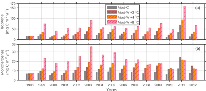
2012, the modelled annual mean isoprene and monoterpene emissions were 20 and 8 mg C m
−2yr
−1, with an increase by 55 and 57 % for 2
◦C summertime warming, respectively.
Warming by 4 and 8
◦C for the same period further elevated isoprene emission for all years, but the impacts on monoter- pene emissions levelled off during the last few years.
At hour-day scale, the WRs seem to be strongly impacted by canopy air T , while at the day–year scale, the WRs are a combined effect of plant functional type (PFT) dynamics and instantaneous BVOC responses to warming. The iden- tified challenges in estimating Arctic BVOC emissions are (1) correct leaf T estimation, (2) PFT parameterization ac- counting for plant emission features as well as physiological responses to warming, and (3) representation of long-term vegetation changes in the past and the future.
1 Introduction
Biogenic volatile organic compounds (BVOCs) are reactive
hydrocarbons mainly emitted by plants. Emissions of these
secondary metabolites are involved in plant growth, plant
defence against biotic and abiotic stresses, plant commu-
nication, and reproduction (Laothawornkitkul et al., 2009;
Peñuelas and Staudt, 2010; Possell and Loreto, 2013). BVOC synthesis is regulated by enzyme activity, and many com- pounds are emitted in a temperature-dependent (T ) and light- dependent (Q) manner (Li and Sharkey, 2013). BVOCs released into the atmosphere react with hydroxyl radicals (OH), which could reduce the atmospheric oxidative capac- ity and therefore lengthen the lifetime of methane (CH
4), as a potent greenhouse gas (Di Carlo et al., 2004; Peñuelas and Staudt, 2010). An increase in BVOC emissions could also el- evate the tropospheric ozone (O
3) concentration when the ra- tio of BVOCs to NO
x(BVOCs / NO
x) is high (Hauglustaine et al., 2005), and increase secondary organic aerosol (SOA) formation (Paasonen et al., 2013). BVOCs could also limit ozone formation when the BVOCs / NO
xratio is low, a situ- ation in which NO
xcan react with O
3(Pusede and Cohen, 2012). Global estimates of non-methane BVOC emissions are in the range of 700–1000 Tg C yr
−1, of which isoprene and monoterpenes contribute most of the emissions (∼ 70 and 11 %, respectively; Sindelarova et al., 2014). The mod- elled emission rates for isoprene are of similar magnitude as for CH
4(Arneth et al., 2008). However, the current esti- mates of regional emission distributions are highly uncertain for both isoprene and monoterpenes for two reasons: (1) the current emission estimates are based on field studies mainly covering tropical, temperate and boreal ecosystems (Guen- ther et al., 2006), lacking observational data for the subarctic and Arctic, and (2) the uncertainties in driving variables (veg- etation distribution and seasonality, climate and environmen- tal data, including soil water availability and the spectrum of the incoming light, abiotic and biotic stress) and in emission responses to these drivers (Guenther et al., 2006; Arneth et al., 2008). For instance, plants adapted to the cold environ- ment of the Arctic appear to respond to warming differently than plants from low latitudes (Rinnan et al., 2014). Until now, the emissions from high latitudes (including the Arc- tic and the subarctic) have been assumed to be minimal due to low foliar coverage, T and plant productivity (Guenther et al., 2006; Sindelarova et al., 2014). However, recent observa- tions from the Arctic have indicated the need for revising the current assumption, as higher emissions from both plants and soils than anticipated in large-scale models have been mea- sured (Ekberg et al., 2009; Holst et al., 2010; Potosnak et al., 2013; Rinnan et al., 2014; Schollert et al., 2014; Kramshøj et al., 2016). Furthermore, field experiments focusing on the effects of climate warming on BVOC emissions have found unexpectedly high responses of BVOC release to a few de- grees of warming (Tiiva et al., 2008; Faubert et al., 2010;
Valolahti et al., 2015; Kramshøj et al., 2016; Lindwall et al., 2016), which has underlined the potentially significant role of Arctic BVOC emissions under changing climate. The Arc- tic is warming at approximately twice the global rate (IPCC, 2013) and the warming-induced drastic vegetation changes (AMAP, 2012) could impose substantial changes in BVOC emissions.
Both isoprene and monoterpenes are produced through the 2-C-methyl-D-erythritol4-phosphate/1-deoxy-D-xylulose-5- phosphate (MEP-DOXP) pathway and are reaction products of their chief precursors, glyceraldehyde-3-phosphate (G3P) and pyruvate. G3P is produced along the chloroplastic Calvin cycle. Mechanistic models have often linked the biosynthesis of isoprene and monoterpenes with photo- synthesis processes (Niinemets et al., 1999; Martin et al., 2000; Zimmer et al., 2003; Grote et al., 2014). In the short term (hours–days), the responses to Q and T of isoprene and monoterpene production are very similar to those of photosynthesis, but with a higher T optimum for BVOC production than photosynthesis (Guenther et al., 1995;
Arneth et al., 2007). Furthermore, some monoterpenes can be emitted from storage pools in plant organs, e.g. glands or resin ducts (Franceschi et al., 2005). Along with the short-term responses, the long-term (days or longer) BVOC dynamics are affected by vegetation composition changes (Faubert et al., 2011; Valolahti et al., 2015), vegetation phenology (Staudt et al., 2000; Hakola et al., 2006), past weather conditions (Ekberg et al., 2009; Guenther et al., 2012) and growing conditions, e.g. soil water and nutrient availability (Possell and Loreto, 2013), atmospheric CO
2(Wilkinson et al., 2009) and ozone levels (Loreto et al., 2004; Calfapietra et al., 2007). Here, we use a process- based ecosystem model to represent BVOC synthesis and emissions. The model simulates vegetation composition dynamically and represents long-term growing environment effects, and thus it is useful in terms of predicting long-term emission responses to environmental changes.
Usually, estimates of BVOC responses to Q and T are based on the Guenther algorithm (referred to here as G93:
Guenther et al., 1993) and observed emission rates are of- ten standardized to emission capacity at standard conditions (T of 30
◦C and photosynthetically active radiation (PAR) of 1000 µmol m
−2s
−1) using the G93 algorithm to allow for comparison with other observations. Potosnak et al. (2013) fitted leaf-level isoprene emission rates to T and Q in moist acidic tundra and found that the G93 algorithm character- ized emissions well with the T response, but not Q response.
However, Ekberg et al. (2009) found that the T response of
the G93 algorithm is not sensitive enough to capture the ob-
served high T responses of wet tundra sedges, which was fur-
ther supported by other studies in the high latitudes (Faubert
et al., 2010; Holst et al., 2010). Furthermore, species-specific
emission profiles (Rinnan et al., 2011, 2014; Schollert et al.,
2015; Vedel-Petersen et al., 2015) have not yet been inte-
grated into the modelling of Arctic BVOC emissions (Ar-
neth et al., 2011; Guenther et al., 2012; Sindelarova et al.,
2014). These need to be included as a trait of plant func-
tional types (PFTs), especially when studying the drastic im-
pacts of climate change on vegetation composition as well
as BVOC emissions in the Arctic. In addition, tundra plants
with relatively dark surfaces and low growth forms (com-
monly less than 5 cm tall) may experience much higher leaf
T than the air T at 2 m height provided by weather stations (Körner, 2003; Scherrer and Körner, 2010; Lindwall et al., 2016), which could lead to larger emissions than anticipated in current models.
The aim of this work was to integrate the observed emis- sion features of Arctic plants into a process-based ecosys- tem model in order to improve the current model estima- tions of Arctic BVOC emissions and to advance our under- standing regarding emission dynamics for Arctic ecosystems in a warming future. The process-based dynamic ecosystem model LPJ-GUESS (Lund–Potsdam–Jena General Ecosys- tem Simulator) (Smith et al., 2001, 2014) was used as a platform to simulate short-term and long-term responses of BVOC emissions to changes in climate for Arctic plants. The model links isoprene and monoterpene production with pho- tosynthesis (Arneth et al., 2007; Schurgers et al., 2009). For the application to a subarctic heath tundra, the process pa- rameterization utilized field observations of long-term (13- year) warming treatment effects on vegetation composition and BVOC emissions (Tiiva et al., 2008; Faubert et al., 2010;
Valolahti et al., 2015). The specific objectives of this study were (1) to capture the observed T response of BVOC emis- sions for a subarctic ecosystem, (2) to address the importance of short-term and long-term impacts of warming on ecosys- tem as well as BVOC emissions, and (3) to diagnose key model developments needed to better present BVOC dynam- ics for the Arctic region.
2 Materials and methods
2.1 Study area and observational data
The data used in this modelling study were collected at a dwarf shrub/graminoid heath tundra located in Abisko, northern Sweden (68
◦21
0N, 18
◦49
0E). The vegetation con- sists of a mixture of evergreen and deciduous dwarf shrubs, graminoids and forbs. A long-term field experiment was es- tablished at this site in 1999 to investigate the effects of cli- mate warming and increasing litter fall, resulting from the ex- panding tundra vegetation, on the functioning of the ecosys- tem. The experiment included control (C), warming (W), lit- ter addition (L) and combined warming and litter addition (WL) treatments (Rinnan et al., 2008). In the current study, we only focused on the observations from the C and W treat- ments. Each treatment, covering an area of 120 × 120 cm, was replicated in six blocks. The W treatments used open- top chambers (OTCs), which passively increased air T by around 2
◦C and also caused around 10 % reduction in PAR (Valolahti et al., 2015).
During the years 2006, 2007 and 2012, BVOC emission rates were measured for all plots by sampling air from trans- parent polycarbonate chambers into adsorbent cartridges us- ing a push–pull enclosure technique and analysis by gas chromatography–mass spectrometry. The enclosure covered
a 20 cm × 20 cm area in each plot. The air T inside the en- closure and PAR in ambient conditions were measured dur- ing the sampling. For 2006–2007, the datasets for isoprene emission can be found in Tiiva et al. (2008) and those for monoterpenes in Faubert et al. (2010). For the year 2012, isoprene and monoterpene emissions have been published by Valolahti et al. (2015). Notably, BVOCs in this study only refers to isoprene and monoterpenes. Closed chamber-based CO
2fluxes were measured in the same area for 2006, 2007, 2010 and 2012 (data from 2006 and 2007 were published in Tiiva et al., 2008, whilst data from 2010 and 2012 have not been published before). Species composition and cover- age in the plots in the same years were estimated by point- intercept-based method, in which a hit is recorded each time a plant species is touched by a pin lowered through 100 holes covering the plot area of 20 cm × 20 cm (Tiiva et al., 2008;
Valolahti et al., 2015). Species composition was measured in June for 2006, 2010 and 2012, and in June, July and August for the year 2007.
2.2 LPJ-GUESS
2.2.1 LPJ-GUESS general framework
LPJ-GUESS is a climate-driven dynamic ecosystem model with mechanistic representations of plant establishment, mortality, disturbance and growth as well as soil biogeo- chemical processes (Smith et al., 2001; Sitch et al., 2003).
Vegetation in the model is defined and grouped by PFTs, which are based on plant phenological and physiognomic features, combined with bioclimatic limits (Sitch et al., 2003;
Wolf et al., 2008). The model has been widely and success- fully applied for simulating vegetation and soil carbon fluxes as well as vegetation dynamics at different spatial scales (Wolf et al., 2008; Hickler et al., 2012; Smith et al., 2014;
Tang et al., 2015). In the model, individuals of each PFT in the same patch (replicate unit in the model, representative of vegetation stands with different histories of disturbance and succession) can compete for light and soil resources.
Plant establishment and mortality are represented as stochas- tic processes, but influenced by life history, resource sta- tus and demography (Smith et al., 2014). For summergreen plants, an explicit phenological cycle is implemented, which is based on the accumulated growing degree-day (GDD) sum for leaf onset and full leaf cover.
In LPJ-GUESS, a generalized Farquhar photosynthesis
model (Farquhar et al., 1980; Collatz et al., 1991) for large-
scale modelling is used to simulate canopy-level carbon as-
similation and the generalized model is built on the assump-
tion of optimal nitrogen (N) allocation in the vegetation
canopy (Haxeltine and Prentice, 1996a, b). Daily net photo-
synthesis is estimated using a standard non-rectangular hy-
perbola formulation, which gives a gradual transition be-
tween the PAR-limited (J
E) and the rubisco-limited (J
C)
rates of assimilation (Haxeltine and Prentice, 1996b). For C
3plants, J
Eis a function of the canopy-absorbed PAR, the in- trinsic quantum efficiency for CO
2uptake (α
c3), the CO
2compensation point (0
∗) and the internal partial pressure of CO
2(p
i) (Collatz et al., 1991; Haxeltine and Prentice, 1996b). J
Cis related to the maximum catalytic capacity of rubisco per unit leaf area (V
m), 0
∗, p
iand the Michaelis–
Menten constant for CO
2and O
2. Stomatal conductance in- fluences the intercellular CO
2, p
iand canopy transpiration.
2.2.2 BVOC modelling
In LPJ-GUESS, isoprene (Arneth et al., 2007) and monoter- pene (Schurgers et al., 2009) emissions are simulated as a function of the photosynthetic electron flux. The productions of isoprene (E
I) and monoterpenes (E
M) are computed as E = α J ε, where α = p
i− 0
∗6 × (4.67p
i+ 9.330
∗) , (1) where J is the rate of photosynthetic electron transport and α converts photon fluxes into terpenoid units. The synthesis of both compounds is linked to J (Niinemets et al., 1999, 2002) and a fraction (ε) of the electron transport contributing to terpenoid production (Eq. 2) is determined from a plant- specific fraction under standard conditions (ε
S, usually at a T of 30
◦C and a PAR of 1000 µmol m
−2s
−1) which is adjusted for leaf T , seasonality (σ ), and atmospheric CO
2concentra- tion:
ε = f (T )f (σ )f (CO
2)ε
S. (2) The standard fraction ε
Sis computed from the often reported standard emission rate (emission capacity) together with the simultaneously estimated photosynthetic electron flux under these standard conditions (standard T and PAR) in the model.
The choice of different T and PAR as standard conditions will influence the value for ε
Sand thus the estimated emis- sion rate under different conditions. The T response corrects for the T optimum for terpenoid synthesis, which is higher than that for photosynthesis:
f (T ) = e
ατ(T−TS). (3) The parameter α
τrepresents the T sensitivity and the stan- dard temperature (T
S) is often 30
◦C (adjusted to 20
◦C in this study). In the model, daily mean T (T
d, model input) has been adjusted to daylight hours T based on day length as well as daily T range (Arneth et al., 2007) and the daytime T is used for calculating daily emission rates. For the study in the subarctic, the often-used reference T
Sof 30
◦C and the T responses (α
τ) were adjusted based on the observation data and will be discussed below. The seasonality function, f (σ ), was applied to both isoprene and monoterpene pro- duction and is based on a degree-day sum in spring and day- length thresholds in autumn (Arneth et al., 2007; Schurgers et al., 2009). The atmospheric CO
2concentration enhances ter- penoid synthesis when the concentration is lower than am- bient, and vice versa, which is represented by the function
f (CO
2) (Arneth et al., 2007). The model assumes that both isoprene and monoterpenes are produced in the same path- way and that they respond to CO
2concentration in the same way.
For monoterpenes, a storage pool (m) is assigned to repre- sent the specific (long-term) storage of monoterpenes within a leaf (Schurgers et al., 2009). The storage pool is only im- plemented for coniferous and herbaceous PFTs (see Table S1 in the Supplement). The emission of monoterpenes from the storage (E
Ms) is a function of T
dand m with an average res- idence time (τ ). τ
Sis the residence time at the standard T of 30
◦C (adjusted to 20
◦C in this study, consistent with the modification on the T responses of terpenoid synthesis). The residence time τ is adjusted based on the standard condition τ
Sfor T
dresponses with a Q
10relationship.
E
Ms= m/τ
τ = τ
SQ
(T10d−TS)/10(4)
In LPJ-GUESS, the BVOC response to light resides in the photosynthesis processes (light dependence of J in Eq. 1).
Additionally, considering the high sensitivity of BVOC pro- duction to leaf T , the model applies a computation of leaf T based on air T and energy balance constraints (Arneth et al., 2007; Schurgers et al., 2009). The calculation of leaf T in the model was based on solving the leaf energy balance, where the incoming shortwave and longwave radiation are balanced by the outgoing longwave radiation and sensible heat fluxes as well as latent heat loss. The existing leaf energy balance equations appeared to underestimate the incoming longwave radiation under overcast conditions, which has been updated by specifically considering the cloud emission of longwave radiation relative to clear-sky condition (Sedlar and Hock, 2009). The estimated leaf T , rather than air T , was used for both photosynthesis and BVOC synthesis. Water loss (latent heat fluxes) is regulated by stomatal conductance and soil water content, which is also linked to leaf T estimation in the model.
2.3 Simulation setup 2.3.1 Input data
The daily climate data of air T , air T range and precip- itation for the period 1984–2012 (Callaghan et al., 2013;
Tang et al., 2014) were provided by the Abisko scien-
tific research station (Abisko Naturvetenskapliga Station,
ANS). Four gaps in daily radiation data from ANS (during
the periods of 1 January–30 June 1984, 9–16 June 2016,
13–15 February 2007, 23 July–17 August 2011) were
filled with the Princeton reanalysis dataset (Sheffield et
al., 2006) for the grid cell nearest Abisko. The annual
CO
2concentrations for the whole study period (1984–2012)
were obtained from McGuire et al. (2001) and TRENDS
(http://cdiac.esd.ornl.gov/). The air T inside the enclosure
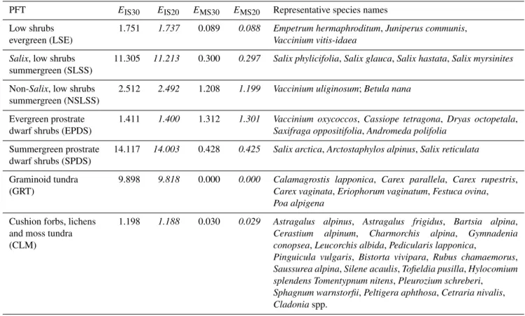
Table 1.
Plant functional types (PFTs) and representative species in the study area. The emission capacity of isoprene (E
IS, µg C g dw
−1h
−1)and monoterpenes (E
MS, µg C g dw
−1h
−1)at 20
◦C (in italics) used the adjusted temperature response curve from this study, whilst the averaged literature values of the emission capacity at 30
◦C were based on the Guenther’s algorithms. The values are based on the available growing season leaf-level measurements from the Arctic.
PFT
EIS30 EIS20 EMS30 EMS20Representative species names Low shrubs
evergreen (LSE)
1.751 1.737 0.089 0.088 Empetrum hermaphroditum, Juniperus communis, Vaccinium vitis-idaea
Salix, low shrubs summergreen (SLSS)
11.305 11.213 0.300 0.297 Salix phylicifolia, Salix glauca, Salix hastata, Salix myrsinites Non-Salix, low shrubs
summergreen (NSLSS)
2.512 2.492 1.208 1.199 Vaccinium uliginosum; Betula nana Evergreen prostrate
dwarf shrubs (EPDS)
1.411 1.400 1.312 1.301 Vaccinium oxycoccos, Cassiope tetragona, Dryas octopetala, Saxifraga oppositifolia, Andromeda polifolia
Summergreen prostrate dwarf shrubs (SPDS)
14.117 14.003 0.428 0.425 Salix arctica, Arctostaphylos alpinus, Salix reticulata Graminoid tundra
(GRT)
9.898 9.818 0.000 0.000 Calamagrostis lapponica, Carex parallela, Carex rupestris, Carex vaginata, Eriophorum vaginatum, Festuca ovina, Poa alpigena
Cushion forbs, lichens and moss tundra (CLM)
1.198 1.188 0.030 0.029 Astragalus alpinus, Astragalus frigidus, Bartsia alpina, Cerastium alpinum, Charmorchis alpina, Gymnadenia conopsea, Leucorchis albida, Pedicularis lapponica,
Pinguicula vulgaris, Bistorta vivipara, Rubus chamaemorus, Saussurea alpina, Silene acaulis, Tofieldia pusilla, Hylocomium splendens Tomentypnum nitens, Pleurozium schreberi, Sphagnum warnstorfii, Peltigera aphthosa, Cetraria nivalis, Cladonia spp.
and ambient PAR at canopy level were also used as the model inputs for each measuring day (Tiiva et al., 2008; Faubert et al., 2010; Valolahti et al., 2015).
2.3.2 Plant functional types
The dominant plant species from the observations (Valolahti et al., 2015) were divided into seven PFTs (Table 1). The PFT parameters (see Table S1) were mainly derived from previ- ous studies for the Arctic region using LPJ-GUESS (Wolf et al., 2008; Miller and Smith, 2012; Tang et al., 2015), but the Arctic PFT lists were extended to consider BVOC emission characteristics. The low summergreen shrubs (LSS) were divided into a Salix type (SLSS; high isoprene emitter) and a non-Salix type (NSLSS; e.g. Betula nana dominance, predominantly monoterpenes rather than isoprene emitters) (Schollert et al., 2014; Vedel-Petersen et al., 2015). Fur- thermore, due to the abundance of prostrate dwarf shrubs (PDS) in the study area, distinguishing PDS (canopy height lower than 20 cm) from low shrubs (canopy height lower than 50 cm) was implemented through adjusting parameters controlling vegetation height. The PDS type was further di- vided into two PFTs with evergreen and deciduous phenol- ogy. Moss, widely appearing in the study area, was not dis-
tinguished from forbs and lichens, due to limited data for pa- rameterizing moss physiognomic features and their prefer- able growing conditions.
In LPJ-GUESS, the crown of each tree is divided into thin
layers (original value is 1.0 m in a forest canopy) in order to
integrate PAR received by each tree. The thickness of this
layer was reduced to 10 cm in this study to better capture
the vertical profile of low and prostrate shrubs. In addition,
the original specific leaf area (SLA, m
2kg C
−1) values in
LPJ-GUESS were estimated based on a fixed dependency on
leaf longevity (Reich et al., 1997). In our study, a fixed SLA
was assigned to each PFT (Oberbauer and Oechel, 1989)
to improve the simulated leaf area index (LAI) for Arctic
plants. Emission capacities for the PFTs were determined
from available leaf-level measurement data from the subarc-
tic and Arctic. The details about the data sources for parame-
terizing emission capacity at 30
◦C (E
IS30, E
MS30) and 20
◦C
(E
IS20, E
MS20) can be found in Table S2 and the averaged
emission capacities (among all literature data in Table S2)
for each PFT as well as the representative plant species can
be found in Table 1. The emission rates from the literature
are generally provided as standardized emission capacities at
30
◦C using the G93 algorithm, and these values were further
Figure 1.
The observed isoprene emission rates in relation to the chamber air temperature in July over three field seasons (2006, 2007, 2012) in the Abisko tundra heath.
rescaled to 20
◦C using the adjusted T response curve from this study (Fig. 1).
2.3.3 Model calibration and evaluation
The modelled CO
2fluxes, LAI and BVOC T response were first calibrated before evaluating the modelled daily BVOC emission rates. Two out of four years’ (2006 and 2007) mea- sured net ecosystem production (NEP), ecosystem respira- tion (ER) and estimated gross primary production (GPP) as well as point-intercept-based species composition were used for calibrating. The data for the other 2 years (2010 and 2012) were used for evaluating the simulated carbon cy- cle processes. Previous studies focusing on light responses of NEP for Arctic plants (Shaver et al., 2013; Mbufong et al., 2014) have reported relatively low quantum efficiencies (α
c3) caused by overall low sun angle conditions and low leaf area. A thorough sensitivity study of parameters used in LPJ-GUESS (Pappas et al., 2013) has found that α
c3is the most influential parameter in terms of the simulated vege- tation carbon fluxes. Also, a pre-evaluation of the modelled CO
2fluxes with the observations in this study using the de- fault α
c3value (0.08) has found a large overestimation of both GPP and ER (not shown). Therefore, a sampling of α
c3(using the range of 0.02 to 0.125 µmol CO
2µmol photons
−1, proposed by Pappas et al., 2013) was conducted to find the best value to depict the observed GPP, ER and LAI of the years 2006 and 2007 for the subarctic ecosystem (Fig. S1 in the Supplement). After calibration, the model was evaluated with the simulated CO
2fluxes and vegetation composition using the observed CO
2fluxes and the point-intercept-based plant coverage data from 2010 and 2012, respectively.
The daytime air T in the study area is often below 20
◦C
(Ekberg et al., 2009), and standardization of terpenoid emis-
sions to 20
◦C, instead of 30
◦C, has been suggested for mod-
elling in boreal and Arctic ecosystems (Holst et al., 2011,
Ekberg et al., 2009) due to plant adaptation to low T en-
vironment. In the model, the photosynthetic electron fluxes
under standardized conditions are simulated in order to con-
vert the input emission capacity to the standard fraction (ε
S,
see Eq. 2). The choice of the standardized T (used in Eq. 3
as well as in estimating photosynthesis rates at this T ) will
influence the estimated fraction of electron fluxes for BVOC
synthesis. In this study, data fitting to the suggested standard
T of 20
◦C was conducted using the observed ecosystem-
level isoprene emission rates in July together with measure-
ment chamber air T from the C plots. The observations were
mostly conducted during daytime with relatively high PAR
values, and therefore the response of the emission rates to
light was not specifically considered in the current data fit-
ting. Potential feedbacks from the variations in the atmo-
spheric CO
2concentration were ignored for the 3 years with
isoprene sampling (a rough model estimation of ∼ 3% re-
duction in emissions between 2006 and 2012). The data col-
lected from different blocks were separated for the curve fit-
ting and the parameters controlling T response (α
τin Eq. 3)
were determined (Fig. 1). An adjusted α
τvalue of 0.23 was
chosen after fitting all the data from July over 3 years’ mea-
surements. Apart from the low R
2value for block 1, the data
were well captured by the exponential shape (R
2≥ 0.8) of
the T response curve. The calibrated T responses were used
for standardizing leaf-level emission rates (see M
IS20and
E
MS20, Table 1) as well as estimating emission rates in the
model. This adjusted T response was also evaluated with the
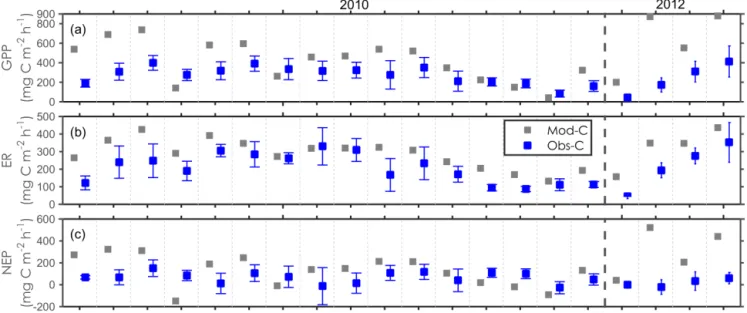
Figure 2.
Modelled (grey) and observed (blue) gross primary production (GPP,
a), ecosystem respiration (ER,b), and net ecosystem pro-duction (NEP,
c) for the growing season of 2010 and 2012 in the control plots at the Abisko tundra heath. Error bars indicate the standarddeviation for the six replicates.
observed enclosure air T and monoterpene emission rates in July (R
2= 0.66 for all blocks).
The abundance of each PFT was evaluated using simulated LAI against the point-intercept-based vegetation composi- tion. The species were grouped into the corresponding PFTs for comparison and the point-intercept-based hits within the same PFT group were summed. The summed hits were di- vided by 100 pin hits to compare with the modelled LAI. The point-intercept-based species abundances and LAI are not comparable one to one throughout growing seasons, since the measurement could include pin hits on different plant parts, whereas LAI only explains leaf coverage. However, the point-intercept-based coverage approaches leaf coverage when the deciduous leaves become fully developed during the growing season.
After calibration of the modelled CO
2fluxes and LAI, the modelled isoprene and monoterpene emission rates were compared with the observations. The simulated daytime av- erage emissions (µg C m
−2h
−1, daytime emission rates di- vided by day length) do not allow an accurate comparison with the observed emission rates, which were typically ob- tained in the middle of the day (between 09:00 and 17:00).
Therefore, an additional estimate of the emission rates for the conditions prevailing during the sampling was made. This was done by computing the emission applying the measured air T inside the enclosure and PAR during the sampling time for photosynthesis and BVOC emissions. This computation was performed twice: once using the original T response (α
τ= 0.1, T
S= 30
◦C, E
IS30and E
MS30, Eq. 3) and once
with the adjusted T response (α
τ= 0.23, T
S= 20
◦C, E
IS20and E
MS20, Eq. 3 and Fig. 1).
The model’s performance in modelling BVOC emissions was evaluated by Willmott’s index of agreement (A) (Eq. 5) and mean bias error (B) (Eq. 6). The index A describes the agreement between the modelled fluxes (E
i) with the ob- served (O
i) and a value close to 1 indicates a good agree- ment. The index B estimates the mean deviation between the modelled and observed values (Willmott et al., 1985) and val- ues close to 0 indicates models’ good agreement with obser- vations.
A = 1 −
N
P
i=1
| E
i− O
i|
N
P
i=1
( E
i− O
+
O
i− O )
(5)
B =
N
P
i=1
(E
i− O
i)
N , (6)
where O is the observed mean value and N is total number of data records.
2.3.4 Effect of warming
To simulate the observed warming responses from the OTCs, a warming of 2
◦C was imposed in the model for the growing season (the period with OTC warming) (Tiiva et al., 2008;
Valolahti et al., 2015). The modelled warming responses
(WRs, difference between C and W treatments) using the
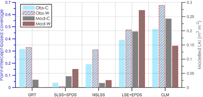
Figure 3.
Point-intercept-based vegetation coverage and modelled leaf area index (LAI, m
2m
−2) averaged for the growing season 2010 and 2012 for the control (C) and warming (W) treatments in the Abisko tundra heath. Different
yaxes are used for the observed (Obs) and the modelled (Mod) coverage to allow comparison of warming effects. GRT: graminoid tundra; SLSS: Salix, low shrubs summergreen; SPDS:
summergreen prostrate dwarf shrubs; NSLSS: non-Salix, low shrubs summergreen; LSE: low shrubs evergreen; EPDS: evergreen prostrate dwarf shrubs; CLM: cushion forbs, lichens and moss tundra.
original T response and the adjusted T response were com- pared with the observed WRs. Furthermore, additional simu- lations with a warming by 4 and 8
◦C, reflecting the range of climatic projections in this region (IPCC, 2013), were also conducted to test for the anticipated ecosystem-scale re- sponses to different levels of warming.
3 Results
3.1 Modelled CO
2fluxes and vegetation composition The simulated ecosystem CO
2fluxes and LAI were sen- sitive to the parameter value chosen for α
c3, which describes the efficiency in converting solar radiation to carbohydrates, and which was varied between 0.02 and 0.125 µmol CO
2µmol photons
−1following Pappas et al. (2013) (Fig. S1). For CO
2fluxes, the lowest root- mean-square error (RMSE) values occurred at 0.035 µmol CO
2µmol photons
−1for GPP and ER, while the lowest RMSE value for LAI was 0.051 µmol CO
2µmol photons
−1when comparing with the observations for 2006 and 2007.
A value of 0.040, consistent with the study by Shaver et al. (2013), was selected for α
c3to limit the RMSE values of the modelled CO
2fluxes and LAI. Using this value for α
c3, the model captured the observed day-to-day variations as well as the magnitude of the chamber-based GPP, ER and NEP for 2010 and 2012, with an overestimation of CO
2fluxes (particularly for the early growing seasons, Fig. 2) and a large underestimation of LAI (Fig. 3). For the year 2012, the model showed large overestimations of the observed GPP
and ER for the limited number of measurements in this grow- ing season.
For the five PFT groups, the modelled growing season LAI values for 2010 and 2012 were much lower than the point- intercept-based coverage estimations from the field observa- tions (note different left and right axis scales in Fig. 3 to al- low comparison of relative changes in response to warming), except for the Salix-type summergreen shrubs and decidu- ous prostrate dwarf shrubs (SLSS + SPDS). The dominance of two vegetation groups in the C plots – forbs/lichens and evergreen shrubs – was consistent between the modelled and the observed.
In response to 2
◦C warming, the modelled LAI for the shrub PFTs (SLSS + SPDS, NSLSS, LSE + EPDS) showed an increase, while the modelled LAI for graminoids and forbs/lichens largely decreased (Fig. 3). For the two groups of shrubs (NSLSS and LSE + EPDS), the modelled increase is in agreement with the observations. However, the observed large increase in the coverage of forbs/lichens and a de- creased coverage of graminoids in the W treatments for the year 2010 and 2012 were not captured by the model.
3.2 Modelled BVOC emissions
BVOC emissions are closely linked to leaf as well as ecosys-
tem development. Simulating seasonal variation in leaf area
and vegetation composition enables us to assess the model
performance in representing short-term emission changes in
response to T and PAR, as well as long-term changes in veg-
etation development and distribution. The seasonal variations
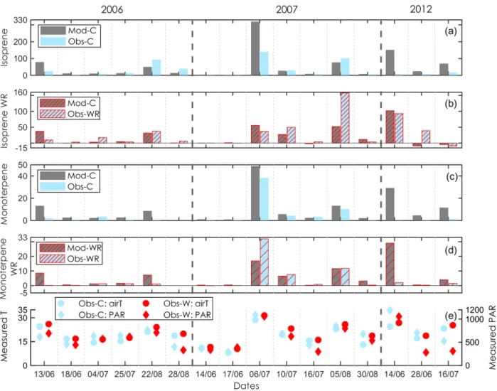
Figure 4.
Comparison of the modelled
(a)isoprene and
(c)monoterpene emission rates with the observations in the control (C) plots and evaluation of modelled warming responses (WRs) with the observed WRs
(b, d)at the Abisko tundra heath. The observed enclosure air temperature (air
T) and PAR outside the enclosure are displayed in
(e). Mod: modelled; Obs: observed.in the modelled daily BVOC emissions as well as the span of all BVOC samplings over 3 years are presented in Fig. S2.
3.2.1 Daily emissions
Emission rates in the control (ambient) conditions The observed air T and PAR showed day-to-day varia- tions through the sampling periods (Fig. 4e), which re- sulted in strong daily variations in the observed BVOC emis- sions (Fig. 4a and c). These observed variations in isoprene and monoterpene emissions were generally captured by the model for 2006 and 2007. For the year 2012, the model over- estimated both isoprene and monoterpene emission rates over the three sampling days. Noticeably, the model used air T at 2 m height from the ANS station to extrapolate the leaf T for estimating daily BVOC emissions (Fig. S2), while the ob- served air T and PAR during the sampling hours were used for modelling the emissions to directly compare with the ob- served (Fig. 4). The modelled high emission rates for a few
days (e.g. 10 July 2007, 14 June 2012) were directly linked to the observed high T and PAR at the canopy level (Fig. 4e).
Averaged over all measuring days in 2006 and 2007, the modelled and observed isoprene emission rates were 46.6 and 34.7 µg C m
−2h
−1, and the modelled and observed monoterpene emission rates were 8.5 and 5.3 µg C m
−2h
−1, respectively. For the year 2012, the modelled emission rates (80.4 and 14.9 µg C m
−2h
−1for isoprene and monoterpenes, respectively) were much higher than the observed (9.1 and 0.5 µg C m
−2h
−1, for isoprene and monoterpenes, respec- tively). The large overestimation by the model in the year 2012 was also seen for GPP and ER (Fig. 2).
Emission responses to 2
◦C warming
In response to warming by the OTCs, the observed enclo-
sure air T in the W plots was 2.1
◦C higher than that in
the C plots averaged over the three growing seasons with ob-
servations. For isoprene, the observed magnitudes of WRs
(Fig. 4b) were captured reasonably well by the model, ex-
Figure 5.
Scatter plot of the modelled (Mod.) and the observed (Obs.) warming responses (WRs) for both isoprene
(a)and monoterpene
(b),using the adjusted (Adj) and the original
T(Orig) response.
Figure 6.