Optical method for measuring bed topography and flow depth in an experimental flume

(1)

HAL Id: hal-01499426

https://hal-univ-paris.archives-ouvertes.fr/hal-01499426

Submitted on 31 Mar 2017

HAL is a multi-disciplinary open access

archive for the deposit and dissemination of

sci-entific research documents, whether they are

pub-lished or not. The documents may come from

teaching and research institutions in France or

abroad, or from public or private research centers.

L’archive ouverte pluridisciplinaire HAL, est

destinée au dépôt et à la diffusion de documents

scientifiques de niveau recherche, publiés ou non,

émanant des établissements d’enseignement et de

recherche français ou étrangers, des laboratoires

publics ou privés.

depth in an experimental flume

A Limare, M Tal, M Reitz, E Lajeunesse, F Métivier

To cite this version:

A Limare, M Tal, M Reitz, E Lajeunesse, F Métivier. Optical method for measuring bed topography

and flow depth in an experimental flume. Solid Earth, European Geosciences Union, 2011, 2, pp.143

- 154. �10.5194/se-2-143-2011�. �hal-01499426�

(2)

www.solid-earth.net/2/143/2011/ doi:10.5194/se-2-143-2011

Solid Earth

Optical method for measuring bed topography and flow depth in an

experimental flume

A. Limare1, M. Tal1,*, M. D. Reitz2, E. Lajeunesse1, and F. M´etivier1

1_{Equipe de Dynamique des Fluides G´eologiques, Institut de Physique du Globe de Paris (IPGP, UMR 7154, CNRS,}

Univ. Paris Diderot), 1 rue Jussieu, 75238 Paris Cedex 05, France

2_{Department of Physics and Astronomy, University of Pennsylvania, 209 S. 33rd St., Philadelphia, PA 19104, USA}

*_{now at: Univ. Aix-Marseille, CEREGE UMR 6635, Europˆole de l’Arbois, BP 80, 13545 Aix-en-Provence cedex 04, France}

Received: 1 March 2011 – Published in Solid Earth Discuss.: 15 March 2011 Revised: 17 June 2011 – Accepted: 7 July 2011 – Published: 28 July 2011

Abstract. We describe an optical method known as moir´e for

acquiring quasi-simultaneous measurements of bed topogra-phy and flow depth in laboratory experiments. The moir´e method is based on projecting a fringe pattern (grating) on the bed and analyzing the deformation of the pattern caused by the topography with respect to a reference plane. The height of the object is encoded in the phase of the pattern and can be retrieved either through Fourier transform or phase shifting algorithms. The methodology enables image-based non-contact measurements over a continuous surface at very high spatial and temporal resolutions. We use a commercial software package of a moir´e method called Light3D to map bed topography and flow depth in an experimental braided channel and demonstrate how the method can be used to characterize a full range of statistics not previously possible.

1 Introduction

Laboratory experiments are an important tool in the study of morphodynamics and have been used to investigate a wide range of landforms ranging from submarine channels (M´etivier et al., 2005) to the response of drainage basins to tectonic uplift (Lague et al., 2003; Turowski et al., 2006). Analog models offer an opportunity to examine interactions underlying naturally complex systems in a well-controlled environment, and to observe how systems evolve over much longer timescales than possible in the field. In fluvial mor-phodynamics, experiments have been used successfully to

Correspondence to: A. Limare

(limare@ipgp.fr)

reproduce and visualize sediment-flow interactions and bed morphology (Lajeunesse et al., 2010a) and have helped im-prove our understanding of self-formed channels with mo-bile beds and stable banks (Armstrong, 2003; Malverti et al., 2008), braiding kinematics (M´etivier and Meunier, 2003), bedforms (e.g., Coleman and Eling, 2000), seepage chan-nels (Ni and Crave, 2006), alluvial fans (Reitz et al., 2010), knickpoints (Malverti et al., 2007), and alluvial bed mor-phodynamics (Coleman and Eling, 2000; Devauchelle et al., 2010a,b). (For a more complete review, see Lajeunesse et al., 2010b; Paola, 2010).

Several experimental techniques have been developed specifically for data acquisition in experiments with the ob-jective of monitoring both bed topography and flow charac-teristics. Classical approaches to the measurement of bed topography in these types of experiments include moving point or line probes along the experimental surface such as single beam time-of-flight laser profiler mounted on a con-trolled carriage (Lague et al., 2003), or scanning a stripe laser over the experimental surface (Rice et al., 1988; Darboux and Huang, 2003; Huang et al., 2007a). These techniques often require interrupting the experiment (i.e., shutting off the flow) at regular intervals and moving the probe, often very slowly, over the temporarily frozen surface. A faster and continuous alternative is based on monitoring the exper-iment with a camera set to capture time-lapse images of the evolving surfaces. This method allows reconstruction of the topography using stereoscopy (Chandler et al., 2001).

To map flow depths, depth-from-luminosity measurements have been successfully acquired over both fixed and evolving topography. Aureli et al. (2008) mapped the evolving flow depth over a flat, transparent floor, illuminated from below, by adding blue dye to the water and monitoring from above

(3)

the distribution of light attenuation. Tal and Paola (2007) used rhodamine dye to estimate the distribution of water depth in braided and single-thread channels. Both methods involve using flow with a constant dye concentration and cal-ibrating the depth dependence of the luminosity as recorded by camera images. These methods are closely related to the common use of fluorescent dye to monitor groundwater flow patterns (Weiler and Fl¨uhler, 2004; Huang et al., 2007b). While independent methods for measuring bed topogra-phy and flow depth exist, simultaneous measurement of bed topography and flow depth remains a challenge. Huang et al. (2010) proposed a novel combination of methods to study the morphodynamics of sediment beds under the action of flow-ing water. In this method, a laser stripe is scanned back and forth across the experimental surface while a fluorescent dye is mixed with the flowing water, allowing simultaneous map-ping of both bed topography and water depth at millimetric resolution and sub-millimetric accuracy (0.6 mm).

In this paper we describe a method for acquiring quasi-simultaneous measurements of bed topography and flow depth at very high resolution using an optical method known as moir´e. This method requires the interrupting of the flow and the acquisition of two sets of topographies with and with-out flow. We begin by describing the different steps in ap-plying this version of the moir´e method to reconstruct the topography of a dry bed. We then discuss the case of an ex-perimental alluvial plain with water flowing over the bed. Fi-nally, we apply this method to a microscale braided channel experiment and discuss the quality of the results obtained.

The moir´e method has been successfully applied in metrol-ogy studies (Chiang, 1983), industrial inspection (Sansoni et al., 2000), human body mapping for medical diagnosis (Halioua and Liu, 1989; Kozłowski and Serra, 1997) and art inspection (Br´emand et al., 2007).

In geomorphology, simplified versions of the moir´e method have been previously used in laboratory physical ex-periments to study granular flows (Pouliquen and Forterre, 2002), incision dynamics of subaqueous channels (Lancien et al., 2005), and micro-scale braided rivers (Meunier, 2004). In these studies the method was implemented by projecting a single grid onto the evolving surface and analyzing how it is deformed (captured by time-lapse images) using a Fourier transform. This approach has the advantage of being low cost (minimum materials required include only a digital camera and an overhead or slide projector) and is relatively simple to implement. However, it offers limited resolution and a lim-ited field of view, and therefore limlim-ited object dimensions.

Here we present a more elaborate implementation of the moir´e method to two fluvial geomorphology studies. This method was developed at the Laboratory of Solid State Me-chanics of the University of Poitiers, France (Breque et al., 2004). This commercial software was already used for the experimental investigation of bedforms dynamics in a config-uration where the sediment supply was limited (Dreano et al., 2010). It uses a phase shifting method for phase calculation,

robust phase unwrapping combined with gray coding and a calibration procedure that allows assessing the geometric pa-rameters. The method proves relatively easy to use and to calibrate. The number of projected images can be varied so one can switch between high resolution and fast acquisition time according to the requirements of the experiments.

Braiding has always been easy to reproduce in the lab and many experiments have been developed since the fifties (Ashmore, 1982; Federici and Paola, 2003; Schumm, 1977; Schumm et al., 1987). Yet the existence of multiple highly dynamic threads poses challenging issues. The technique we present here enables us to address two key issues in braided river studies: topographic evolution of the bed and shear stress distribution.

The novelty here is that we are able to get the instanta-neous depth everywhere on the braid plane. Thus, for the first time, we are able to compute PDFs of flow depth and probably shear stress distributions. To our knowledge there exist only two published PDFs for natural braided streams (Paola, 1996; M´etivier et al., 2011) and one for experimental braided rivers (Tal and Paola, 2007). Both of these records are rough and limited, precisely because of the acquisition techniques. Yet these studies and both theoretical and nu-merical considerations (Paola, 1996, 2001) clearly point to the key importance of such measurements in order to under-stand the physics of sediment transport in a braided river.

2 Presentation of the moir´e method

2.1 General considerations

The moiré phenomenon can be observed when superimpos-ing two (or more) periodic or quasiperiodic structures; the so-called moiré method is not in fact one method, but rather a group of methods. Depending upon how or from what type of geometric patterns the moiré fringes are created, they as-sume different physical signification. The method of moiré contouring is a well known technique for 3-D shape measure-ment (Patorski, 1993): the moiré fringes are created by the superposition of two periodic alternating line-space patterns, i.e., linear gratings. One of these gratings is to be distorted by an object whose deformation or shape is represented by the moiré fringes. The main merits of the moiré topography are:

1. Measurements are whole-field, an advantage over point-by-point or line methods.

2. Data acquisition and processing is relatively fast so in-vestigations can be done in quasi real-time and the pro-cess automated.

(4)

4. Differential as well as absolute measurements are possi-ble so that the influence of system geometry and optical aberrations may be removed.

The output of a moir´e fringe technique is a fringe pattern which must be analysed so that the results can be presented in a numerical or graphical form. In the process of fringe pattern analysis, the only measurable quantity is the intensity that has a cosinusoidal profile:

I (x,y) = a(x,y) + b(x,y)cos[φ (x,y)] (1) where I (x,y) is the measured intensity, φ (x,y) is the phase of the signal, a(x,y) is the background intensity and b(x,y) is the local contrast; both a(x,y) and b(x,y) being propor-tional to the surface reflectivity. The phase φ (x,y) contains the desired out-of-plane information and should be extracted from Eq. (1). The main problems related to the phase evalu-ation are:

1. The phase is screened by two other functions: the back-ground intensity a(x,y) and the local contrast b(x,y). 2. Due to the periodicity of cosinusoidal intensity profile,

the phase is only determined modulo 2π .

3. Due to the even character of the cosine function, the sign of φ(x,y) cannot be extracted from a single measure-ment, so that one cannot distinguish between depression and elevation without a priori knowledge.

If the moir´e method usually supposes the superposition of two or more periodic structures, in this work we used a co-sine fringe pattern projection. Simple Fourier analysis of the fringe pattern in the presence of the spatial carrier frequency, for example in the x direction, gives:

φ0(x,y) =2πf0x + φ (x,y) (2)

The phase to be measured, φ(x,y), modulates the carrier fringe pattern and this modulation is indicated by changes in the position and spatial frequency of the fringes.

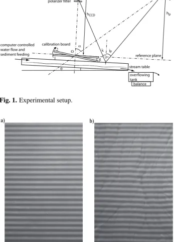
Experimentally, the method consists of projecting a grat-ing of parallel lines onto an object, in our case a stream table (Fig. 1). The topography of the object will deform the grating (Fig. 2b) and this deformation is calculated with respect to a reference plane which in our case is a flat bed (Fig. 2a). The height of the object is encoded in the phase of the pattern and can be retrieved either through the Fourier transform method or phase shifting algorithms.

2.2 Fourier-transform profilometry

If a(x,y), b(x,y) and φ (x,y) are slowly varying functions compared to the variation introduced by the carrier frequency

f0, simple Fourier spectrum analysis can be used to obtain

CCD camera video projector polarizer filter polarizer filter reference plane stream table calibration board _α β 1 2 _Ο computer controlled

water flow and sediment feeding hCCD hp d θ ip ic overflowing tank balance

Fig. 1. Experimental setup.

a) b)

Fig. 2. Fringe pattern on (a) flat surface, (b) relief.

the phase φ(x,y) (Takeda et al., 1982). The cosine function in Eq. (1) can be rewritten as a sum of complex exponentials:

I (x,y) = a(x,y) + c(x,y)exp (j 2πf0x) (3)

+c∗(x,y)exp (−j 2πf0x)

with

c(x,y) = 1

2b(x,y)exp [j φ(x,y)] (4) After one-dimensional Fourier transform in the x direction, the following holds:

F (I ) = A(f,y) + C(f − f0,y) + C∗(f + f0,y) (5)

where A, C and C∗ are complex Fourier amplitudes and f is the spatial frequency in the x direction. The spectrum term C(f − f0,y)can be isolated using a filter centered at

f0 and the carrier frequency can be removed by shifting

C(f − f0,y)on the frequency axis toward the origin by f0.

The unwanted background variation a(x,y) has been filtered out at this stage. Applying the inverse Fourier transform to

(5)

the C(f,y), c(x,y) is obtained and the phase function may be calculated:

φ (x,y) = arctanRe[c(x,y)]

I m[c(x,y)] (6)

The main advantage of the FFT method is that phase val-ues are extracted only from a single image. The method is mainly suitable for real-time applications where speed is more important than accuracy. The various sources of er-ror such as the influence of noise, fringe discontinuities, and choice of filtering window are discussed in (Takeda, 1990; Kozłowski and Serra, 1999) and a few tracks are given to minimize them.

2.3 Phase-shifting method

The principle of the phase-shifting method consists of gen-erating a series of images where the projected fringe pattern or grating is shifted in its plane (Schmit and Creath, 1995). A minimum of three measurements is necessary to calculate the phase since there are three unknowns in the fringe pattern (1). When the phase shifts are chosen such that N measure-ments are equally spaced over one period: i.e., δi = i2π /N where i = 1N, the phase is given by the equation:

φ (x,y) =arctan6Ii(x,y)sinδi

6Ii(x,y)cosδi

(7) Because the phase is continuously distributed within its range of nonambiguity (0–2π ), the height resolution is limited only by the light level quantization and noise (an important source of noise can come from imperfect phase shifting if the grid pitch is not constant over the surface). On the other hand, due to the nature of arctan calculations, the equations for phase calculations (6) and (7) are determined only modulo 2π . This fact strongly reduces the height range, and an unwrapping process is necessary to reconstruct the surface map.

2.4 Phase unwrapping

Unwrapping uses an integration technique that sums up the phases to remove jumps between adjacent pixels larger than

π. When the phase difference between adjacent pixels is greater than π , a multiple of 2π is added or subtracted to make the difference less than π . Unwrapping becomes more difficult when the absolute phase difference between adja-cent pixels is greater than π . These discontinuities may be introduced by high-frequency, high-amplitude noise and dis-continuous phase jumps. Several algorithms were proposed with different degrees of robustness for phase unwrapping as reviewed in the book of Ghiglia and Pritt (1998). Two types of approaches of 2-D phase unwrapping exists: one is based on path-following methods or local methods, while the other is based on minimum-norm methods or global methods.

For objects presenting marked discontinuities of the sur-face, a technique using gray-code structured light can be

employed to remove phase unambiguities at the expense of reduced resolution (Sansoni et al., 1997). It has been shown that this technique, also called temporal phase unwrapping reduces the computation time and improves the unwrapping reliability (Huntley and Saldner, 1997).

In the case of multiple-shot combination of gray-code and phase shifting, both extended measuring range and high res-olution can be attained, as in the commercialized methods described by Sansoni et al. (2003) and Breque et al. (2004). These methods require the projection of 8 and respectively 16 computer-generated fringe patterns, which is time con-suming. The most important drawback of the multiple-shot methods such as gray-code methods, phase shifting methods, and their combination, is their requirement for a series of im-ages to be recorded at different moments of time. This fea-ture ultimately imposes a limit on the speed of data capfea-ture and analysis.

For applications requiring real-time or dynamic measure-ments, a different projection scheme was proposed: unwrap-ping using local wave algorithm (Liebling et al., 2004) from a single image (Cochard and Ancey, 2008).

But phase unwrapping can be avoided, as shown by Kozłowski and Serra (1997). Their technique, called phase locked loop, uses two images with a projected grid shifted in phase by half of its period.

In general, the coding method is a trade-off between the resolution of the measurement, the characteristics of the tar-get shape, the whole dimensions of the surface, and the time available for the projection.

2.5 Phase-to-height conversion

Once the phase map has been calculated, the conversion from phase to actual object height needs to be performed. In the case of parallel projected and observed beams, the relief Z is proportional to the phase difference between the reference grating and the grating deformed by the object (Br´emand, 1994):

Z = p

2π

φ (x,y)

tan α (8)

where p is the projected grating spacing. The simplified as-sumption of parallel beams is valid only if:

1. The projection and observation distances are the same (hp= ho = h);

2. The relief is small compared to the observation distance (z h);

3. The size of object is small compared to the distance be-tween the light source and the camera (x d).

Moir´e methods suppose that the projection grid on the ref-erence plane has a constant frequency and that the light pro-jected onto the object is parallel. These requirements hold true for small objects and for a light projector located far

(6)

from it. In practice, in order to obtain a larger field of view, diverging illumination needs to be used. Also, for large ob-jects the optics of the camera could introduce significant dis-tortion, but this can be corrected through image processing. The limiting requirements of constant frequency grid and parallel beams condition can be overcome by the use of a new method (Breque et al., 2004). The method is based on a pinhole model (Cardenas-Garcia et al., 1995), generally used in the principles of stereovision. Because of the diverging nature of the illumination, this situation requires different, more complicated analysis than Eq. (8). In this general case (Eq. 10), the relief is calculated with the phase φ (x,y), and the geometric parameters (hp, d, ho, fpand Pr); hp, d, hoare

defined in Fig. 1; Pr/fpis the projector magnification, fpand

Prare the focal length of the projector and the grating pitch

at the output lens of the projector respectively:

Z = (9)

hpho[(2π hp−dφPr/fp)iγCCD−Pr/fp(d2+h2p)]

ho[(2π hp−dφPr/fp)d + Pr/fp(d2+h2p)φ] − hp(2π hp−dφPr/fp)iγCCD The projected light being non-parallel, the coordinates X,Y of each point need to be corrected as a function of pixel index

(i,j ), where γCCDis the magnification of the CCD entrance

lens in mm/pixel: X = (Z + ho) ho γCCDi Y = (Z + ho) ho γCCDj (10)

The determination of these parameters is crucial for the ac-curacy of the final results.

2.6 Calibration

If the simplifying assumptions of parallel illumination and constant frequency apply, Eq. (8) holds true, and relief is proportional to the phase. The proportionality constant is calculated either by measuring the two unknown parame-ters (the angle between projection and observation axis (α) and the grating pitch on the reference surface (p)) or by a simple calibration using an object of known height. As dis-cussed in the previous paragraph, in the general case of di-verging illumination the relief depends on five geometrical parameters and a more complex calibration needs to be im-plemented. Several calibration procedures have been pro-posed to measure relief by means of triangulation. Guangjun and Liqun (2000) proposed a combination of vertical and horizontal gratings projected onto a reference plane. San-soni et al. (2000) used a calibration based on an iteration al-gorithm and the measurement of a rectangular prism shape object of known height. This method is valid in the case of equal projection and observation height (hp= ho). For the

general case (diverging illumination and hp6=ho) the method

proposed by Breque et al. (2004) uses a rotating reference plane. More details about this method are given in the ex-perimental section (Sect. 3.1) as this is the method we imple-mented for our study.

2.7 The influence of water on the demodulation

Because of light refraction at the air/water interface, bed to-pography reconstructed by any method based on grid defor-mation will be distorted relative to the true topography when water is present above the surface. By measuring bed to-pography with and without the flow, water depth can thus be calculated. As for the setup proposed by Huang et al. (2010), we assumed that the flow is locally uniform (free surface par-allel to the bed surface). This assumption was verified in similar experimental conditions in the work of Malverti et al. (2008): water velocities obtained experimentally compared rigorously with predicted values from laminar flow Navier-Stokes equations.

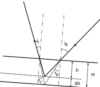
Light produces a bright spot when hitting the surface. From the point of view of the camera, the bright spot is ob-served in the direction corresponding to the angle icwith

re-spect to the normal (Fig. 3): sinip

sinrp

= sinic

sinrc

= nwater (11)

where nwateris the refractive index of water. The difference

in elevation (1h) between the apparent location of the bright spot (h) and the true depth (H ) is obtained by trigonometry, then the true depth can be deduced :

H = 1

1 −tanrp+tanrc

tanip+tanic

1h (12)

The difference between topographies obtained with and without flow will give a distorted bathymetry (1h) that is always shallower than the true bathymetry (H ). Incidence angles can be calculated in any point by simple trigonome-try: ip, ic= f (x,y), and the correction factor in Eq. (12) can

be applied to any point on the surface.

3 Experimental results

Figure 1 is a schematic of the experimental setup used to re-produce microscale braided channels. Details of experiments similar to the ones described here can be found in M´etivier and Meunier (2003). The experiments were conducted at the IPGP experimental facility in a microscale flume made of plexiglass (1.5 m long and 0.75 m wide) with a fully ad-justable bed (height and tilt). The initial slope of the bed was set to approximately 0.05. The sediment in these experiments was composed of glass beads with a D50 of 250 micron and a density of 2500 kg m−3_{. The initial condition for each}

ex-periment was a flat bed with a straight channel (1 cm deep x 2 cm wide) carved down the middle of the bed. The flow was laminar and a fully braided morphology spontaneously developed and reached steady state (sediment input equals sediment output) after several hours. Sediment and water were fed continuously at a constant rate at the upstream end of the flume. Sediment transport was measured at the outlet

(7)

i

_p

i

c

r

_p

r

_c

Δh

H

h

Fig. 3. Light refraction into a water layer.

using a constant head tank which rests on a balance. Flow discharge was typically 2.5 × 10−5_m3_s−1_{and sediment}

dis-charge was typically around 8 × 10−8_m3_s−1_{. Pieces of}

plex-iglass were placed at an angle along the sidewalls in order to deflect the flow and discourage it from sticking to the side-walls. Glare (specular reflection) produced by the free sur-face of water was reduced by using two cross axis polarizers placed in front of the projector and the camera respectively.

3.1 Light3D description, calibration and verification

experiments

The algorithm we used was developed at the Laboratory of Solid State Mechanics of the University of Poitiers, France and is available as a commercial, software package called Light3D. The software allows the user to choose the number of phase-shifted projected patterns (3, 8, 16 or 32) and phase unwrapping can be performed with or without 8 gray code images. The encoded patterns are sent from the computer to a Sanyo PLV-Z5 video-projector. A black and white, 8-bit, 1280 × 1024 pixels µeye Stemmer Imaging CCD cam-era was used for image acquisition. Since light beams are not parallel, the introduced phase shifting is not constant across the whole image. The algorithm implemented into the software recomputes the true phase shifts using Fast Fourier Transform (FFT). Therefore, the need to have a constant grid pitch over the entire image is also overcome. This require-ment is essential when using the Fourier-transform profilom-etry as proposed by Takeda et al. (1982) (Sect. 2.2).

Inside of the rectangular image, the object can be of any shape. The object mask is determined as follows: if the in-tensity of the fringe pattern is the same, this indicates that it is an outside point, so the mask is set to zero and is set to 255 for an inside point if the intensities are different. The phase

is obtained modulo 2π for each internal point (i.e. when mask = 255). Then the phase needs to be unwrapped, but because of the noise or discontinuities, a second mask step is applied, according to a modified Bone algorithm (Br´emand, 1994). This method adopts a “quality” measure to guide the unwrapping path by calculating the second order partial derivatives of the phase map and comparing them to a thresh-old value to detect the discontinuities. A point of discontinu-ity is then set to zero. When the mask procedure is finished, the phase unwrapping algorithm can be applied. Each point having a mask value of 255 should give only one fringe num-ber. If this is not the case, a new threshold is applied until the discontinuity disappears. The image is scanned from one corner, the phase is unwrapped only if at least one of its 8 neighbours is treated. After the first pass, it is possible that several points could not be unwrapped. Then a second pass is performed from the opposite corner, and the cycle is repeated until all the points are analysed.

The phase-shifting technique of generating phase maps combined with a “quality” based unwrapping algorithm makes this method suitable for the measurement of smooth objects with a very high resolution of measurement. When both extended height measuring range and high resolution are required, the software can generate and use 8 gray code images, at the expense of longer acquisition times.

The software allows the unwrapping of absolute phase maps as well as the unwrapping of the difference between two phase maps. The first type of calculation will produce a relief expressed with respect to the reference plane and the second one the relief deformation with respect to an initial state.

For the results shown here the phase field was calculated with 8 phase-shifted images and robust unwrapping using a series of 8 gray code images. Prior to each experiment, a cal-ibration procedure that uses a rotating plane at two positions separated by a given angle was performed to determine the geometric parameters. Two experimental measurements of phase fields were then carried out by means of phase shift-ing. The first one corresponds to the reference plane φref

(position 1 of the calibration board in Fig. 1) and the second one to the same reference plane rotated by an angle β φcal

(position 2 of the calibration board in Fig. 1). The two phase fields obtained for the two positions of the plane are inter-polated by a least square fit considering some (40) different lines distributed into the image, according to the algorithm developed by Breque et al. (2000), and given that the relief of the rotating plane is known in every point. The rotation an-gle β was measured by using a digital slope meter. To begin the unwrapping process, it is necessary to locate the initial fringe, which allows setting the origin O of the working erential. By projecting a single horizontal line onto the ref-erence plane, the alignment of the projector/camera system is adjusted so that the projected line corresponds to the rota-tion axis of the reference plane during calibrarota-tion. The zero fringe is therefore the same in the reference and calibration

(8)

Table 1. Symbols and notations used in this paper

Symbol Description Dimension

I (x,y) intensity of fringe pattern [counts]

a(x,y) background intensity [counts]

b(x,y) local contrast [counts]

c(x,y), c∗(x,y) complex contrast coefficients [counts]

φ (x,y) phase [rad]

φ0(x,y) phase with carrier pattern [rad]

f0 carrier frequency [L]−1

j

√

−1 [0]

F (I ) fourier transform of intensity [L]

A fourier transform of background intensity [L]

C,C∗ fourier transform of contrast coefficients [L]

N number of phase shifts [0]

δi= i2π /N phase shift increment [rad]

Ii(x,y) intensity of fringe pattern for each phase shift [counts]

Z relief [L]

p projected grating spacing [L]

hp projection distance [L]

ho observation distance [L]

d distance between the light source and camera [L]

fp projector focal length [L]

Pr grating pitch at the output lens [L]

γCCD magnification of CCD entrance length [L] /pixel

ip projection incidence angle [rad]

ic camera incidence angle [rad]

rp projection refraction angle [rad]

rc camera refraction angle [rad]

1h difference in elevation between dry and wet relief [L]

H true water depth [L]

nw water refraction index [0]

planes. This simple calibration allows the determination of the geometrical parameters (hp, d, ho, and Pr/fp). These

ge-ometrical parameters are difficult to measure manually and accurately. The precision of the calibration depends on the quality of the calculated phase fields: φref and φcal. A flat,

light color, highly diffusive board was used in the calibration procedure. The results of the calibration were the following:

hp= 2050 mm, d = 1857 mm, ho= 1957 mm, Pr/fp= 0.0051,

for a γCCD= 0.78 mm/pixel.

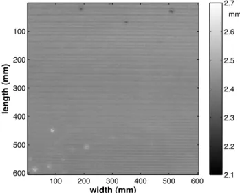
In order to evaluate the precision and resolution of the method, two preliminary experiments were performed. Firstly we analysed the distribution of residual noise of a perfectly flat surface and secondly we discussed the results obtained by demodulation on a object of a known height (a reference scale). In order to obtain a perfectly flat surface we used milk, which has the advantage of being not only flat but opaque and of light colour. Figure 4 shows the results obtained as a difference of 2 levels of milk. One can also see the bubbles that existed on the first surface (black marks) and on the second surface (white marks). Except for the bub-bles zone, the surface was perfectly flat, with a “residual”

width (mm) length (mm) 100 200 300 400 500 600 100 200 300 400 500 600 _2.1 2.2 2.3 2.4 2.5 2.6 2.7 mm

(9)

0 100 200 300 400 500 600 −5 0 5 10 15 20 25 width (mm) height (mm) width (mm) length (mm) 100 200 300 400 500 600 100 200 300 400 500 600 −5 0 5 10 15 20 25 mm a b

Fig. 5. (a) Topography of a stairs object. (b) Cross-section through the object obtained at a length = 230 mm.

modulation still visible. The milk depth level measured on the flat zone has a value of 2.42 mm with a standard devi-ation remarkably low (0.02 mm). This precision is compa-rable to the one reported by using a combination of stereo camera system with structured light illumination (ATOS sys-tem by GOM, France), used in the work of Turowski et al. (2006) (20 µm), and a real improvement with respect to the precision reported by Huang et al. (2010) (0.6 mm).

Figure 5a shows the relief obtained with our reference scale. One can notice the shadow zone behind the object, and the black zones on the top of it where a slopemeter is mounted on. The first stair is 10mm high and the 5 others are 2 mm high. A cross section passing at a length equal to 230 mm is shown in Fig. 5b. As one can notice, the stairs are well resolved. The uncertainty measured on each stair and on the flume board is about 0.1 mm and is mainly due to the non-uniformity of the flume board and of the white painting applied on the scale. The uncertainty on the water depth is the same as on the topography, provided that the water re-fraction is taken into consideration properly (Eq. 12). We verified this statement by introducing our scale into a shal-low tank filled with water and by calculating the water depth from the difference between the topography obtained with and without water.

3.2 Experimental braided channel: topography and

water depth

Bed topography was measured one minute after the flow was turned off (to ensure the bed was uniformly drained). The impact of stopping and starting the flow on bed topography was negligible. Water depth was calculated by differencing the topography obtained with the flow on immediately before it was shut off and with the flow off, taking into account the water refraction as described in Sect. 2.7. This is facilitated in our case by the fact that our experiments are conducted un-der laminar conditions and the slopes are small without steep variations, so that water free surface can be considered uni-form and parallel to bed surface at the scale of moire fringe.

Bed topography and flow depth measured during an exper-iment are shown in Fig. 6. Dry bed topography is between

length (mm) width (mm) water depth 200 400 600 200 400 600 800 1000 −3 −2.5 −2 −1.5 −1 −0.5 0 0.5 1 width (mm) length (mm) dry topography 200 400 600 200 400 600 800 1000 −4 −3 −2 −1 0 1 2 3 4 a) b)

Fig. 6. (a) Bed topography obtained by switching of water flow and (b) water depth.

−4 and 4 mm, while maximum water depth is approximately 3 mm (flow depth increases in the negative direction). Fig-ure 6 shows bed topography and flow depth in cross-section at 530 mm downstream from the top of the study reach. Sev-eral occupied and abandoned channels are visible along this transect.

We excluded data from approximately 25 mm on either side of the flume where the roughness elements were lo-cated. A PDF of flow depth between −2.0 and 2.0 mm was calculated for the study area (red curve in Fig. 8). The av-erage value of the water depth and the standard deviation were −0.24 mm and 0.43, respectively. If we consider pos-itive flow depth noise and if we consider noise distribution as being symmetrical with respect to zero, we obtain the green curve in Fig. 8, which has a standard deviation of 0.28 mm. The difference between total depth distribution and noise results in the true depth distribution shown in blue in Fig. 8. The mean and standard deviation of this distribution are −0.49 and 0.41 mm, respectively. The area of the flume occupied by flow after correcting for noise is 49 %.

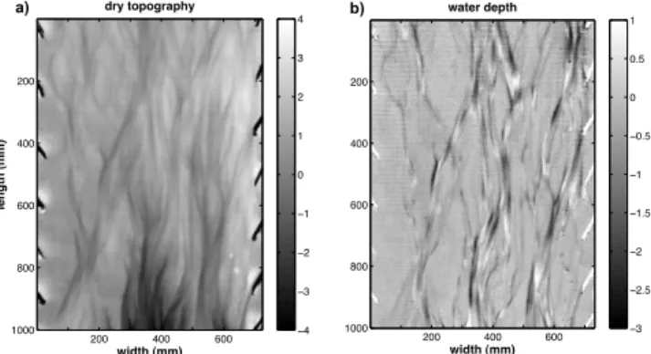
In a separate set of microscale braided river experiments, the focus was on the dynamically evolving topography, and particularly on channel characteristics and dynamics. The study demonstrates how a moir´e method can be used to char-acterize a full range of statistics beyond just topography and depth. Calibration proceeded as above, with slightly different camera distances resulting in 0.93 mm/pixel resolution. Data were again collected via a series of 8 phase-shifted images, and deconstructed with Light3D software. Topography data for the measurements shown here were collected after the system had evolved from a flat bed to the dynamic equilib-rium condition of equal input/output sediment flux, after one hour of steady water and sediment input. The 60 cm by 60 cm focus region of measurements was located in the downstream half of the system, to avoid potential inlet effects. The bulk relief values of this area are characterized in Fig. 9a, gener-ally within a range of −5 mm incision and +2 mm accretion. An initial scan with water running was followed by a scan

(10)

0 100 200 300 400 500 600 700 −4 −3 −2 −1 0 width (mm) topography (mm) wet topography dry topography water depth Abandoned channels Ocuppied channels

Fig. 7. Transects into wet, dry and water depth topographies at length value of 530 mm. −2 −1.5 −1 −0.5 0 0.5 1 1.5 2 0 0.005 0.01 0.015 0.02 0.025 0.03 depth (mm) PDF

total depth distribution noise

water depth distribution

Fig. 8. PDFs of water depth distribution (red curve) with the noise (green curve) removed (blue curve).

taken two minutes after water flow had been stopped, and water depths were determined following the procedure out-lined in Sect. 2.7 (Fig. 9b). Water depth values peak at a value of about 0.5 mm, and vary down to depths of 2–3 mm.

Fig. 9. Histograms of (a) relief values of developed braided river topography and (b) water depth values within channels. Measure-ments are with respect to an initial flat bed.

In this study data were also collected on various aspects of the channels. In order to isolate the channelized areas in a systematic manner, small, noisy water depth values were eliminated by setting a threshold on the water depth data set to only include depths up to the third statistical quartile of depth values (see Fig. 10a for a color-depth image of chan-nelized water depths as isolated by this threshold). Having used this method to isolate the channels, channel charac-teristics such as number, width, length, and spacing were measured. The within-channel slope profiles could also be tracked; see Fig. 9b for profiles of the five longest contin-uous threads of the study region, where it was possible to resolve sub-millimeter-scale features on the channel floors. Additionally, within-channel slopes at the banks were mea-sured perpendicular to flow, as defined over a given distance inward of channel boundaries (Fig. 9c). Measurements such as these can improve our understanding of channel geom-etry organization, especially when combined with informa-tion about local Shields stress and bank migrainforma-tion rate, both of which can be extracted from a time-sequence of relief and water depth data.

Finally, by differencing successive topographic scans (Fig. 11), we can produce a series of maps of erosional and depositional features as they evolve through time. With the high temporal resolution feasible with this method of mea-surement, we can gain new insight into the dynamic evolu-tion of braided rivers.

(11)

Fig. 10. (a) Planview of the analyzed section of the braided river system. Colors correspond to water depth values. The direction of water flow is from the top to the bottom of the image; channel-ized threads are visible as vertical lines. (b) Within-channel ele-vation profiles of the five longest continuous channel threads. Pro-files are plotted from an x-value corresponding to the distance down Sect. (a) at which the channel begins. (c) Histogram of cross-stream slope values within the channels, at the channel banks (outer 3 mm). Channel boundaries are defined using the wet fraction 3rd -quartile threshold discussed in the text.

Fig. 11. (a) Topography scan of a developed braided river system, with flow direction from top to bottom of the image, and (b) scan repeated five minutes later. By subtracting the first scan from the second, we can produce (c) a map of the erosional and depositional features of the landscape.

4 Conclusions

The moir´e method provides a way of characterizing evolving experimental systems at very high spatial and temporal reso-lutions. This detailed description is especially useful for sys-tems as complex and ephemeral as braided rivers, for which patterns of channel organization and feature migration are sensitive to local topographic conditions that vary widely. With high resolution data, dynamic features can be charac-terized with respect to local constraints, and in this way we

can learn about processes that operate at small scales. With significant statistics, we can also identify bulk system pat-terns, and either track their evolution through time or test their sensitivity to changing boundary conditions. Then, with information about both scales of activity, we can hopefully connect the evolution driven by small-scale processes to the emergence of observed large-scale patterns. The ease and resolution of this method of data collection will enable us to describe the evolution and organization of braided river systems with more robust statistics than have yet been re-ported. With this description, we will hopefully be able to parse the relevant processes and timescales that drive braided river evolution.

A certain number of requirements have to be fulfilled in or-der to obtain the best raw images as input data regardless of which method is used for phase measurement. Moir´e meth-ods work well for light color, relatively uniform, diffusive substrate. As in any triangulation method, shadow zones may appear, where all the information is lost. In order to image those zones, the projection and observation angles should be changed. The method is relatively insensitive to stray light since the information is encoded into the phase. Background light should, if possible, be minimized, in order to take full advantage of the dynamic range of elementary detectors of the CCD camera.

Under optimised experimental conditions we report here uncertainties on both topography and bathymetry varying between 20 to 100 µm with sub-millimeter spatial resolu-tion. Under dynamic conditions, due to the fact that this is a multiple-shot method, this uncertainty increases, since the different images are recorded at different moments in time. For time evolving systems, such as the examples shown here, the noise on the water depth distribution increases to about 300 µm, while the uncertainty on the topography stays un-changed, since it is measured without flow, in a frozen con-dition.

Acknowledgements. We thank Y. Gamblin and A. Vieira e Silva

of the Institut de Physique du Globe de Paris for their technical assistance in designing and realizing the experimental set-up. Edited by: D. R. Gr¨ocke

(12)

References

Armstrong, L.: Bank erosion and sediment transport in a microscale straight river, Ph.D. thesis, Universit´e Paris7-Denis Diderot, France, 2003.

Ashmore, P.: Laboratory modelling of gravel bed braided stream morphology, Earth. Surf. Process. Landforms, 7, 201–225, 1982. Aureli, F., Maranzoni, A., Mignosa, P., and C., Z.: Dam-break flows: acquisition of experimental data through an imaging technique and 2-D numerical modeling, J. Hydraul. Eng., 134, 10891101, doi:10.1061/(ASCE)0733-9429(2008)134:8(1089), 2008.

Br´emand, F.: A phase unwrapping technique for object relief determination, Optics and Lasers in Engineering, 21, 49–60, doi:10.1016/0143-8166(94)90059-0, 1994.

Br´emand, F., Doumalin, P., Dupr´e, J., Hesser, F., and Valle, V.: Op-tical Techniques for Relief Study of Mona Lisas Wooden Sup-port, Chap. in: Experimental Analysis of Nano and Engineering Materials and Structures, Springer, Netherlands, 2007.

Breque, C., Brémand, F., and Dupré, J.: Characterization of bio-logical materials by means of optical methods of measurement, in: Second International Conference on Experimental Mechan-ics, edited by Chau, F. and Quan, C., 463–468 pp. , 2000. Breque, C., Dupré, J., and Brémand, F.: Calibration of a

sys-tem of projection moir´e for relief measuring: biomechanical applications, Optics and Lasers in Engineering, 41, 241–260, doi:10.1016/S0143-8166(02)00198-7, 2004.

Cardenas-Garcia, J., Yao, H., and Zheng, S.: 3-D reconstruction of objects using stereo imaging, Opt. Lasers Eng., 22, 193–213, 1995.

Chandler, J. H., Shiono, K., Rameshwaren, P., and Lane, S. N.: Measuring flume surfaces for hydraulics research using a Kodak DCS460, Photogramm. Rec., 17, 39–61, 2001.

Chiang, F.: Moir´e Methods of Strain Analysis, Chap. 6 in: Manual on Experimental Stress Analysis, edited by: Kobayashi, A. S., Soc. for Exp. Stress Anal., Brookfield Center, CT, 51–69 pp., 1983.

Cochard, S. and Ancey, C.: Tracking the free surface of time-dependent flows: image processing for the dam-break problem, Exp. Fluids, 44, 59–71, 2008.

Coleman, S. and Eling, B.: Sand wavelets in laminar open-channel flows, J. Hydraul. Res., 38, 331–338, 2000.

Darboux, F. and Huang, C.: An instantaneous-profile laser scanner to measure soil surface microtopography, Soil Sci. Soc. Am. J., 67, 92–99, 2003.

Devauchelle, O., Malverti, L., Lajeunesse, E., Josserand, C., Lagree, P. Y., and M´etivier, F.: Rhomboid beach pattern: A laboratory investigation, J. Geophys. Res., 115, F02017, doi:10.1029/2009JF001471, 2010a.

Devauchelle, O., Malverti, L., Lajeunesse, E., Josserand, C., La-gree, P. Y., and Thu-Lam, K. N.: Stability of bedforms in lami-nar flows with free-surface: from bars to ripples, J. Fluid Mech., 642, 329–348, 2010b.

Dreano, J., Valance, A., Lague, D., and Cassar, C.: Experimen-tal study of sediment flux controls on transient and steady-state dynamics of bedforms in supply-limited conditions, Earth Surf. Proc. Land., 35, 1730–1743, 2010.

Federici, B. and Paola, C.: Dynamics of channel bifurcations in noncohesive sediments, Water Resour. Res., 39, 1162, doi:10.1029/2005JF000306, 2003.

Ghiglia, D. C. and Pritt, M. D.: Two-dimentional Phase Unwrap-ping: theory, algorithms, and software, Wiley Science, 1998. Guangjun, Z. and Liqun, M.: Modeling and calibration of grid

structured light based 3-D vision inspection, J. Manuf. Sci. Eng., 122, 734–738, 2000.

Halioua, M. and Liu, H.-C.: Optical three-dimensional sensing by phase measuring profilometry, Optics and Lasers in Engineering, 11, 185–215, doi:10.1016/0143-8166(89)90031-6, 1989. Huang, A., Capart, H., Chen, R., and Huang, M.: Laser scanning

technique for the acquisition of digital elevation models of debris flow material, in: Fourth Int Conf on Debris-Flow Hazard Miti-gation, Chengdu, China, September 2007, 539–546 pp., 2007a. Huang, A., Capart, H., Chen, R., and Huang, M.: Experimental

analysis of the seepage failure of a sand slope, in: Fourth Int Conf on Debris-Flow Hazard Mitigation, Chengdu, China, September 2007, 259267, 2007b.

Huang, M., Huang, A., and Capart, H.: Joint mapping of bed eleva-tion and flow depth in microscale morphodynamics experiments, Experiments in Fluids, 1–14 pp., doi:10.1007/s00348-010-0858-4, 2010.

Huntley, J. and Saldner, H.: Shape measurement by temporal phase unwrapping: comparison of unwrapping algorithms, Meas. Sci. Technol., 8, 986–992, 1997.

Kozłowski, J. and Serra, G.: New modified phase locked loop method for fringe pattern demodulation, Opt. Eng., 36, 2025– 2030, 1997.

Kozłowski, J. and Serra, G.: Analysis of the complex phase error introduced by the application of the Fourier transform method, J. of Modern Opt., 46, 957–971, 1999.

Lague, D., Crave, A., and Davy, P.: Laboratory experiments sim-ulating the geomorphic response to tectonic uplift, J. Geophys. Res., 108, 2008, doi:10.1029/2002JB001785, 2003.

Lajeunesse, E., Malverti, L., and Charru, F.: Bed load transport in turbulent flow at the grain scale: Experiments and model-ing, J. Geophys. Res., 115, F04001, doi:10.1029/2009JF001628, 2010a.

Lajeunesse, E., Malverti, L., Lancien, P., Armstrong, L., M´etivier, F., Coleman, S., Smith, C., Davies, T., Cantelli, A., and Parker, G.: Fluvial and Submarine Morphodynamics of Laminar and Near-Laminar Flows: a synthesis, Sedimentology, 57, 1–26, 2010b.

Lancien, P., M´etivier, F., Lajeunesse, E., and Cacas, M.: Incision dynamics and shear stress measurements in submarine channels experiments, in: River, Coastal and Estuarine Morphodynamics 2005, edited by: Parker, G. and Garcia, M. H., Taylor and Francis Group, London, 527–533 pp., 2005.

Liebling, M., Blu, T., and Unser, M.: Complex-wave retrival from a single off-axis hologram, J. Opt. Soc. Am. A, 21, 367–377, 2004. Malverti, L., Lajeunesse, E., and M´etivier, F.: Experimental investi-gation of the response of an alluvial river to a vertical offset of its bed, in: 5th IAHR Symposium on River, Coastal and Estuarine Morphodynamics, edited by: Dohmen-Janssen, C. and Husche, S., 179–184 pp., 2007.

Malverti, L., Lajeunesse, E., and M´etivier, F.: Small is beautifull: upscaling microscale experimental results to the size of natural rivers, J. Geophys. Res., 113, F04004, doi:10.1029/2007JF000,974, 2008.

M´etivier, F. and Meunier, P.: Input and Output mass flux corre-lations in an experimental braided stream. Implications on the

(13)

dynamics of bed load transport, J. Hydrol., 271, 22–38, 2003. M´etivier, F., Lajeunesse, E., and Cacas, M.: Submarine Canyons in

the Bathtube, Journal of Sed. Res., 75, 6–11, 2005.

M´etivier, F., Narteau, C., Lajeunesse, E., Devauchelle, O., Liu, Y., and Ye, B.: A new simple integral technique to analyze bedload transport data, in: 7th IAHR Symposium on River, Coastal and Estuarine Morphodynamics, 179–184 pp., 2011.

Meunier, P.: Braided rivers dynamics, Ph.D. thesis, Institut de Physique du Globe de Paris, 2004.

Ni, W.-J. and Crave, H.: Groundwater drainage and recharge by networks of irregular channels, J. Geophys. Res., 111, F02014, doi:10.1029/2005JF000410, 2006.

Paola, C.: Incoherent Structure: Turbulence as a Metaphor for Stream Braiding, in: Coherent Flow Structures in Open Chan-nels, edited by: Ashworth, P., Bennett, S., Best, J., and McLel-land, S., 705–723 pp., John Wiley & Sons Ltd, 1996.

Paola, C.: Modelling stream braiding over a range of scales, in: Gravel Bed Rivers, edited by: Mosley, M., 11–46 pp., 2001. Paola, C.: Quantitative models of sedimentary basin filling,

Sedi-mentology, 47, 121–178, 2010.

Patorski, K.: Handbook of the moir´e fringe technique, Chap. 10 and 13, Elsevier Science Publishers, 1993.

Pouliquen, O. and Forterre, Y.: Friction law for dense granular flows: application to the motion of a mass down a rough inclined plane, J. Fluid Mech., 453, 131–151, 2002.

Reitz, M. D., Jerolmack, D. J., and Swenson, J. B.: Flooding and flow path selection on alluvial fans and deltas, Geophys. Res. Lett., 37, L06401, doi:10.1029/2009GL041985, 2010.

Rice, C., Wilson, B. N., and Appleman, M.: An instantaneous-profile laser scanner to measure soil surface microtopography, Comput. Electron. Agric., 3, 97–107, 1988.

Sansoni, G., Corini, S., Lazzari, S., Rodella, R., and Docchio, F.: Three-dimensional imaging based on Gray-code light projection: characterization of the measuring algorithm and development of a measuring system for industrial applications, Appl. Opt., 36, 4463–4472, 1997.

Sansoni, G., Carocci, M., and Rodella, R.: Calibration and perfor-mance evaluation of a 3-D imaging sensor based on the projec-tion of structured light, IEEE Trans. Instrum. Meas., 49, 628– 635, 2000.

Sansoni, G., Patrioli, A., and Docchio, F.: OPL-3D: A novel, portable optical digitizer for fast acquisition of free-form surfaces, Review of Scientific Instruments, 74, 2593–2603, doi:10.1063/1.1561602, 2003.

Schmit, J. and Creath, K.: Extended averaging technique for deriva-tion of error compensating algorithms in phase shifting interfer-ometry, Appl. Opt., 34, 3610–3619, 1995.

Schumm, S. A.: The fluvial system, John Wiley & Sons Inc., 1977. Schumm, S. A., Morley, M. P., and Weaver, W. E.: Experimental

fluvial geomorphology, Wiley-Interscience, New York, 1987. Takeda, M.: Spatial-carrier fringe-pattern analysis and its

applica-tions to precision interferometry and profilometry: An overview, Industrial Metrology, 1, 79–99, 1990.

Takeda, M., Ina, H., and Kobayashi, S.: Fourier-transform method of fringe-pattern analysis for computer based topography and in-terferometry, J. Opt. Soc. Am., 72, 156–160, 1982.

Tal, M. and Paola, C.: Dynamic single-thread channels maintained by the interaction of flow and vegetation, Geology, 35, 347–350, 2007.

Turowski, J. M., Lague, D., Crave, A., and Hovius, N.: Experimen-tal channel response to tectonic uplift, J. Geophys. Res., 111, F03008, doi:10.1029/2005JF000306, 2006.

Weiler, M. and Fl¨uhler, H.: Inferring flow types from dye patterns in macroporous soils, Geoderma, 120, 137–153, 2004.