HAL Id: lirmm-00732660
https://hal-lirmm.ccsd.cnrs.fr/lirmm-00732660
Submitted on 16 Sep 2012
HAL is a multi-disciplinary open access
archive for the deposit and dissemination of
sci-entific research documents, whether they are
pub-lished or not. The documents may come from
teaching and research institutions in France or
abroad, or from public or private research centers.
L’archive ouverte pluridisciplinaire HAL, est
destinée au dépôt et à la diffusion de documents
scientifiques de niveau recherche, publiés ou non,
émanant des établissements d’enseignement et de
recherche français ou étrangers, des laboratoires
publics ou privés.
GET_MOVE: An Efficient and Unifying
Spatio-Temporal Pattern Mining Algorithm for Moving
Objects
Nhat Hai Phan, Pascal Poncelet, Maguelonne Teisseire
To cite this version:
Nhat Hai Phan, Pascal Poncelet, Maguelonne Teisseire. GET_MOVE: An Efficient and Unifying
Spatio-Temporal Pattern Mining Algorithm for Moving Objects. 11th International Symposium on
Intelligent Data Analysis (IDA), Oct 2012, Helsinski, Finland. pp.276-288,
�10.1007/978-3-642-34156-4_26�. �lirmm-00732660�
Phan Nhat Hai , Pascal Poncelet , and Maguelonne Teisseire
1
IRSTEA Montpellier, UMR TETIS - 34093 Montpellier, France {nhat-hai.phan,maguelonne.teisseire}@teledetection.fr
2
LIRMM CNRS Montpellier - 34090 Montpellier, France [email protected]
Abstract. Recent improvements in positioning technology has led to a much wider availability of massive moving object data. A crucial task is to find the moving objects that travel together. Usually, they are called spatio-temporal pat-terns. Due to the emergence of many different kinds of spatio-temporal patterns in recent years, different approaches have been proposed to extract them. However, each approach only focuses on mining a specific kind of pattern. In addition to the fact that it is a painstaking task due to the large number of algorithms used to mine and manage patterns, it is also time consuming. Additionally, we have to execute these algorithms again whenever new data are added to the existing database. To address these issues, we first redefine spatio-temporal patterns in the itemset context. Secondly, we propose a unifying approach, named GeT Move, using a frequent closed itemset-based spatio-temporal pattern-mining algorithm to mine and manage different spatio-temporal patterns. GeT Move is implemented in two versions which are GeT Move and Incremental GeT Move. Experiments are per-formed on real and synthetic datasets and the experimental results show that our approaches are very effective and outperform existing algorithms in terms of ef-ficiency.
Keywords: Spatio-temporal pattern, frequent closed itemset, trajectories
1
Introduction
Nowadays, many electronic devices are used for real world applications. Telemetry attached on wildlife, GPS installed in cars, sensor networks, and mobile phones have enabled the tracking of almost any kind of data and has led to an increasingly large amount of data that contain moving objects. Therefore, analysis on such data to find interesting patterns is attracting increasing attention for applications such as movement pattern analysis, animal behavior study, route planning and vehicle control.
Recently, many spatio-temporal patterns have been proposed [1, 3, 4, 6, 14, 10, 12]. In this paper, we are interested in the querying of patterns which capture ’group’ or
’common’behaviour among moving entities. This is particularly true to identify groups of moving objects for which a strong relationship and interaction exist within a defined spatial region during a given time duration. Some examples of these patterns are flocks [1, 2], moving clusters [4, 12], convoy queries [3], closed swarms [6, 9], group patterns [14], periodic patterns [10], etc...
Table 1. An example of a Spatio-Temporal Database Objects ODBTimesets TDB x y
o1 t1 2.3 1.2
o2 t1 2.1 1
o1 t2 10.3 28.1
To extract these kinds of patterns, different algorithms have been proposed. Natu-rally, the computation is costly and time consuming because we need to execute dif-ferent algorithms consecutively. However, if we had an algorithm which could extract different kinds of patterns, the computation costs will be significantly decreased and the process would be much less time consuming. Therefore, we need to develop an efficient unifying algorithm. Additionally, in real world applications (e.g. cars), object locations are continuously reported by using Global Positioning System (GPS). Thus, new data is always available. If we do not have an incremental algorithm, we need to execute again and again algorithms on the whole database including existing data and new data to ex-tract patterns. This is of course, cost-prohibitive and time consuming. An incremental algorithm can indeed improve the process by combining the results extracted from the existing data and the new data to obtain the final results.
With the above issues in mind, we propose GeT Move: a unifying incremental spatio-temporal pattern-mining approach. The main idea of the algorithm and the main contributions of this paper are summarized below.
• We re-define the spatio-temporal patterns mining in the itemset context which en-able us to effectively extract different kinds of spatio-temporal patterns.
• We present approaches, called GeT Move and Incremental GeT Move, which effi-ciently extract FCIs from which spatio-temporal patterns are retrieved.
• We present comprehensive experimental results over both real and synthetic databases. The results demonstrate that our techniques enable us to effectively extract different kinds of patterns. Furthermore, our approaches are more efficient compared to other algorithms in most of cases.
The remaining sections are organized as follows. Section 2 discusses preliminary definitions of the spatio-temporal patterns and the related work. The properties of these patterns are provided in an itemset context in Section 3. We introduce the GeT Move and Incremental GeT Move algorithms in Section 4. Experiments testing effectiveness and efficiency are shown in Section 5. Finally, we draw our conclusions in Section 6.
2
Spatio-Temporal Patterns
2.1 Preliminary Definitions
The problem of spatio-temporal patterns has been extensively addressed over the last years. Basically, spatio-temporal patterns are designed to group similar trajectories or objects which tend to move together during a time interval. Recently, many patterns have been defined such as flocks [1, 2], convoys [3], swarms, closed swarms [6, 9],
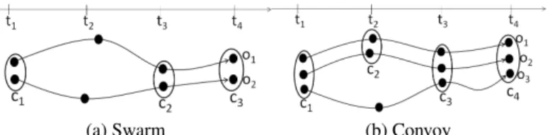
(a) Swarm (b) Convoy
Fig. 1. An example of swarm and convoy where c1, c2, c3, c4are clusters which gather closed
objects together at specific timestamps.
In this paper, we focus on proposing a unifying approach to effectively and ef-ficiently extract all these different kinds of patterns. First of all, we assume that we have a group of moving objects ODB = {o1, o2, . . . , oz}, a set of timestamps TDB =
{t1, t2, . . . , tn} and at each timestamp ti∈ TDB, spatial information3x, y for each
ob-ject. For example, Table 1 illustrates an example of a spatio-temporal database. Usually, in spatio-temporal mining, we are interested in extracting a group of objects staying together during a period. Therefore, from now, O = {oi1, oi2, . . . , oip}(O ⊆ ODB)
stands for a group of objects, T = {ta1, ta2, . . . , tam}(T ⊆ TDB) is the set of
times-tamps within which objects stay together. Let ε be a user-defined threshold standing for a minimum number of objects and minta minimum number of timestamps. Thus|O|
(resp.|T |) must be greater than or equal to ε (resp. mint). In the following, we formally
define all the different kinds of patterns.
Informally, a swarm is a group of moving objects O containing at least ε individu-als which are closed each other for at least minttimestamps. To avoid this redundancy,
Zhenhui Li et al. [6] propose the notion of closed swarm for grouping together both objects and time. A swarm(O, T ) is object-closed if when fixing T , O cannot be en-larged. Similarly, a swarm(O, T ) is time-closed if when fixing O, T cannot be enlarged. Finally, a swarm(O, T ) is a closed swarm if it is both object-closed and time-closed. Then swarm and closed swarm can be formally defined as follows:
Definition 1 Swarm and Closed Swarm [6]. A pair(O, T ) is a swarm if: (1) : ∀tai∈ T, ∃c s.t. O ⊆ c, c is a cluster. (2) : |O| ≥ ε. (3) : |T | ≥ mint. (1)
A pair(O, T ) is a closed swarm if:
(1) : (O, T ) is a swarm.
(2) : �O�s.t.(O�, T) is a swarm and O ⊂ O�.
(3) : �T�s.t.(O, T�) is a swarm and T ⊂ T�.
(2)
For example, as shown in Figure 1a, if we set ε = 2 and mint = 2, we can
find the following swarms({o1, o2}, {t1, t3}), ({o1, o2}, {t1, t4}), ({o1, o2}, {t3, t4}),
({o1, o2}, {t1, t3, t4}). We can note that these swarms are in fact redundant since they
can be grouped together in the following closed swarm({o1, o2}, {t1, t3, t4}).
3
A convoy is also a group of objects such that these objects are closed each other dur-ing at least minttime points. The main difference between convoy and closed swarm
is that convoy lifetimes must be consecutive:
Definition 2 Convoy [3]. A pair(O, T ), is a convoy if: � (1) : (O, T ) is a swarm.
(2) : ∀i, 1 ≤ i < |T |, tai,tai+1are consecutive.
(3)
For instance, on Figure 1b, with ε= 2, mint= 2 we have two convoys ({o1, o2},
{t1, t2, t3, t4}) and ({o1, o2, o3}, {t3, t4}).
Until now, we have considered that we have a group of objects that move close to each other for a long time interval. As shown in [11], moving clusters and differ-ent kinds of flocks virtually share essdiffer-entially the same definition. Basically, the main difference is based on the clustering techniques used. Flocks usually consider a rigid definition of the radius while moving clusters and convoys apply a density-based clus-tering algorithm (e.g. DBScan [5]). Moving clusters can be seen as special cases of convoys with the additional condition that they need to share some objects between two consecutive timestamps [11]. Therefore, in the following, for brevity and clarity sake we will mainly focus on convoy and density-based clustering algorithms.
In [14], Hwang et al. propose a general pattern, called a group pattern, which essen-tially is a combination of both convoys and closed swarms. Basically, group pattern is a set of disjointed convoys which are generated by the same group of objects in different time intervals. By considering a convoy as a timepoint, a group pattern can be seen as a swarm of disjointed convoys. Additionally, group pattern cannot be enlarged in terms of objects and number of convoys. Therefore, group pattern is essentially a closed swarm of disjointed convoys. Formally, group pattern can be defined as follows:
Definition 3 Group Pattern [14]. Given a set of objectsO, a minimum weight threshold minwei, a set of disjointed convoys TS = {s1, s2, . . . , sn}, a minimum number of
convoysminc.(O, TS) is a group pattern if:
� (1) : (O, TS) is a closed swarm with ε,minc. (e.g.|TS| ≥ minc)
(2) : �|TS |i=1 |si|
|TDB| ≥ minwei.
(4)
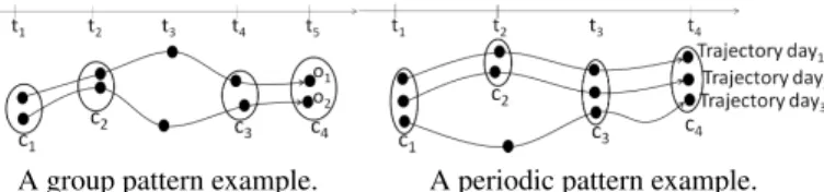
For instance, see Figure 2a, with mint = 2 and ε = 2 we have a set of convoys
TS = {({o1, o2}, {t1, t2}), ({o1, o2}, {t4, t5})}. Additionally, with minc= 1 we have
({o1, o2}, TS) is a closed swarm of convoys because |TS| = 2 ≥ minc, |O| ≥ ε
and(O, TS) cannot be enlarged. Furthermore, with minwei = 0.5, (O, TS) is a group
pattern since |[t1,t2]|+|[t4,t5]| |TDB| =
4
5≥ minwei.
Previously, we overviewed patterns in which group objects move together during some time intervals. However, mining patterns from individual object movement is also interesting. In [10], N. Mamoulis et al. propose the notion of periodic patterns in which an object follows the same routes (approximately) over regular time intervals. For example, people wake up at the same time and generally follow the same route to
A group pattern example. A periodic pattern example. Fig. 2. Group pattern and periodic patten example.
their work everyday. Given that an object’s trajectoryN is decomposed into �N TP�
sub-trajectories.TPis data-dependent and has no definite value. For example,TP can be set
to ’a day’ or ’a year’ depended on different applications. Essentially, a periodic pattern is a closed swarm discovered from�TN
P� sub-trajectories. For instance, in Figure 2b,
we have 3 daily sub-trajectories and from them we extract the two following periodic patterns{c1, c2, c3, c4} and {c1, c3, c4}. As we have provided the definition of a closed
swarm, we will mainly focus on closed swarm mining below.
2.2 Related Work
As we mentioned before, many approaches have been proposed to extract patterns. The interested readers may refer to [11] where short descriptions of the most efficient or interesting patterns and approaches are proposed. For instance, Gudmundsson and van Kreveld [1], Vieira et al. [2] define a flock pattern, in which the same set of objects stay together in a circular region with a predefined radius, Kalnis et al. [4] propose the notion of moving clusters, while Jeung et al. [3] define a convoy pattern.
Jeung et al. [3] adopt the DBScan algorithm [5] to find candidate convoy patterns. The authors propose three algorithms CM C, CuT S, CuT S∗ that incorporate trajec-tory simplification techniques in the first step. The distance measurements are per-formed on trajectory segments of as opposed to point based distance measurements. Then, the authors proposed to interpolate the trajectories by creating virtual time points and by applying density measurements on trajectory segments. Additionally, the convoy is defined as a candidate when it has at least k clusters during k consecutive timestamps. Recently, Zhenhui Li et al. [6] propose the concept of swarm and closed swarm and the ObjectGrowth algorithm to extract closed swarm patterns. The ObjectGrowth method is a depth-first-search of all subsets of ODBthrough a pre-order tree traversal.
To speed up the search process, they propose two pruning rules. Apriori Pruning and
Backward Pruningare used to stop traversal the subtree when we find further traversal that cannot satisfy mintand closure property. After pruning the invalid candidates, a
ForwardClosure checkingis used to determine whether a pattern is a closed swarm. In [14], Hwang et al. propose two algorithms to mine group patterns, known as the Apriori-like Group Pattern mining algorithm and Valid Group-Growth algorithm. The former explores the Apriori property of valid group patterns and extends the Apri-ori algApri-orithm to mine valid group patterns. The latter is based on idea similar to the FP-growth algorithm. Recently in [7], A. Calmeron proposes a frequent itemset-based approach for flock identification purposes.
Even if these approaches are very efficient they suffer the problem that they only extract a specific kind of pattern. When considering a dataset, it is quite difficult, for
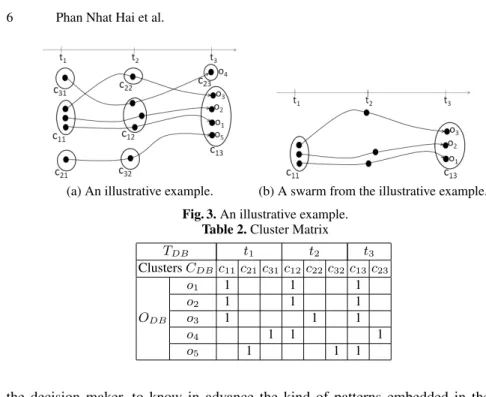
(a) An illustrative example. (b) A swarm from the illustrative example. Fig. 3. An illustrative example.
Table 2. Cluster Matrix TDB t1 t2 t3 Clusters CDBc11c21c31c12c22c32c13c23 ODB o1 1 1 1 o2 1 1 1 o3 1 1 1 o4 1 1 1 o5 1 1 1
the decision maker, to know in advance the kind of patterns embedded in the data. Therefore proposing an approach able to automatically extract all these different kinds of patterns can be very useful and this is the problem we address in this paper and that will be developed in the next sections.
3
Spatio-Temporal Patterns in Itemset Context
Basically, patterns are evolution of clusters over time. Therefore, to manage the evo-lution of clusters, we need to analyse the correlations between them. Furthermore, if clusters share some characteristics (e.g. share some objects), they could be a pattern. Consequently, if a cluster is considered as an item we will have a set of items (called itemset). The main problem essentially is to efficiently combine items (clusters) to find itemsets (a set of clusters) which share some characteristics or satisfy some proper-ties to be considered as a pattern. To describe cluster evolution, spatio-temporal data is presented as a cluster matrix from which patterns can be extracted.
Definition 4 Cluster Matrix. Assume that we have a set of clustersCDB = {C1, C2, . . . , Cn}
whereCi = {ci1ti, ci2ti, . . . , cimti} is a set of clusters at timestamps ti. A cluster
ma-trix is thus a mama-trix of size|ODB| × |CDB|. Each row represents an object and each
column represents a cluster. The value of the cluster matrix cell,(oi, cj) is 1 (resp.
empty) ifoiis in (resp. is not in) clustercj. A cluster (or item)cj is a cluster formed
after applying clustering techniques.
For instance, the data from Figure 3a is presented in a cluster matrix in Table 2. Object o1belongs to the cluster c11at timestamp t1. For clarity reasons in the
follow-ing, cij represents the cluster ci at time tj. Therefore, the matrix cell(o1-c11) is 1,
TDB, ctai ∈ Cai. The support of the itemset Υ , denoted σ(Υ ), is the number of
com-mon objects in every items belonging to Υ , O(Υ ) =�p
i=1ctai. Additionally, the length
of Υ , denoted|Υ |, is the number of items or timestamps (= |TΥ|). For instance, in Table
2, for a support value of 2 we have: Υ = {c11, c12} veryfying σ(Υ ) = 2. Every items
(resp. clusters) of Υ, c11and c12, are in the transactions (resp. objects) o1, o2. The length
of|Υ | is the number of items (= 2). Naturally, the number of clusters can be large; how-ever, the maximum length of itemsets is|TDB|. Because of the density-based clustering
algorithm used, clusters at the same timestamp cannot be in the same itemsets. Now, we will define some useful properties to extract the patterns presented in Sec-tion 2 from frequent itemsets as follows:
Property 1. Swarm.Given a frequent itemset Υ = {cta1, cta2, . . . , ctap}. (O(Υ ), TΥ)
is a swarm if and only if:
� (1) : σ(Υ ) ≥ ε
(2) : |Υ | ≥ mint (5)
Proof. After construction, we have σ(Υ ) ≥ ε and σ(Υ ) = |O(Υ )| then |O(Υ )| ≥ ε. Additionally, as |Υ | ≥ mint and |Υ | = |TΥ| then |TΥ| ≥ mint. Furthermore,
∀taj ∈ TΥ, O(Υ ) ⊆ ctaj, means that at every timestamp we have a cluster containing
all objects in O(Υ ). Consequently, (O(Υ ), TΥ) is a swarm because it satisfies all the
requirements of the Definition 1.
For instance, in Figure 3b, for the frequent itemset Υ = {c11, c13} we have (O(Υ ) =
{o1, o2, o3}, TΥ = {t1, t3}) which is a swarm with support threshold ε = 2 and
mint= 2. We can notice that σ(Υ ) = 3 > ε and |Υ | = 2 ≥ mint.
Property 2. Closed Swarm.Given a frequent itemset Υ = {cta1, cta2, . . . , ctap}. (O(Υ ), TΥ)
is a closed swarm if and only if: (1) : (O(Υ ), TΥ) is a swarm. (2) : �Υ�s.tO(Υ ) ⊂ O(Υ�), T Υ� = TΥ and (O(Υ�), T Υ) is a swarm. (3) : �Υ�s.t.O(Υ�) = O(Υ ), T Υ ⊂ TΥ� and (O(Υ ), TΥ�) is a swarm. (6)
Proof. After construction, we obtain(O(Υ ), TΥ) which is a swarm. Additionally, if
�Υ� s.t O(Υ ) ⊂ O(Υ�), T
Υ� = TΥ and(O(Υ�), TΥ) is a swarm then (O(Υ ), TΥ)
can-not be enlarged in terms of objects. Therefore, it satisfies the object-closed condition. Furthermore, if �Υ� s.t. O(Υ�) = O(Υ ), T
Υ ⊂ TΥ� and(O(Υ ), TΥ�) is a swarm then
(O(Υ ), TΥ) cannot be enlarged in terms of lifetime. Therefore, it satisfies the
time-closed condition. Consequently,(O(Υ ), TΥ) is a swarm and it satisfies object-closed
and time-closed conditions and therefore (O(Υ ), TΥ) is a closed swarm according to
In this paper, we do not provide the properties and proof for convoys, moving clus-ters which are basically extended by adding some conditions to Property 1. For instance, a convoy is a swarm which satisfies the consecutiveness in terms of time condition. For moving clusters [4], they need to share some objects between two timestamps (integrity proportion). Regarding to periodic patterns, the main difference in periodic pattern min-ing is the input data while the property is similar to Property 2. With a slightly mod-ifying cluster matrix such as ”each object o becomes a sub-trajectory”, we can extract periodic patterns by applying Property 2.
Please remember that group pattern is a set of disjointed convoys. Therefore, the group pattern property is as follows:
Property 3. Group Pattern.Given a frequent itemset Υ = {cta1, cta2, . . . , ctap}, a
min-inum weight minwei, a minimum number of convoys minc, a set of consecutive time
segments TS = {s1, s2, . . . , sn}. (O(Υ ), TS) is a group pattern if and only if:
(1) : |TS| ≥ minc. (2) : ∀si, si⊆ TΥ,|si| ≥ mint. (3) :�n i=1si= ∅,� n
i=1O(si) = O(Υ ).
(4) : ∀s �∈ TS, s is a convoy, O(Υ ) �⊆ O(s).
(5) :
�n i=1|si|
|T | ≥ minwei.
(7)
Proof. If|TS| ≥ minc then we know that at least minc consecutive time intervals
si in TS. Furthermore, if∀si, si ⊆ TΥ then we have O(Υ ) ⊆ O(si). Additionally, if
|si| ≥ mintthen(O(Υ ), si) is a convoy (Definition 2). Now, TS actually is a set of
convoys of O(Υ ) and if�n
i=1si = ∅ then TS is a set of disjointed convoys. A little
bit further, if∀s �∈ TS, s is a convoy and O(Υ ) �⊆ O(s) then �TS� s.t. TS ⊂ TS� and
�|TS�|
i=1 O(si) = O(Υ ). Therefore, (O(Υ ), TS) cannot be enlarged in terms of number of
convoys. Similarly, if�n
i=1O(si) = O(Υ ) then (O(Υ ), TS) cannot be enlarged in terms
of objects. Consequently,(O(Υ ), TS) is a closed swarm of disjointed convoys because
|O(Υ )| ≥ ε, |TS| ≥ mincand(O(Υ ), TS) cannot be enlarged (Definition 1). Finally, if
(O(Υ ), TS) satisfies condition (5) then it is a valid group pattern due to Definition 3.
Above, we presented some useful properties to extract spatio-temporal patterns from itemsets. Now we will focus on the fact that from an itemset mining algorithm we are able to extract the set of all spatio-temporal patterns. We thus start the proof process by analyzing the swarm extracting problem. This first lemma shows that from a set of frequent itemsets we are able to extract all the swarms embedded in the database. Lemma 1. LetF I = {Υ1, Υ2, . . . , Υl} be the frequent itemsets being mined from the
cluster matrix withminsup= ε. All swarms (O, T ) can be extracted from F I.
Proof. Let us assume that(O, T ) is a swarm. Note, T = {ta1, ta2, . . . , tam}. According
to the Definition 1 we know that|O| ≥ ε. If (O, T ) is a swarm then ∀tai ∈ T, ∃ctai
s.t. O ⊆ ctai therefore� m
i=1ctai = O. Additionally, we know that ∀ctai, ctai is an
item so∃Υ =�m
i=1ctai is an itemset and O(Υ ) =� m
i=1ctai = O, TΥ =� m i=1tai =
T . Therefore,(O(Υ ), TΥ) is a swarm. So, (O, T ) is extracted from Υ . Furthermore,
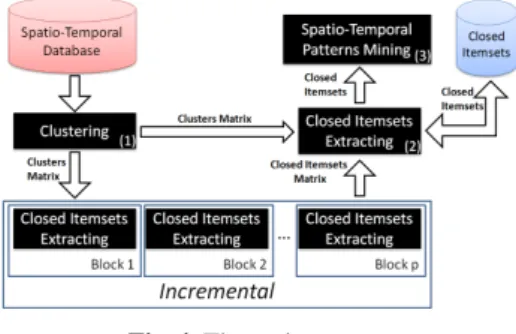
Fig. 4. The main process.
s.t. if(O, T ) is a swarm then ∃Υ s.t. Υ ∈ F I and (O, T ) can be extracted from Υ , we can conclude that∀ a swarm (O, T ), it can be mined from F I.
We can consider that by adding constraints such as ”consecutive lifetime”, ”time-closed”, ”object-”time-closed”, ”integrity proportion” to swarms, we can retrieve convoys, closed swarms and moving clusters. Therefore, the set of all convoys, closed swarms, moving clusters are subset of the set of all swarms. By applying Lemma 1, we retrieve all swarms from frequent itemsets. Consequently, convoys and moving clusters can be completely extracted from frequent itemsets. Additionally, all periodic patterns also can be extracted because they are similar to closed swarms. Furthermore, the following lemma shows that all of group patterns can be extracted from frequent itemsets. Lemma 2. Given F I = {Υ1, Υ2, . . . , Υl} contains all frequent itemsets mined from
cluster matrix withminsup= ε. All group patterns (O, TS) can be extracted from F I.
Proof. ∀(O, TS) is a valid group pattern, we have ∃TS = {s1, s2, . . . , sn} and TS is
a set of disjointed convoys of O. Therefore,(O, Tsi) is a convoy and ∀si ∈ TS,∀t ∈
Tsi,∃cts.t. O⊆ ct. Let us assume Csiis a set of clusters corresponding to si, we know
that∃Υ , Υ is an itemset, Υ =�n
i=1Csiand O(Υ ) =
�n
i=1O(Csi) = O. Additionally,
(O, TS) is a valid group pattern; therefore, |O| ≥ ε so |O(Υ )| ≥ ε. Consequently, Υ
is a frequent itemset and Υ ∈ F I because Υ is an itemset and σ(Υ ) = |O(Υ )| ≥ ε. Consequently,∀(O, TS), ∃Υ ∈ F I s.t. (O, TS) can be extracted from Υ and therefore
all group patterns can be extracted from F I.
4
FCI-based Spatio-Temporal Pattern Mining Algorithm
In this section, we propose two approaches i.e., GeT Move and Incremental GeT Move, to efficiently extract patterns. The global process is illustrated in Figure 4. In the first step, a clustering approach is applied at each timestamp to group objects into different clusters. For each timestamp ta, we thus have a set of clusters Ca = {c1ta, c2ta, . . . , cmta},
with1 ≤ k ≤ m, ckta ⊆ ODB. Spatio-temporal data can thus be converted to a cluster
matrix CM . 4.1 GeT Move
After generating the cluster matrix CM , a FCI mining algorithm is applied on CM to extract all the FCIs. By scanning them and checking properties, we can obtain the
Algorithm 1: GeT Move
Input : int ε, int mint, set of items CDB, double θ, int minc, double minwei 1 begin
2 LCM PatternMining(CDB, ε); 3 PatternMining(X, mint) 4 begin
5 if|X| ≥ mintthen
6 output X; /*Closed Swarm*/
7 gP attern:= ∅; convoy := ∅; mc := ∅; 8 for k:= 1 to |X − 1| do
9 if xk.time= x(k+1).time− 1 then 10 convoy:= convoy ∪ xk; 11 if|T (xk)∩T (xk+1)| |T (xk)∪T (xk+1)| ≥ θ then 12 mc:= mc ∪ xk; 13 else 14 if|mc ∪ xk| ≥ mintthen 15 output mc∪ xk; /*MovingCluster*/ 16 mc:= ∅; 17 else
18 if|convoy ∪ xk| ≥ mintand|T (convoy ∪ xk)| = |T (X)| then 19 output convoy∪ xk; /*Convoy*/
20 gP attern:= gP attern ∪ (convoy ∪ xk); 21 if|mc ∪ xk| ≥ mintthen
22 output mc∪ xk; /*MovingCluster*/ 23 convoy:= ∅; mc := ∅;
24 if|gP attern| ≥ mincand size(gP attern) ≥ minweithen 25 output gP attern; /*Group Pattern*/
26 Where: X is itemset,T (X) is list of tractions that X belongs to, xk.time is time index of item xk, |T (convoy)| is the number of transactions that the convoy belongs to, |gP attern| and size(gP attern) respectively are the number of convoys and the proportion of total length of the convoys in gP attern to TDB.
Algorithm 2: Incremental GeT Move
Input : int ε, int mint, double θ, set of Occurrence sets (blocks) B, int minc, double minwei 1 begin
2 K:= ∅; CI := ∅; 3 foreach b∈ B do
4 CI := CI.update(LCM(b, ε));
5 GeT Move(ε, mint, CI, θ, minc, minwei);
patterns. In this paper, we apply the LCM algorithm [8] to extract FCIs as it is known to be a very efficient algorithm. In LCM algorithm’s process, we discard some useless candidate itemsets. In spatio-temporal patterns, items (resp. clusters) must belong to different timestamps and therefore items (resp. clusters) which form a FCI must be in different timestamps. In contrast, we are not able to extract patterns by combining items in the same timestamp. Consequently, FCIs which include more than 1 item in the same timestamp will be discarded.
Thanks to the above characteristic, we now have the maximum length of the FCIs which is the number of timestamps|TDB|. Additionally, the LCM search space only
depends on the number of objects (transactions) |ODB| and the maximum length of
itemsets|TDB|. Consequently, by using LCM and by applying the above characteristic,
GeT Moveis not affected by the number of clusters and therefore the computing time can be greatly reduced.
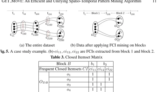
(a) The entire dataset (b) Data after applying FCI mining on blocks Fig. 5. A case study example. (b)-ci11, ci12, ci22are FCIs extracted from block 1 and block 2.
Table 3. Closed Itemset Matrix Block B b1 b2
Frequent Closed Itemsets CI ci11ci12ci22
ODB
o1 1 1
o2 1 1
o3 1 1
o4 1 1
The pseudo code of GeT Move is described in Algorithm 1. The core of GeT Move algorithm is based on the LCM algorithm which has been modified by adding the prun-ing rule and by extractprun-ing patterns from FCIs (line 2). Whenever a closed itemset is detected, the PatternMining sub-function (lines 3-25) is invoked to check properties of the itemset X to extract spatio-temporal patterns.
4.2 Incremental GeT Move
Naturally, in real world applications (cars, animal migration), the objects tend to move together in short interval meanwhile their movements can be different in long interval. Therefore, the number of items (clusters) can be large and the length of FCIs can be long. Additionally, refer to [13, 8], the FCI mining algorithms search space are affected by the number of items and the length of itemsets. For instance, see Figure 5a, objects {o1, o2, o3, o4} move together during first 100 timestamps and after that o1, o2 stay
together while o3, o4move together in another direction. The problem here is that if we
apply GeT Move on the whole dataset, the extraction of the itemsets can be very time consuming.
To deal with the issue, we propose the Incremental GeT Move algorithm. The main idea is to split the trajectories (resp. cluster matrix CM) into short intervals, called blocks. By applying FCI mining on each short interval, the data can then be compressed into local FCIs. Additionally, the length of itemsets and the number of items can be greatly reduced. For instance, see Figure 5, if we consider [t1, t100] as a block and
[t101, t200] as another block, the maximum length of itemsets in both blocks is 100
(instead of 200). Additionally, the original data can be greatly compressed (e.g. Figure 5b) and only 3 items remain: ci11, ci12, ci22.
Definition 5 Block. Given a set of timestampsTDB = {t1, t2, . . . , tn}, a cluster
ma-trixCM . CM is vertically split into equivalent (in terms of intervals) smaller cluster
matrices and each of them is a blockb. Assume Tb is a set of timestamps of block b,
Assume that we obtain a set of blocks B = {b1, b2, . . . , bp} with |Tb1| = |Tb2| =
. . . = |Tbp|,
�p
i=1bi = CM and� p
i=1bi = ∅. Given a set of FCI collections CI =
{CI1, CI2, . . . , CIp} where CIi is mined from block bi. CI is presented as a closed
itemset matrix which is formed by horizontally connecting all local FCIs: CIM = �p
i=1CIi.
Definition 6 Closed Itemset Matrix (CIM). Closed itemset matrix is a cluster matrix
with some differences as follows: 1) Timestampt now becomes a block b. 2) Item c is a
FCIci.
For instance, see Table 3, we have two sets of FCIs CI1= {ci11}, CI2= {ci12, ci22}
which are respectively extracted from blocks b1, b2. We have CIM which is created
from CI1, CI2in Table 3.
Now, by applying FCI mining on closed itemset matrix CIM , we retrieve all FCIs from corresponding data. Note that items (in CIM ) which are in the same block cannot be in the same FCIs.
Lemma 3. Given a cluster matrix CM which is vertically split into a set of blocks B = {b1, b2, . . . , bp} so that ∀Υ, Υ is a FCI and Υ is extracted from CM then Υ can
be extracted from the closed itemset matrixCIM .
Proof. Let us assume that∀bi,∃Ii is a set of items belonging to bi and therefore we
have�|B|
i=1Ii = ∅. If ∀Υ, Υ is a FCI extracted from CM then Υ is formed as Υ =
{γ1, γ2, . . . , γp} where γi is a set of items s.t. γi ⊆ Ii. Additionally, Υ is a FCI and
O(Υ ) =�p
i=1O(γi) then ∀O(γi), O(Υ ) ⊆ O(γi). Furthermore, we have |O(Υ )| ≥ ε;
therefore,|O(γi)| ≥ ε so γi is a frequent itemset. Assume that ∃γi, γi �∈ CIi then
∃Ψ, Ψ ∈ CIis.t. γi ⊆ Ψ and σ(γi) = σ(Ψ ), O(γi) = O(Ψ ). Note that Ψ , γiare from
bi. Remember that O(Υ ) = O(γ1)∩O(γ2)∩. . .∩O(γi)∩. . .∩O(γp) and we have: ∃Υ�
s.t. O(Υ�) = O(γ1) ∩ O(γ2) ∩ . . . ∩ O(Ψ ) ∩ . . . ∩ O(γp). Therefore, O(Υ�) = O(Υ )
and σ(Υ�) = σ(Υ ). Additionally, we know that γ
i ⊆ Ψ so Υ ⊆ Υ�. Consequently,
we obtain Υ ⊆ Υ� and σ(Υ ) = σ(Υ�). Therefore, Υ is not a FCI. That violates the
assumption and therefore we have: if∃γi, γi �∈ CIi therefore Υ is not a FCI. Finally,
we can conclude that∀Υ, Υ = {γ1, γ2, . . . , γp} is a FCI extracted from CM , ∀γi∈ Υ ,
γimust be belong to CIiand γiis an item in closed itemset matrix CIM . Therefore,
Υ can be retrieved by applying FCI mining on CIM .
By applying Lemma 3, we can obtain all the FCIs and from the itemsets, patterns can be extracted. Note that the Incremental GeT Move does not depend on the length restriction mint. The reason is that mint is only used in Spatio-Temporal Patterns
Mining step. Whatever mint(mint≥ block size or mint ≤ block size), Incremental
GeT Move can extract all the FCIs and therefore the final results are the same. The pseudo code of Incremental GeT Move is described in Algorithm 2. The main different between the code of Incremental GeT Move and GeT Move is the update func-tion. In this function, we step by step generate the closed itemsets matrix from extracted closed itemsets in blocks (line 4). Next, we apply GeT Move to extract patterns (line 5).
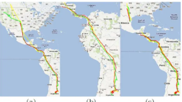
Fig. 6. An example of patterns discovered from Swainsoni dataset. (a) One of discovered closed swarms, (b) One of discovered convoys, (c) One of discovered group patterns.
5
Experimental Results
A comprehensive performance study has been conducted on real datasets and synthetic datasets. All the algorithms are implemented in C++, and all the experiments are carried out on a 2.8GHz Intel Core i7 system with 4GB Memory. The system runs Ubuntu 11.10 and g++ version 4.6.1.
The implementation (source code) is available and also integrated in our online demonstration system4. As in [6], we only report the results on the following datasets5:
Swainsoni datasetincludes 43 objects evolving over time and 764 different timestamps. The interested readers may refer to our online demonstration system2for other experi-mental results. Additionally, similar to [6,3], we first use linear interpolation to fill in the missing data and then DBScan [5] (M inP ts= 2, Eps = 0.001) is applied to generate clusters at each timestamp.
In the comparison, we employ CM C, CuT S∗6[3] (convoy mining) and Object Growth (closed swarm mining). Note that, in [6], ObjectGrowth outperforms V G− Growth [14] (a group patterns mining algorithm) in terms of performance and therefore we will only consider ObjectGrowth and not both.
5.1 Effectiveness
We proved that mining spatio-temporal patterns can be similarly mapped into itemsets mining issue. Therefore, in theoretical way, our approaches can provide the correct re-sults. Experimentally, we do a further comparison, we first obtain the spatio-temporal patterns by applying CM C, CuT S∗, ObjectGrowth as well as our approaches. To apply our algorithms, we split cluster matrix into blocks such as each block b contains 25 timestamps. Additionally, to retrieve all the spatio-temporal patterns, in the reported experiments, the default value of ε is set to 2 (two objects can form a pattern), mint
is 1. Note that the default values are the hardest conditions for examining the algo-rithms. Then in the following we mainly focus on different values of mintin order to
obtain different sets of convoys, closed swarms and group patterns. Note that for group patterns, mincis 1 and minweiis 0.
4www.lirmm.fr/∼phan/index.jsp 5http://www.movebank.org
6The source code of CM C, CuT S∗ is available at
(a) Running time w.r.t. ε (b) Running time w.r.t. mint
(c) Running time w.r.t.|ODB| (d) Running time w.r.t.|TDB|
Fig. 7. Running time on Swainsoni Dataset.
The results show that our proposed approaches obtain the same results compared to the traditional algorithms. An example of patterns is illustrated in Figure 6. For in-stance, see Figure 6a, a closed swarm is discovered within a FCI. Furthermore, from the itemset, a convoy and a group pattern are also extracted (i.e. Figure 6b, 6c). 5.2 Efficiency
In the reported experiments, GeT Move and Incremental GeT Move extract closed swarms, convoys and group patterns while CM C, CuT S∗ only extract convoys and ObjectGrowth only extracts closed swarms. Additionally, all the algorithms are ap-plied on cluster matrices, thus clustering cost was not taken into account.
Efficiency w.r.t.ε, mint. Figure 7a shows running time w.r.t. ε. It is clear that our
approaches outperform other algorithms. ObjectGrowth is the lowest one and the main reason is that with low mint(default mint = 1), the Apriori Pruning rule (the most
efficient pruning rule) is no longer effective. Therefore, the search space is greatly en-larged (2|ODB|in the worst case). Additionally, there is no pruning rule for ε and
there-fore the change of ε does not directly affect the running time of ObjectGrowth. A little bit further, GeT Move is lower than Incremental GeT Move. The main reason is that GeT Move has to process with large number of items and long itemsets. While, thanks to blocks, the number of items is greatly reduced and itemsets are not long as the ones in GeT Move. Figure 7b shows running time w.r.t. mint. In almost all cases, our
ap-proaches outperform other algorithms.
Efficiency w.r.t.|ODB|, |TDB|. Figure 7c-d show the running time when varying
|ODB| and |TDB| respectively. In all figures, Incremental GeT Move outperforms other
algorithms.
In addition, the other experimental results on different real and synthetic datasets are available on our demo system website. Some interesting experiments on the number of patterns, algorithm scalability, optimal block-sizes and also a parameter free version of Incremental GeT Move are integrated on the online system. Interested readers may refer to ”www.lirmm.fr/∼phan/GeTMove.html”.
ferent kinds of spatio-temporal patterns by applying FCI mining techniques. Their ef-fectiveness and efficiency have been evaluated by using real and synthetic datasets. Experiments show that our approaches outperform traditional ones.
One next issue we plan to address is how to take into account the arrival of new objects which were not available for the first extraction. Now, we can store the result to improve the process when new object movements arrive. But, in this approach, we take the hypothesis is that the number of objects remains the same. However in some applications these objects could be different.
References
1. J. Gudmundsson, M.van Kreveld. Computing longest duration flocks in trajectory data. In: GIS 06, New York, NY, USA, pp.35-42.
2. MR. Vieira, P. Bakalov, VJ. Tsotras. On-line Discovery of Flock Patterns in Spatio-Temporal
Data. In: GIS 09, New York, USA, pp.286-295.
3. H. Jeung, ML. Yiu, X. Zhou, CS. Jensen, HT. Shen. Discovery of Convoys in Trajectory
Databases. PVLDB 2008, 1(1):1068-1080.
4. P. Kalnis, N. Mamoulis, S. Bakiras. On Discovering Moving Clusters in Spatio-temporal Data. In SSTD 2005, Angra dos Reis, Brazil, pages 364-381.
5. M. Ester, H.-P. Kriegel, J. Sander, X. Xu. A Density-Based Algorithm for Discovering Clusters
in Large Spatial Databases with Noise. KDD ’96, Portland, pp. 226-231.
6. Z. Li, B. Ding, J. Han, R. Kays. Swarm: Mining Relaxed Temporal Moving Object Clusters. VLDB2010, Singapore, pp. 723-734.
7. A.O.C. Romero. Mining moving flock patterns in large spatio-temporal datasets using a
fre-quent pattern mining approach. Master Thesis, University of Twente, March 2011.
8. T. Uno, M. Kiyomi, and H. Arimura. LCM ver. 2: Efficient mining algorithms for
fre-quent/closed/maximal itemsets. ICDM FIMI 2004.
9. Z. Li, M. Ji, J.-G. Lee, L. Tang, Y. Yu, J. Han, and R. Kays. Movemine: Mining moving object
databases. In SIGMOD 2010, Indianapolis, Indiana, pp.1203-1206.
10. N. Mamoulis, H. Cao, G. Kollios, M. Hadjieleftheriou, Y. Tao, D. W. Cheung. Mining,
In-dexing, and Querying Historical Spatiotemporal Data. SIGKDD’04, pp.236-245.
11. J. Han, Z. Li, L. A. Tang. Mining Moving Object, Trajectory and Traffic Data. In DAS-FAA’10, Japan.
12. C.S. Jensen, D. Lin, and B.C. Ooi. Continuous clustering of moving objects. In KDE(2007), pp. 1161-1174. issn: 1041-4347.
13. C. Lucchese, S. Orlando, R. Perego. DCI Closed: A Fast and Memory Efficient Algorithm to
Mine Frequent Closed Itemsets. ICDM FIMI 2004.
14. Y. Wang, E.-P. Lim, and S.-Y. Hwang. Efficient Mining of Group Patterns from User