Acoustic landmark detection and segmentation using the McAulay-Quatieri Sinusoidal Model

Acoustic Landmark Detection and Segmentation

using the McAulay-Quatieri Sinusoidal Model

by

Tara N. Sainath

B.Sc., Massachusetts Institute of Technology (June 2004)

Submitted to the Department of Electrical Engineering and Computer

Science

in partial fulfillment of the requirements for the degree of

Masters of Engineering in Computer Science and Electrical

Engineering

at the

MASSACHUSETTS INSTITUTE OF TECHNOLOGY

August 2005

@

Massachusetts Institute of Technology 2005. All rights reserved.

A uthor ...

Department of Electrical Engineering and Computer Science

August 16, 2005

Certified by...

Timothy J. Hazen

Research, Scientist, CSAIL

Thes Supervisor

Accepted by.

Arthur C. Smith

Chairman, Department Committee on Graduate Students

BARKER

MASSACHUSETTS INSTMl1JTE OF TECHNOLOGY

AUG

14

2006

Acoustic Landmark Detection and Segmentation using the

McAulay-Quatieri Sinusoidal Model

by

Tara N. Sainath

Submitted to the Department of Electrical Engineering and Computer Science on August 16, 2005, in partial fulfillment of the

requirements for the degree of

Masters of Engineering in Computer Science and Electrical Engineering

Abstract

The current method for phonetic landmark detection in the Spoken Language Systems Group at MIT is performed by SUMMIT, a segment-based speech recognition system. Under noisy conditions the system's segmentation algorithm has difficulty distin-guishing between noise and speech components and often produces a poor alignment of sounds. Noise robustness in SUMMIT can be improved using a full segmentation method, which allows landmarks at regularly spaced intervals. While this approach is computationally more expensive than the original segmentation method, it is more robust under noisy environments. In this thesis, we explore a landmark detection and segmentation algorithm using the McAulay-Quatieri Sinusoidal Model, in hopes of improving the performance of the recognizer in noisy conditions.

We first discuss the sinusoidal model representation, in which rapid changes in spectral components are tracked using the concept of "birth" and "death" of under-lying sinewaves. Next, we describe our method of landmark detection with respect to the behavior of sinewave tracks generated from this model. These landmarks are interconnected together to form a graph of hypothetical segments. Finally, we ex-periment with different segmentation algorithms to reduce the size of the segment graph.

We compare the performance of our approach with the full and original segmen-tation methods under different noise environments. The word error rate of original segmentation model degrades rapidly in the presence of noise, while the sinusoidal and full segmentation models degrade more gracefully. However, the full segmenta-tion method has the largest computasegmenta-tion time compared to original and sinusoidal methods. We find that our algorithm provides the best tradeoff between word ac-curacy and computation time of the three methods. Furthermore, we find that our model is robust when speech is contaminated by white noise, speech babble noise and destroyer operations room noise.

Thesis Supervisor: Timothy J. Hazen Title: Research Scientist, CSAIL

Acknowledgments

I would first like to express my deepest gratitude to my thesis advisor T.J. Hazen. His patience and mentorship over the past year has helped guide me through this thesis. Furthermore, his explanations and insightful suggestions have helped shape me as a researcher.

I would also like to acknowledge Victor Zue and the research staff for welcoming me into the Spoken Language Systems Group and creating a supportive and simulating research environment. Also thank you to Lee Hetherington for his help with the recognizer.

I would like to thank my friends and family for their unwavering love and support; To all the friends I have made over the past 5 years, thank you for making my time at MIT truly rewarding and enjoyable. Thank you to my sister for her patience and her companionship. Thank you to my uncle, aunt and cousins for their constant encouragement and my adorable nieces and nephew for always making me laugh.

Finally, I would like to my parents for being wonderful role models and for always being a source of inspiration in my life.

Contents

1 Introduction

14

1.1 Problem Statement and Motivation . . . . 14

1.2 Noise Robust Speech Recognition . . . . 16

1.2.1 Previous Work . . . . 16

1.2.2 Proposed Noise Robust Technique . . . . 18

1.3 Thesis Goals . . . . 18

1.4 Overview . . . . 19

2 System Components 20 2.1 Speech Recognition Corpora . . . . 20

2.1.1 AV-TIMIT . . . . 20

2.1.2 Noisex-92 . . . . 21

2.2 SUMMIT Speech Recognition System . . . . 22

2.2.1 Mathematical Formulation . . . . 22

2.2.2 Acoustic Model . . . . 23

2.2.3 Pronounciation/Lexical Model . . . . 24

2.2.4 Language Model . . . . 24

2.2.5 Recognition Phase . . . . 25

3 Sinusoidal Modeling of Speech 27 3.1 Acoustic Theory of Speech Production . . . . 27

3.2 The McAulay-Quatieri Algorithm . . . . 28

3.2.2 3.2.3 3.2.4 3.3 Other 3.3.1 3.3.2 3.3.3 Peak-to-Peak Matching . . . . Synthesis . . . . Improvements to Original MQ Algorithm . Sinusoidal Modeling Techniques . . . . Phase Vocoder . . . . Spectral Modeling Synthesis . . . . Harmonic Plus Noise Model . . . . 4 Landmark Detection

4.1 Sinusoidal Model . . . . 4.2 Endpoint Location Method . . . . 4.2.1 Short-Time Energy . . . . 4.2.2 Harmonicity . . . . 4.3 Detecting Landmarks from Sinusoidal Components

4.3.1 Identifying Harmonically Related Sinusoids .

4.3.2 Landmarks from Harmonic Sinusoids . . . .

4.3.3 Landmarks in Unvoiced Regions . . . .

. . . . 29 . . . . 30 . . . . 30 . . . . 32 . . . . 32 . . . . 32 . . . . 33 35 . . . . 35 . . . . 37 . . . . 38 . . . . 40 . . . . 43 . . . . 44 . . . . 45 . . . . 46 5 Segmentation 5.1 Background . . . . 5.2 Full Segmentation . . . . 5.3 Original Segmentation . . . . 5.4 Sinusoidal Model Segmentation . . . . 5.4.1 Segmentation at Voiced/Unvoiced Boundaries . . . . 5.4.2 Segment Connectivity Methods . . . . 5.4.3 Segmentation Using MFCC Distance Information . . . .

6 Experimental Results

6.1 Experimental Setup . . . . 6.2 Sinusoidal Model Landmarks . . . . 6.2.1 Landmark Detection Parameter Settings . . . .

47 47 48 48 50 52 53 54 60 60 61 61

6.2.2 Phonetic Detection Probability . . . . .

6.2.3 Landmark Types Not Used . . . .

6.3 Sinusoidal Model Segmentation Methods . . . .

6.3.1 Voicing Decision Methods . . . .

6.3.2 Connectivity Methods . . . .

6.3.3 MFCC Distance . . . .

6.4 Comparison of Models . . . . 6.4.1 Word-Error-Rate . . . . 6.4.2 Recognition Computation Time... 6.4.3 Word Error Rate vs. Computation Time 6.4.4 Landmark and Segment Comparisons

7 Conclusions

7.1 Sum m ary . . . .

7.1.1 Algorithm Design . . . .

7.1.2 Performance of Sinusoidal Model . . . . 7.2 Future W ork . . . .

A AV-TIMIT Phonemes

B Word Error Rate Tables

B.1 Word Error Rate for White Noise ... B.2 Word Error Rate for Babble Noise ...

B.3 Word Error Rate for Destroyerops Noise . . . . 64 66 67 68 70 70 71 71 76 78 82

86

List of Figures

1-1 Block diagram of a segment-based speech recognition system . . . . . 15

3-1 Block Diagram of Analysis Component [191 . . . .

29

3-2 Birth and Death of Sinusoidal Tracks

[4]

. . . .

30

3-3 Block Diagram of Synthesis Component [191 . . . .

31

4-1 Block Diagram of Landmark Detector . . . . 35

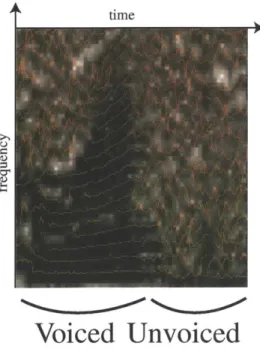
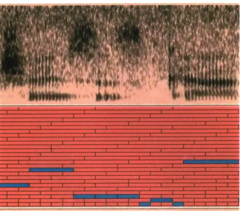
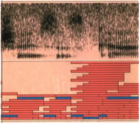
4-2 Typical sinusoidal tracks for voiced and unvoiced speech overlaid on a speech spectogram . . . . 37

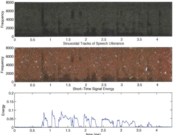
4-3 Sinusoidal Track Representation and Corresponding Signal Energy of Speech Utterance ... ... 39

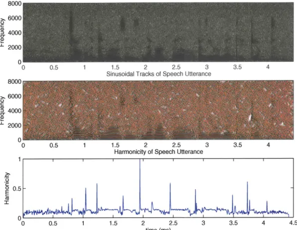
4-4 Sinusoidal Track Representation and Corresponding Harmonicity of Speech Utterance ... ... 41

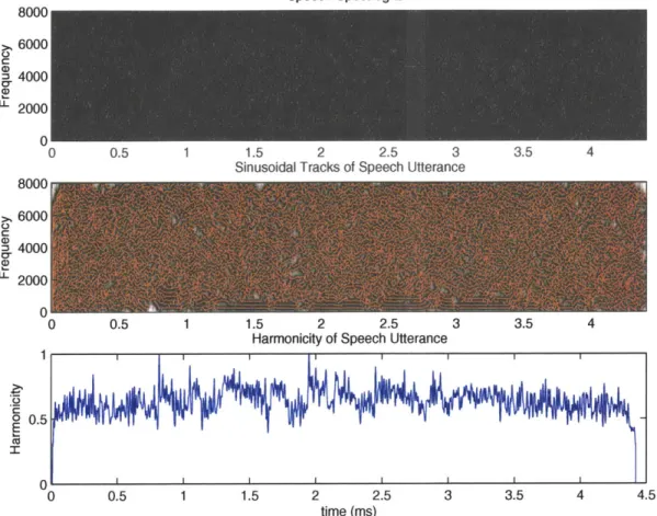
4-5 Sinusoidal Tracks and Harmonicity of Speech with a SNR of -5db. The speech is contaminated by white noise. . . . . 42

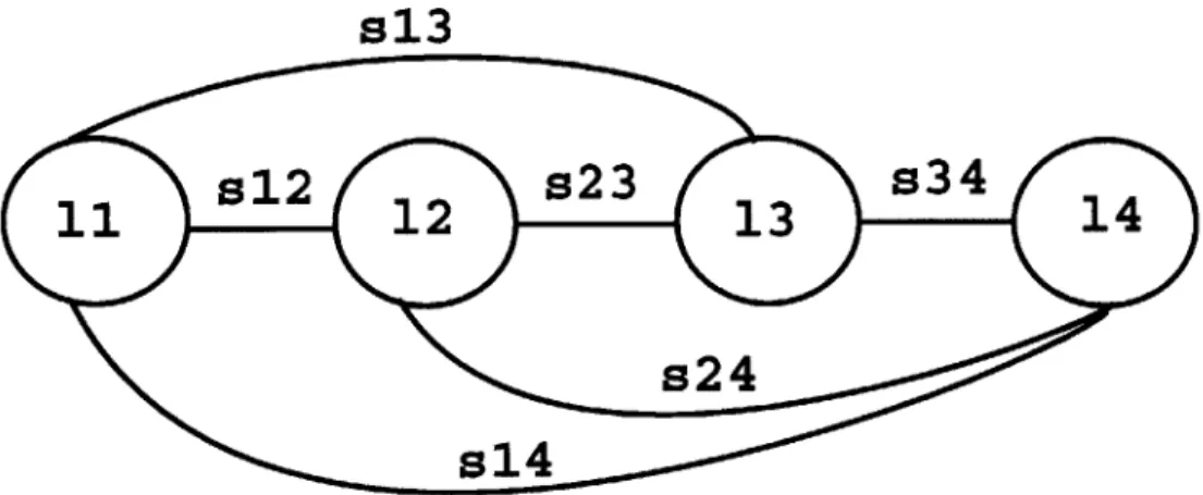
5-1 Segment network for Full Segmentation technique. Each landmark 1i is fully connected to every other landmark

1j

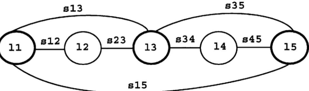
5-3 Segment network for Original Segmentation technique. Major land-marks are indicated in bold. Each minor landmark 1i between major landmarks is fully connected to every other landmark 1j in the graph via segments sij. In addition, each major landmark is connected to two major landmarks forward. . . . . 50 5-4 Graphical display of the segment network for the original segmentation

approach from the SUMMIT recognizer . . . . 51 5-5 Segment network for Sinusoidal Model Two-Connection technique.

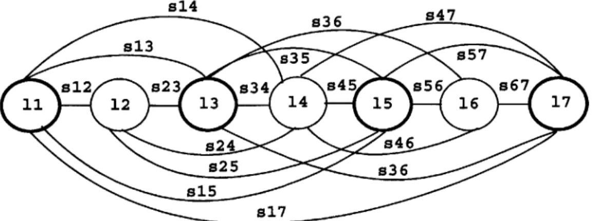
Ma-jor landmarks are indicated in bold. Each minor landmark 1i is con-nected to every other landmark 1j which falls up to two major land-marks away via segments sij. In addition, each major landmark is connected to the next three major landmarks. . . . . 54 5-6 Segment network for Partial-Connection technique. Hard major

land-marks are indicated in bold while soft major landland-marks are embossed. Minor landmarks 1i are connected across a soft major landmarks to other landmarks 1, which falls up to two major landmarks away via segments sij. However, minor landmarks cannot be connected across hard major landmarks. In addition, each major landmark is connected to the next three major landmarks. . . . . 55 5-7 Graphical display of the segment network for the partial-connection

method from the SUMMIT recognizer . . . . 55 5-8 MFCC feature vector distance matrix of a speech signal. . . . . 57 5-9 The top figure shows a major landmark overlaid on top of the speech

signal. Notice the large change in MFCC distance on either side of the major landmark, as illustrated in by the bottom figure. . . . . 58 5-10 The top figure shows a major landmark overlaid on top of the speech

signal. The bottom figure illustrates a small change in MFCC distance on either side of the major landmark. . . . . 59

6-1 Example Receiver Operating Characteristic (ROC) Curve plotting the Probability of Detection, Pd versus the Probability of False Alarm, Pfa 62 6-2 Generated Receiver Operating Characteristic (ROC) Curve for

Land-mark Detection Parameters . . . . 63 6-3 AV-TIMIT phoneme detection probability under clean speech . . . . 65 6-4 Recognition computation time for different segmentation approaches

under varied SNR of white noise . . . . 68 6-5 Word Error Rate for Original Segmentation, Full Segmentation and

Sinusoidal Models for varied SNRs of White Noise . . . . 73 6-6 Word Error Rate for Original Segmentation, Full Segmentation and

Sinusoidal Models for varied SNRs of Babble Noise . . . . 74

6-7 Word Error Rate for Original Segmentation, Full Segmentation and Sinusoidal Models for varied SNRs of Destroyerops Noise . . . . 75 6-8 Recognition computation time for original, full and sinusoidal methods

under varied SNR of white noise . . . . 77 6-9 Word Error Rate vs. Computation Time for Original, Full and

Sinu-soidal Methods. Results are computed for varied vprunenodes parame-ter under 5dB of white noise. . . . . 79 6-10 Word Error Rate vs. Computation Time for Original, Full and

Sinu-soidal Methods. Results are computed for varied vprunenodes parame-ter under 5dB of babble noise. . . . . 80 6-11 Word Error Rate vs. Computation Time for Original, Full and

Sinu-soidal Methods. Results are computed for varied vprunenodes parame-ter under 5dB of destroyerops noise. . . . . 81 6-12 Average time difference between a hypothesized and AV-TIMIT

land-mark for original, full and sinusoidal methods under white noise . . . 83 6-13 Average number of segments across an AV-TIMIT phoneme for

A-1 61 AV-TIMIT phones and corresponding International Phonetic Al-phabet (IPA) Symbols, along with example words using the phonemes 90

List of Tables

6.1 Word Error Rates for Different Sinusoidal Model Segmentation Ap-proaches for varied SNRs of White Noise. Bold represents best seg-mentation method for each noise condition . . . . 69 6.2 Comparison matrix showing results of McNemar's Test for Sinusoidal

Model, Original Segmentation and Full Segmentation methods under varied SNRs of white noise. Methods which are statistically similar are indicated with an ~ symbol and the corresponding significance level. If two methods are statistically different, the model with the better performance is indicated. Also, the model with the lowest error rate for each noise condition is indicated in bold. . . . . 72

B.1 Word Error Rates for Original, Full and Sinusoidal Approaches for varied SNRs of White Noise. Bold represents best method for each noise condition. . . . . 92 B.2 Word Error Rates for Original, Full and Sinusoidal Approaches for

varied SNRs of Babble Noise. Bold represents best method for each noise condition. . . . . 93 B.3 Word Error Rates for Original, Full and Sinusoidal Approaches for

varied SNRs of Destroyerops Noise. Bold represents the best method for each noise condition. . . . . 94

Chapter 1

Introduction

Speech is subject to contamination from many different noise sources. Humans are able to differentiate this speech from noise and comprehend the spoken words. While speech recognition systems are able to successfully process human speech, their per-formance degrades rapidly in the presence of background noise. The purpose of this research is to explore a technique to improve the noise robustness of a segment-based

speech recognition system.

1.1

Problem Statement and Motivation

Most speech recognition systems represent a speech utterance by a temporal sequence of frame-based feature vectors. To date, Hidden Markov Models (HMMs) have been the most dominant frame-based acoustic modeling technique for automatic speech recognition. Although HMMs have proven to be very successful in many tasks, alter-native models have also been developed to address the limitations of HMMs [22].

One type of alternative model that has been developed is a segment-based speech recognizer. The SUMMIT speech recognizer developed by the Spoken Language Sys-tems group at MIT uses a segment-based framework for acoustic modeling [10]. Figure 1-1 shows a block diagram of the SUMMIT recognition system. SUMMIT computes a temporal sequence of frame-based feature vectors from the speech signal, but then hy-pothesizes acoustic landmarks at regions of large change within these feature vectors

speech acoustic segment recognized

signal Landmark landmarks graph Srig words

Detection PISegmentation and flp

Search

Figure 1-1: Block diagram of a segment-based speech recognition system

[9]. These landmarks represent possible transitions between phones.

These landmarks are then connected together to form a graph of possible segmen-tations of the utterance. To minimize the number of interconnections among land-marks, an explicit set of segmentation rules is incorporated into SUMMIT to reduce the size of the segment graph. This graph is passed to scoring and search components which use frame and segment-based measurements to score phonetic hypotheses and find the optimal path of phonetic elements through the segment graph. We will refer to this baseline segmentation algorithm used by SUMMIT as the original segmentation method in this thesis.

While SUMMIT is able to process human speech in noise-free environments, the sys-tem's segmentation algorithm performs poorly in the presence of strong background noises and non-speech sounds. Specifically, the system has a difficult time distinguish-ing between the noise and speech components and often produces a poor alignment of sounds.

Noise robustness in SUMMIT can be improved using a full segmentation method. This technique places landmarks at equally spaced intervals and outputs a segment graph which fully interconnects all landmarks. While this approach is computation-ally more expensive than the original segmentation method, it is more robust under noisy environments.

In this thesis, we investigate a new segmentation algorithm to improve the per-formance of the recognizer under contaminated speech. In addition, we explore alter-native segmentation approaches to reduce computation time but still allow for noise robustness.

1.2

Noise Robust Speech Recognition

In recent years, improvements in speech recognition systems have resulted in high performance of specific tasks under clean conditions. For example, digit recognition has resulted in a less than a 0.5% word error rate. In addition, an error rate of less than 1% has been achieved in an isolated word recognition task [12].

However, the performance of these systems rapidly degrades in noisy environ-ments. For example, the performance of a recognizer in a clean speech environment can drop by over 30% in accuracy when the same speech is corrupted over long-distance telephone lines [20].

Various phenoma occur under noisy conditions which can explain the degradation of these systems [16]. Additive noise alters the speech signal and hence the feature vectors used by speech recognizers to represent this signal. For example, white noise

has been shown to reduce the variance of cepstral coefficients [31].

1.2.1

Previous Work

To date, it has not been possible to develop a universally successful and robust speech recognition system for all environmental conditions. Systems which perform well in one scenario can seriously degrade in performance under a different environmental stress. Therefore, there have been numerous techniques studied to improve the ro-bustness of speech systems under noisy conditions [12]. These techniques can be divided into three main categories based on their objectives:

* Noise Resistant Features

" Speech and Feature Enhancement " Noise Adaptation

Noise Resistant Features

Methods in this category attempt to use features which are less sensitive to noise and distortion. These methods focus on identifying better speech recognition features or

estimating robust features in the presence of noise. While these techniques do not make assumptions nor estimations about noise characteristics, this is sometimes a disadvantage since it is impossible to fully utilize features which are specific to a noise type.

Speech Enhancement

Speech enhancement can be used as a preprocessing step for recognition. These meth-ods attempt to suppress the impact of noise on speech by extracting out clean speech or feature vectors from a contaminated signal. Some approaches include parameter mapping, spectral subtraction, noise masking, comb filtering, Bayesian estimation and parametric spectral modeling. While these techniques are capable of improving recognition performance, oftentimes while the estimated clean speech appears more intelligible to humans it does not necessarily show improvement in the recognizer. Furthermore, it is sometimes difficult to develop a speech enhancement technique capable of suppressing a multitude of noise types.

Noise Adaptation

Instead of deriving an estimate of clean speech, noise adaptation techniques attempt to adapt recognition models to noisy environments. This includes changes to the recognizer formulation, such as changing model parameters of the recognizer, to ac-commodate noisy speech. Parallel Model Combination [7] is one such method for compensating model parameters under noisy conditions in a computationally efficient manner. In addition, some techniques also explore designing noise models within the recognizer itself. While this technique performs well at high SNRs, at low SNRs compensated model signal parameters often show large variances, resulting in a rapid degradation of performance.

1.2.2

Proposed Noise Robust Technique

The previous noise robustness techniques all incorporate an extra stage into the recog-nition process in an attempt to clean up contaminated speech and to improve the scor-ing stage of the recognition process. In this thesis, we attack an orthogonal problem of improving the segmentation phase of the SUMMIT recognition system under noisy conditions. We do not address the problems posed by noise in the feature extraction and acoustic modeling components of the system.

The McAulay-Quatieri Sinusoidal Modeling Algorithm, developed by Tom Quatieri and Robert McAulay [191, models a periodic signal as a collection of sinusoidal com-ponents. Representing a speech signal via this sinusoidal model can help to separate out the harmonic speech components from residual aperiodic noise. Rapid changes in spectral components are tracked using the concept of "birth" and "death" of the underlying periodic sine waves.

We will detect landmarks by looking at the births and deaths of these sinusoids. These landmarks are hypothesized from the sinusoidal behavior of the contaminated speech itself, as opposed to detecting features after applying a speech enhancement technique or using alternative noise resistant features. Landmarks are connected to form a segment graph, an appropriate segmentation algorithm is applied to reduce the size of the search space, and the optimal sequence of phonemes is found based on segment-based measurements derived from the contaminated speech itself.

1.3

Thesis Goals

The overall goal in this thesis is to develop an appropriate landmark detection and segmentation algorithm which provides a good tradeoff between word error rate and computation time under different noise environments. More specifically, one goal of this thesis is to develop a robust landmark detection method that will lead to an improvement in word recognition accuracy over the original segmentation method. Another goal is to develop an appropriate segmentation algorithm to provide faster computation time over the full segmentation approach. In our approach, we detect

landmarks and develop a segmentation algorithm based on the behavior of sinusoidal tracks derived from noisy speech. We hope that our method will be robust to many different noise conditions, a limitation of many previous noise robust techniques.

1.4

Overview

The remainder of this thesis is organized in the following manner. Chapter 2 describes the speech corpora and segment-based system used used for recognition experiments in this thesis. Sinusoidal modeling techniques, including the McAulay-Quatieri Sinu-soidal Modeling Algorithm, will be discussed in Chapter 3. Hypothetical landmarks are detected via a landmark detection method, which is described in Chapter 4. Chap-ter 5 discusses numerous segmentation approaches for the full segmentation, original segmentation and sinusoidal model methods. Chapter 6 compares the word error rate and computation time of the three methods. Finally, Chapter 7 concludes the work in this thesis and provides a few remarks about future work.

Chapter 2

System Components

This chapter describes the speech corpora and segment-based system used used for recognition experiments in this thesis.

2.1

Speech Recognition Corpora

Our recognition experiments use the AV-TIMIT corpus. This corpus contains pho-netically rich and varied audio-visual recordings of read speech. Noisy speech is then simulated by adding noises from the Noisex-92 corpus to the utterances from AV-TIMIT. The following sections describe the corpora in more detail.

2.1.1

AV-TIMIT

The Audio-Visual TIMIT (AV-TIMIT) corpus [14] is a collection of speech recordings developed at the Massachusetts Institute of Technology for research in audio-visual speech recognition. The speech data in AV-TIMIT was recorded with a far-field array microphone and video camcorder in a quiet, controlled office setting. Although the full corpus contains both audio and visual data, the work in this thesis uses only the audio data. One of the main design goals for the corpus was to create a phonetically balanced collection of speech utterances. The TIMIT-SX collection was used to provide a wide range of phonetic contexts of the English language [32]. In

total, 23 different rounds of utterances were created. In each round, a set of 20 sentences is read by a speaker. The first sentence in each round is the same for all speakers to adapt them to recording process, while the other 19 sentences for each round differ. The final corpus contains 223 speakers, including 117 males and 106 females. The total database duration is approximately 4 hours. The sentences from the corpus are divided into three sets:

" The train set consists of 3793 sentences. This is used to train various models used by the recognizer.

" The dev set contains 399 sentences. We used 285 of these utterances to design and develop the sinusoidal model.

" The test set includes 405 sentences. We used 299 of these utterances use to test our developed model.

To create unbiased experimental conditions, the sentences in the train, dev and

test sets do not overlap.

2.1.2

Noisex-92

The Noisex-92 speech-in-noise database [30] was created by the Speech Research Unit at the Defense Research Agency to study the effect of additive noise on speech recognition systems. The database contains the following noises:

" White Noise, Pink Noise, High Frequency Radio Channel Noise " Speech Babble

" Factory Noise

* Military Noises: fighter jets (Buccaneer, F16), destroyer noises (engine room, operations room), tank noise (Leopard, M109), machine gun

In this thesis we look at three specific types of noises, white-noise, speech babble and destroyer operations room noise. The white noise was acquired by sampling a high-quality analog noise generator. The speech babble was obtained by recording samples of 100 people speaking in a canteen. Finally, the destroyer operations room noise was obtained by recording noise samples in an operation room onto a digital audio tape.

We simulate noisy speech by adding noise from the Noisex-92 set to clean AV-TIMIT speech at signal-to-noise ratios in the range of -10db and 20db.

2.2

SUMMIT Speech Recognition System

SUMMIT is a segment-based speech recognition system developed at the Spoken Lan-guage Systems Group at MIT's Computer Science and Artificial Intelligence Labo-ratory [10]. In this section we will briefly discuss the different components of the

SUMMIT recognition system.

2.2.1

Mathematical Formulation

Given a set of acoustic observations A = {ai, a2, a3,..., a,} associated with a speech

waveform, the goal of a speech recognition system is to find the corresponding se-quence of words W = {w1W2...Wn} which has the maximum a posteriori probability

P(WIA). This goal is expressed more formally by Equation 2.1:

= arg max P(WIA) (2.1)

W

In a segment-based recognition system, multiple segmentations, S, are associated with the acoustic observations. For each segmentation, there is an associated sequence of sub-word units U. Sequences of these sub-word units form a corresponding sequence of words, W. Taking into account the segmentation and sub-word units, Equation

2.1 can be rewritten as

W=arg max

Y

S

To simplify computation, SUMMIT uses dynamic programming (e.g., Viterbi) or graph-searches (e.g., A*) to find a single optimal segmentation S, along with an optimal unit sequence

U

W, U,

W,U,s

Applying Bayes rule to the above Equation gives:

P(WjU, SIA)

P(A)

Since P(A) is constant for a given utterance and does not affect the outcome of the search, it is usually ignored. The remaining terms all constitute different components of the SUMMIT recognizer, which will be discussed in the sub-sections below.

2.2.2

Acoustic Model

The term P(A, S|W, U) represents the probability of one specific segmentation and its associated acoustic observations, given the words and sub-word units. In this thesis, we will compute our acoustic observations given a particular segmentation S, to be described in more detail in Chapter 5. Given a particular segmentation S,

P(A, SIW, U) reduces to P(AIS, W, U), which is known as the acoustic model. There are two main types of acoustic modeling approaches used in speech recognition, frame-based and segment-frame-based.

Frame-based Modeling

In frame-based modeling, the acoustic observation space A, consists of a temporal sequence of acoustic frames (e.g. Mel-frequency ceptral coefficients or MFCCs) which

are computed at regular time intervals. To date, Hidden Markov Models (HMMs) have been the most dominant frame-based acoustic modeling technique for automatic speech recognition. However, HMMs have many limitations [22] which alternative models, such as segment-based models, have tried to address.

Segment-based Modeling

In segment-based modeling, frame-level feature vectors (e.g. MFCCs) are computed at regular time intervals, similar to the frame-based modeling approach. However, there is an additional processing stage in segment-based modeling which converts frame-level feature vectors to segmental feature vectors. SUMMIT hypothesizes pho-netic landmarks at regions of large spectral change in the frame-level feature vectors. These variable-length landmarks are connected together to form a collection of possi-ble segmentations of the speech utterance. For a given segmentation S, the acoustic observation space represents the feature vectors associated with S, as well as the feature vectors not associated with S, thus constituting the entire observation space

[10].

2.2.3

Pronounciation/Lexical Model

P(UIW) is the pronunciation or lexical model which gives the likelihood that a

se-quence of sub-word units U, was generated from a given word sese-quence W. This is achieved by a lexical lookup. Each word in the lexicon may have multiple pronunci-ations to account for phonetic variability [13].

2.2.4

Language Model

The language model is denoted by P(W). P(W) represents the a priori probability of a particular word sequence

W

previous n - 1 words, as shown by Equation 2.5:

N

P(W) = P(w1, w2, ... ,w) P(wiWi-1 ... Wn-1) (2.5)

i=1

In this thesis, the language model P(W) is an unweighted word-grammar pair, where a transition from one word to another can only occur if the word pair exists in at least one of the AV-TIMIT sentences [14].

2.2.5

Recognition Phase

Recognition in the SUMMIT system is accomplished by searching a weighted finite-state transducer (FST) [11], which is represented a cascade of smaller FSTs:

R = (S o A) o (C o P o L o G) (2.6)

In Equation 2.6:

" S represents the acoustic segmentation described in Section 2.2.2

" A represents the acoustic observation space

" C relabels context-dependent acoustic model labels as context-independent pho-netic labels

" P applies phonological rules mapping phonetic sequences to phoneme sequences " L represents the lexicon which maps phoneme sequences to words

" G is the language model that assigns probabilities to word sequences

Intuitively, the composition of (C o P o L o G) represents a pronunciation graph

of all possible word sequences and their associated pronunciations. Similarly, the composition of (S o A) is the acoustic segmentation graph representing all possible segmentations and acoustic model labelings of a speech signal. Finally, the compo-sition of all terms in R represents an FST which takes acoustic feature vectors as

input and assigns a probabilistic score to hypothetical word sequences. The single best sentence is found by a Viterbi search through R. If n-best sentence hypotheses are needed, an A* search is then applied.

The search space consists of all possible segmentations of the acoustic features. In order to reduce the size of the search space and computation time of SUMMIT, an explicit segmentation phase is incorporated into the recognizer [18]. The segmentation phase will be discussed in more detail in Section 5.3.

Chapter 3

Sinusoidal Modeling of Speech

In this chapter we describe the acoustic theory behind speech production and the representation of this speech as a collection of sinusoidal components.

3.1

Acoustic Theory of Speech Production

The acoustics of speech production occurs in three distinct stages. First, a source of aooustic energy is created through interactions between airflow from the lungs and the laryngeal and supraglottal structures. Next the source is filtered by the resonant vocal tract cavities. Finally, speech is radiated from the lips [26].

Sources of sound in speech production are produced from three different sources, turbulence noise, vocal fold vibration and transients. Turbulence occurs due to rapid fluctuations in the velocity of airflow at a constriction. This causes the power spec-trum of the noise source to be approximately flat. Turbulence noise can be produced at a constriction at the glottis, creating aspiration noise, or a constriction above the glottis, creating a frication noise. Unvoiced sounds are typically produced from turbulence noise.

Voiced sounds are produced from vocal fold vibration, which is caused by the opening and closing of the glottis. First, the glottis is closed off and pressure is built up behind the constriction. Eventually the pressure will build up and cause the vocal folds to push apart. The rapid airflow across the glottal opening then causes the

pressure to decrease, allowing the vocal folds to close and the cycle to repeat. This periodic opening and closing of the glottis is reflected in periodic glottal pressure and

glottal volume velocity.

Transient sounds occur when there is a high pressure buildup behind a glottal constriction in the vocal tract. When the closure is opened, the pressure is sud-denly released, resulting in a brief transient sound. Plosive bursts are an example of transient sources.

3.2

The McAulay-Quatieri Algorithm

The McAulay-Quatieri (MQ) Algorithm [19] is often used as a sinusoidal representa-tion for sounds. The algorithm assumes that a speech waveform can be represented a collection of sinusoidal components of arbitrary amplitudes, frequencies and phases. For this thesis, we use a MATLAB implementation of the MQ Sinusoidal Model de-veloped by Dan Ellis, an Associate Professor at Columbia [5]. First in the analysis stage, amplitude, phase and frequency parameters are extracted from the speech sig-nal. Next in the peak-matching stage, tracks are formed among peaks which occur at similar frequencies. Finally, in the synthesis stage, extracted parameters are inter-polated together to generate the synthesized speech output. These three sections, as well as extensions to the MQ model, will be discussed in more detail below.

3.2.1

Analysis

In the first step of the MQ Algorithm, amplitude, phase and frequency parameters are extracted from a speech waveform, as shown in Figure 3-1. To extract out these para-meters, first the sampled speech waveform is broken down into a contiguous sequence of windowed frames each of length N, and an N-point short-time Fourier transform (STFT) of each frame is taken. Next, peaks in each STFT frame are found by deter-mining locations where the slope of the waveform changes from positive to negative (concave down) and requiring peaks be at least a relative magnitude threshold below the largest peak in the frame. The MQ algorithm locates the amplitude and frequency

ANALYSIS-SPENCH

INPUJT

FREQUENCIMS PICK~ING APmJE

Figure 3-1: Block Diagram of Analysis Component [19]

for each peak found. The phase is determined by interpolating the unwrapped STFT phases to get exact peak phases for every sample point.

In this thesis, the speech signal was sampled at 16kHz. A 256-point STFT with a 16ms Hamming window was used. Finally, the speech utterance was analyzed at

4ms time intervals. These numbers were chosen to be similar to those used to obtain

the MFCC acoustic feature vectors discussed in Section 2.2.2.

3.2.2

Peak-to-Peak Matching

As the fundamental frequency changes, the number of peaks from frame-to-frame changes. In particular, there is a rapid change in the number and location of peaks during voiced/unvoiced transitions. The concept of sinusoidal "births" and "deaths" is used to account for the movement of spectral peaks between frames. In order to match spectral peaks, tracks are formed by connecting peaks between contiguous frames. A new track is born if the frequency of a peak in the current frame is not within +A of the frequency of a peak in the previous frame. Similarly, a track is dead when there is no peak in the current frame that is within ±A in frequency to a peak in the next frame. A magnitude increase threshold is also imposed so that contiguous peaks at the same frequency which have large magnitude differences are proposed to belong to different tracks. Figure 3-2 shows the birth and death of frequency tracks

birth

eisting

tracks

k

death

new time

peaks

Figure 3-2: Birth and Death of Sinusoidal Tracks [4]

3.2.3

Synthesis

As shown in Figure 3-3, after reducing the speech waveform to a set of sinusoidal

components, the MQ algorithm then synthesizes the waveform by interpolating the

parameters of each track from frame to frame. The amplitude parameter is linearly

interpolated between contiguous frames. However, the phase and frequency

parame-ters cannot be linearly interpolated because these parameparame-ters are obtained modulo

27r. Thus the phase parameter must be unwrapped so that tracks are smooth and

con-tinuous across frame boundaries. In order to smooth out the phase between frames,

the phase is interpolated with a cubic polynomial function, given by Equation 3.1:

0(t)

=+

Yt + at

_t

_(3.1)

To see the mathematics behind solving for the interpolation parameters, see [19].

Finally, after interpolation the sinusoidal tracks are added together to produce a

synthetic speech output.

3.2.4

Improvements to Original MQ Algorithm

The original MQ Algorithm described above has some limitations [6] which newer,

more improved models have tried to address. The sinusoidal model used in this thesis

has been extended to address two of these problems.

SYNTHESIS:

n P"ASES so FRAME-T0-FRAME SEI

OFRECIENCES, LW APNG a GETOR SIN WVES-a-SEC

AMPLQTUDEA

WOTERPOLAT"ON

Figure 3-3: Block Diagram of Synthesis Component

[19]

Lower Energy Threshold

As discussed in Section 3.2.1, peaks in the MQ algorithm are located by determining locations where the spectrum is concave down and at least a relative magnitude threshold below the largest peak in the frame. In regions of quiet speech where the spectrum is relatively flat, using a relative magnitude threshold results in many peaks being detected. Having many peaks detected causes a low amplitude hissing noise in the resynthesized waveform.

To prevent this added background noise, a constant absolute lower threshold is introduced. Thus the final threshold of a frame is the maximum of the largest relative threshold and the absolute lower threshold.

Hysteresis

In the original MQ model, tracks are observed to die out at a specific frequency and to be born again a few frames later at approximately the same frequency. These small tracks which die and appear again most probably belong to the same overall track, but have formed into separate tracks since the magnitude of the track has dropped below the relative magnitude threshold.

To allow tracks of similar frequency to combine into one track, a track amplitude hysteresis parameter is defined to be the lowest magnitude that a track may have without dying out. A larger hysteresis value means a lower magnitude before tracks end, thereby making tracks longer and smoother. Similarly, a smaller hysteresis value

results in smaller tracks.

3.3

Other Sinusoidal Modeling Techniques

Many other methods have been proposed for sinusoidal modeling of sound. In this section, we will discuss three such techniques.

3.3.1

Phase Vocoder

A phase vocoder is used to represent a speech signal as a series of sinusoidal compo-nents [8]. In the analysis stage, the speech signal is broken into windowed frames, and an N-point STFT of each frame is taken. Instead of extracting out the peaks from each SFTF frame as in the MQ algorithm, the phase vocoder considers all N frequency samples within a frame to be important. Therefore, each frame describes the evolution of a sound's frequency components over time. Thus, during the syn-thesis stage, the sound is reconstructed using all N frequency samples within each

frame.

The phase vocoder model is appropriate for sounds with steady harmonic compo-nents. However, sounds with transient and noise components are not well represented using this model. In addition, the vocoder represents a sound at each frame by N time varying sinusoids, but not all these sinusoids are necessary to characterize a sound. For example, harmonic sounds can be modeled only by using sinusoids at integer multiples of a fundamental frequency. The MQ algorithm solves this prob-lem by representing the sinusoids at each frame by the amplitudes and phases of the frequency peaks.

3.3.2

Spectral Modeling Synthesis

The Spectral Modeling Synthesis (SMS) Algorithm, developed at Stanford University, is yet another method for sinusoidal modeling [25]. The SMS method models an input sound s(t) as a sum of sinusoidal components and a noise component, as shown in

Equation 3.2:

k

s(t) =

3

Similar to the MQ algorithm, the sinusoidal components are extracted by inter-polating the spectral peaks. The residual noise is determined by subtracting the synthesized sinusoidal components from the original sound. This stochastic compo-nent is then modeled by filtered white noise, where the filter is determined by fitting a curve to the magnitude spectrum of the noise.

The MQ algorithm was originally used to model speech, but it showed promise for use on a broader class of sounds. However, sound often contains residual components and cannot be reduced to a small number of sine waves. Thus the SMS algorithm provides a more complete model for auditory signals.

3.3.3

Harmonic Plus Noise Model

The Harmonic Plus Noise Model (HNM) [28] models a speech signal s(t) as the sum of a harmonic plus noise component, as shown by Equation 3.3:

s(t) = Sh(t) + sn(t) (3.3)

The harmonic element represents the periodic components of a sound while the noise unit models the non-periodic components. The spectrum is divided into two bands. In the lower band, the signal is modeled by a collection of harmonically related sinusoids. The harmonic component is given by:

K(t)

Sh) Ak(t) cos(kO(t) + 'k) (3.4)

i=1

The signal in the upper band is assumed to be dominated by modulated noise. The noise part is modeled by convolving a time-varying autoregressive (AR) model

h(t, T) with Gaussian white noise b(t) and then modulating the result by an energy envelope function e(t). This noise part is given more explicitly by Equation 3.5:

sn(t)

e(t)[h(t,Tr)

*

b(t)]

(3.5)

The HNM has been used to produce natural-sounding synthetic speech by applying different prosody and spectral envelope modification methods to both components. In addition, the HNM has also been used for smoothing diphone boundaries [27] and most notably in AT&T's Text-to-Speech System [1].

Chapter 4

Landmark Detection

Phonetic landmarks in speech utterances represent change from one phoneme to an-other and are usually identified by regions of large spectral change. In the sinusoidal model, rapid changes in spectral components are tracked using the concept of "birth" and "death" of the underlying sine waves. In order to determine exactly how to detect phonetic landmarks using the sinusoidal model, we look at how phonetic landmarks are placed with respect to the behavior of sinewave tracks generated from this model. The block diagram in Figure 4-1 shows the following steps in our landmark detector. Each of the following blocks will be discussed in the sections below.

4.1

Sinusoidal Model

The first step of the landmark detector is to analyze the speech signal using the sinusoidal model, discussed in Section 3.2. After this stage, we can model our speech signal s[n] as a collection of sinusoidal components given by Equation 4.1:

Figurh

MQ Endpoint oLn a Dto

Sinusoidal Location Landmark Segmentation

signal Model Method Detection Phase network

N

s[n] = ZAk cos(Ok[n] +Vk)

(4.1)

k=1

As discussed in Section 3.1, if the sound source is produced from vocal fold vibra-tions and is voiced, the spectrum will be periodic. A signal which is periodic in time is also periodic in frequency. Furthermore, any periodic signal can be represented by a collection of harmonically related sinusoids, known as the Fourier series [21]. Thus, voiced speech can be represented by a collection of harmonically related sinusoids.

If the sound source is produced by turbulence noise and is unvoiced, the spectrum will be flat and aperiodic. Similarly, the spectrum for transient sources is typically a short duration, intense energy spike. Turbulence and transient sounds can be modeled by a collection of sinusoids which are not harmonically related.

The sinusoidal components given by Equation 4.1 can be broken down into sinu-soids which are harmonically related, representing voiced sound, and those which are not harmonically related, representing unvoiced speech. Equation 4.2 represents this decomposition:

N₁ N₂

s[n]

cos(kOk[n]

+

E

k=1 k=1

voiced unvoiced

Figure 4-2 shows typical sinusoidal tracks for voiced and unvoiced speech regions. Voiced sounds can be adequately estimated by a harmonic collection of sinusoids [23]. In voiced regions, peaks computed from the STFT of the waveform occur at close am-plitudes and frequencies from frame to frame. Since tracks are connected by matching peaks at close frequencies in contiguous frames, the proximity in peak frequencies be-tween frames results in long-duration tracks. In addition, the small amplitude and frequency variation of peaks results in slowly varying, smooth sinusoidal tracks.

According to the Karhunen-Loeve analysis, unvoiced signals can only be suffi-ciently modeled by a very large number of sinusoids [29]. In unvoiced regions, peaks do not occur at close amplitudes or frequencies between neighboring frames. Here, the rapid frequency variation of peaks in unvoiced regions results in many short-duration

time

Voiced Unvoiced

Figure 4-2: Typical sinusoidal tracks for voiced and unvoiced speech overlaid on a speech spectogram

tracks. Furthermore, the rapid amplitude and frequency variation of peaks causes the corresponding sinusoids to exhibit rapid fluctuations as well.

The births and deaths of the long, continuous sinusoids in voiced regions appear to occur at phoneme transitions. However, individual sinusoidal births and deaths can often occur too frequently and randomly to signal a phonetic transition. Therefore, in order to use the sinusoidal model to detect phonemes in voiced regions, voiced and unvoiced regions of the speech utterance must be detected.

4.2

Endpoint Location Method

An important problem in speech processing is to detect voiced speech in the presence of background noise, sometimes referred to as the endpoint location problem

[24].

4.2.1

Short-Time Energy

Short-time energy is often used in speech processing to distinguish between voiced and unvoiced speech segments [24]. The Short-time energy, efn], is defined to be the sum of the squared-magnitude of a windowed speech signal, i.e.:

N

e[n] = E (s[m]w[n - m])2 (4.3)

m=1

where s/nj are the speech samples and w[n] is the window size. In our method, w/n] is chosen to be 12ms.

After the speech utterance is passed through the sinusoidal model, the short-time energy is calculated on the synthesized output. Figure 4-3 shows a sinusoidal track representation for a signal and the corresponding short-time signal energy. When the signal energy is high, the sinusoidal tracks appear to be long and continuous, indicating regions of voicing. However, in unvoiced regions where sinusoidal tracks are short, the signal energy is usually very low. Voiced and unvoiced speech can often be differentiated by a corresponding low or high signal energy.

While the short-time energy or spectral energy has been conventionally used to distinguished between voiced and unvoiced segments, this measure becomes less re-liable and robust in noisy environments [17]. Specifically, in noisy environments the signal energy is weak for particular phonemes, making it difficult to accurately detect regions of voicing. The phonemes for which it was was problematic to locate an exact endpoint include the following:

1. weak fricatives (/f, th, h/) at the beginning and end of a segment 2. weak plosive bursts for /p, t, k/

3. segment final nasals /n, m, q/ 4. weak semivowels /r, y, 1, w/

Therefore to obtain a more accurate estimation of voicing decisions, it is necessary to use an additional technique to identify voicing regions, which will be discussed in

Speech Spectrogram

0.5 1 1.5 2 2.5 3 3.5 4 Sinusoidal Tracks of Speech Utterance

0 0.5 1 1.5 2 2.5 3 3.5 4 Short-Time Signal Energy

0 0.5 1 1.5 2

time (ms)

2.5 3 3.5 4

Figure 4-3: Sinusoidal Track Representation and Corresponding Signal Energy of Speech Utterance 8000 6000 4000 2000 0 0 8000 6000 4000 2000 0 C C U-0 0. 0.1 0. 0.0 2 - I I I I I I 1 5-1 - \ 5 -MWQMM I - - -- IMBHIM

the next section.

4.2.2

Harmonicity

Harmonicity is a measure of the strength of the pitch perception for a sound. Voiced regions can be modeled by a collection of harmonically related sinusoids, and thus contain high harmonicity. However, unvoiced regions are modeled with non-harmonic sinusoids and contain very little harmonicity. To exploit this difference, a harmonicity calculation is often used to detect regions of voiced and unvoiced speech segments. Harmonicity can be calculated as the the ratio of harmonic energy to signal energy, as given by Equation 4.4:

Sh [n]

n?] , 0 < h[n] < 1 (4.4)

To compute the energy of the harmonic signal, Sh, first the fundamental frequency of the synthesized waveform is calculated. We will discuss the method for fundamental frequency calculation in more detail in Section 4.3.1. The harmonic signal is calculated by finding the sinusoids which are integer multiples of the fundamental frequency.

Figure 4-4 shows a speech signal and its corresponding harmonicity. The har-monicity often peaks when transitioning into a voiced region since the harmonic energy is very large at the start of a voiced phrase. Similarly, the harmonicity tends to reach a minimum when entering an unvoiced region as the harmonic energy is very low.

Using harmonicity alone to identify regions of voicing has some disadvantanges. For example, as the SNR increases, the peaks and valleys of the harmonicity become more subdued. Figure 4-5 shows the harmonicity for the same speech signal shown in Figure 4-4, now corrupted by noise. The increased noise causes many small local peaks and valleys, which are often falsely detected to be voiced or unvoiced regions respectively.

However, whenever the harmonic energy is strong or weak, the harmonicity tends to peak or dip respectively. Especially in regions of weak voicing where the

short-Speech Spectrogram

0 0.5 1 1.5 2 2.5 3 3.5 4

Sinusoidal Tracks of Speech Utterance

8000 6000 = 00 C 4000 2000 0 8000 6000 4000 Cr U 2000 0 0 0. 1 0.5

Figure 4-4: Sinusoidal Track Representation and Corresponding Harmonicity of

Speech Utterance

0 0.5 1 1.5 2 2.5 3 3.5 4

Harmonicity of Speech Utterance

) 0.5 1 1.5 2 2.5 3 3.5 4 4.5

Speech Spectrogram 8000 6000 C (D=4000 L2000 0 0 0.5 1 1.5 2 2.5 3 3.5 4

Sinusoidal Tracks of Speech Utterance

8000 6000 C) =4000 U-2000 0 0 0.5 1 1.5 2 2.5 3 3.5 4

Harmonicity of Speech Utterance

0 C M 1 0.5

U0

Figure 4-5: Sinusoidal Tracks and Harmonicity of Speech with a SNR of -5db. The

speech is contaminated by white noise.

time energy does not provide a precise voicing decision, the harmonicity is more prominent and often helps to yield a more accurate voicing detection. Therefore, the signal energy may be used to identify general areas of voicing, but the harmonicity can help to make the areas of voicing more precise.

4.3

Detecting Landmarks from Sinusoidal

Compo-nents

In order to determine exactly how to detect phonetic landmarks using the sinusoidal model, we look at how phonetic landmarks from AV-TIMIT waveforms are placed with respect to the behavior of sinewave tracks generated from the sinusoidal model. A few important observations are drawn by looking at the location of these landmarks with respect to the locations and behaviors of the sinusoidal tracks. These observations include:

" In Voiced Regions:

1. Sinusoids tend to be long, smooth and slowly-varying

2. A region with a lot of harmonically born sinusoids usually represents the beginning of a voiced region

3. A region with a lot of harmonically dead sinusoids usually represents the transition from voiced to unvoiced region.

4. Oftentimes sinusoidal births and deaths are not present when transition-ing into a semivowel or nasal, or when transitiontransition-ing from one vowel into another

" In Unvoiced Regions:

1. Sinusoids tend to be short and rapidly-varying

2. Births and deaths of sinusoids occur frequently and randomly with respect to AV-TIMIT phonetic landmarks

With these observations in mind, the method for detecting phonetic landmarks from sinusoidal components in voiced and unvoiced regions will be described in the following sections.

4.3.1

Identifying Harmonically Related Sinusoids

In voiced regions, phonetic landmarks are detected from the births and deaths of sinusoids. Sometimes there are not breaks in sinusoidal tracks when transitioning between particular voiced phonemes, but there is usually a break in harmonically related sinusoids. The births and deaths of harmonically related sinusoids, which are obtained from knowledge of the fundamental frequency, allow us to more accurately detect landmarks rather than just the sinusoidal tracks alone. In this section, we will describe the method for obtaining harmonic sinusoids.

Fundamental Frequency

In order to detect harmonic sinusoidal components, it is first necessary to identify regions where sinusoids are harmonically related to the fundamental frequency. One way of estimating the fundamental frequency of a speech segment is to compute the cepstrum. The cepstrum is a Fourier analysis of the logarithmic amplitude spectrum of the signal. If the log amplitude spectrum contains many regularly spaced harmon-ics, then the cepstrum will show a peak corresponding to the fundamental frequency of these harmonics.

To obtain the fundamental frequency of a speech signal, the waveform is broken into frames and the fundamental frequency for each frame is computed by finding the peak in the cepstrum of the frame. Accurately detecting the pitch period of a speech signal is difficult for several reasons [3]. For example, signals are not always completely periodic and can be corrupted by noise. Therefore, we take the most dominant peak of the cepstrum in each frame to calculate the fundamental frequency.

Harmonically Related Sinusoids

After the fundamental frequency for the waveform is computed, sinusoidal tracks which occur at frequencies that are multiples of the pitch are identified to be harmon-ically related sinusoids. As shown in Figure 4-3, the higher energy speech harmonics at low frequencies are less corrupted by noise and their long, smooth behavior tends to indicate phonetic transitions. However, high frequency harmonics are typically lower in energy and are more corrupted by noise, therefore providing little informa-tion about phonetic transiinforma-tions. Therefore for the purposes of detecting landmarks from sinusoidal components, harmonic sinusoids are only detected at low frequency regions, up to 4 kHz.

4.3.2

Landmarks from Harmonic Sinusoids

After harmonically related sinusoids are identified in regions of voicing, the next step is to detect phonetic landmarks from the births and deaths of these tracks. First, the number of sinusoids that are born or die at a set frame interval of 12ms is counted. However not all sinusoidal births and deaths correspond to potential phonetic land-marks. For example, when transitioning into the beginning of a voiced region, various sinusoids may not be born at the exact same instance, but rather there is a sequence of staggered births. Furthermore, noise may influence sinusoidal tracks and cause them to break at certain frames but this usually does not correspond to a phonetic landmark. Therefore, the optimal number of harmonic births which constitute a po-tential phonetic landmark must be determined. In addition, the optimal number of harmonic deaths to identify a potential phonetic landmark must also be calculated. We will discuss our method for determining these optimal numbers in Section 6.2.1.

In addition, we further make the assumption that if a harmonically born landmark is detected, another harmonically born landmark will not be detected for at least a certain number of frames future frames. This parameter will be referred to as born hop. Similarly, if a harmonically dead landmark is detected, another similar landmark will not be detected for at least a specified of frames, known as dead hop. Again, we