$Q\FRUUHVSRQGHQFHFRQFHUQLQJWKLVVHUYLFHVKRXOGEHVHQWWRWKHUHSRVLWRU\DGPLQLVWUDWRU WHFKRDWDR#OLVWHVGLIILQSWRXORXVHIU
2SHQ$UFKLYH7RXORXVH$UFKLYH2XYHUWH2$7$2
2$7$2 LV DQ RSHQ DFFHVV UHSRVLWRU\ WKDW FROOHFWV WKH ZRUN RI VRPH 7RXORXVH UHVHDUFKHUVDQGPDNHVLWIUHHO\DYDLODEOHRYHUWKHZHEZKHUHSRVVLEOH
7KLVLVYHUVLRQSXEOLVKHGLQ
7RFLWHWKLVYHUVLRQ
2IILFLDO85/
an author's https://oatao.univ-toulouse.fr/11391
https://doi.org/10.1109/RADECS.2008.5782739
Goiffon, Vincent and Hopkinson, Gordon R. and Magnan, Pierre and Bernard, Frédéric and Rolland, Guy and Saint- Pé, Olivier Multi level RTS in proton irradiated CMOS image sensors manufactured in deep submicron technology.
(2008) In: Radiation Effects on Components and Systems - RADECS, 10 September 2008 - 12 September 2008 (Jyväskylä, Finland).
Multi level RTS in proton irradiated CMOS image sensors manufactured in deep submicron technology
V. Goiffon G. R. Hopkinson, P. Magnan, F. Bernard, G. Roland, and O. Saint-P´e
Abstract—A new automated method able to detect multi level random telegraph signals in pixel arrays and to extract their main characteristics is presented. The proposed method is applied to several proton irradiated pixel arrays manufactured using a 0.18μm CMOS process dedicated to imaging. Despite the large proton energy range and the large fluence range used, similar exponential RTS amplitude distributions are observed. A universal mean amplitude is extracted from these distributions and the number of RTS defects appears to scale well with total NIEL. These conclusions allow the prediction of RTS amplitude distributions. The effect of electric field on RTS amplitude is also studied and no significant relation between electric field and RTS amplitude is observed.
Index Terms—Random telegraph signal, RTS, proton irradi- ation, CMOS image sensors (CIS), active pixel sensors (APS).
I. INTRODUCTION
D
ISPLACEMENT damage induced random telegraph sig- nal (RTS) in the image sensor dark current has been studied during the last fifteen years [1]–[9]. All these studies revealed that this kind of RTS is caused by metastable bulk defects located in the depleted volume of the semiconductor.These defects seem to be universal since it has been observed with the same behavior in image sensors manufactured using several CCD and CMOS technologies [9]. Its discrete switch- ing amplitudes are known to be proportional to integration time, and several theories are proposed to explain their unex- pected high values. Among these, electric field enhancement is the most cited justification of such an intense generation process.
Most of the detection methods used to study RTS pixels are based on amplitude and/or standard deviation thresholds. The use of such techniques limits the number of detectable RTS pixels, and the number of parameter that can be automatically extracted. Therefore, not many studies exist on a large number of multi level RTS. We developed a method based on an edge detection technique to automatically detect multi level RTS and extract their typical characteristics.
After reviewing the existing RTS detection techniques and presenting our motivations to develop a new one, the proposed method is described. In a third part, the first results of this method are presented on unirradiated and irradiated arrays.
V. Goiffon and P. Magnan are with Universit´e de Toulouse, ISAE, Toulouse, 31055, France (Phone: +33 5 6133 8251, Fax: +33 4 6133 8345, e-mail:
G. Hopkinson is with Surrey Satellite Technology Limited, Sevenoaks, TN14 5LJ, United Kingdom.
F. Bernard and G. Roland are with CNES, Toulouse, 31401, France.
O. Saint-P´e is with EADS Astrium, Toulouse, 31402, France.
Despite the variety of exposure conditions, an exponential amplitude distribution is observed with a constant mean am- plitude. The number of RTS defects appears to scale with total NIEL and a significant number of more than 2-level RTS are observed, even on an unirradiated device. Finally, the same measurement are repeated with several photodiode bias conditions. The applied electric field does not seem to have any effect on RTS amplitude whereas it decreases the mean dark current pedestal on which the RTS is superimposed.
II. MULTI LEVELRTSDETECTION
A. Existing RTS detection methods
Multi level RTS can be described by the following pa- rameters: the number of discrete levels, the amplitude each transition, the characteristic time constants and the mean dark current pedestal on which the discrete fluctuations are superimposed. Two types of time constants can be define. First the level time constants are the mean time spent on each level.
Second, the transition time constant from level n to levelm can be defined as the mean time before a transition from level nto levelmoccurs.
The following RTS detection methods have been reported:
visual counting [2], threshold based methods [4], [7], value histogram analysis [6], statistical properties analysis [10] and the non scattering pattern method (NSP) [11]. Tab. I compares these techniques to the method we propose in this paper.
Visual counting and NSP methods main drawbacks are that they can not be automated and that they depend on the operator appreciations. Threshold based method most often use a criterion on standard deviation, mean dark current or both to decide what signals are RTS. This is most probably the fastest automated way to count RTS pixels but such methods do not provide RTS characteristics. These techniques can be objective, but it has been referred to as non objective method in the table since most of the time the threshold is manually tuned for each device and/or each test condition to minimize the false alarm probability. Histogram based methods appear to be a good compromise but the decision threshold margin is usually large (five times the standard deviation is cited in [6]) which can be a problem to discriminate the RTS levels. Like the threshold based methods, they are also very sensitive to low frequency drift which are often observed on long duration RTS measurements. Such drifts change the shape of the value histograms and reduce significantly the detection efficiency.
For standard deviation threshold based methods, these drifts can lead to high standard deviation and will be counted as RTS. Yuzhelevskiet al.statistical method has been developed
COMPARISON OFRTSDETECTION AND PARAMETER EXTRACTION METHODS. FOR EACH METHOD,THE FOLLOWING FEATURE ARE USED AS
CRITERIA FOR THE COMPARISON: RTSDETECTION,AUTOMATED DETECTION,OBJECTIVE DETECTION,NUMBER OF LEVEL EXTRACTION, LEVEL VALUE EXTRACTION,LEVEL TIME CONSTANT EXTRACTION AND
TRANSITION TIME CONSTANT EXTRACTION.
Method Detect. Auto. Object. Level Time const.
No. Val. Lvl. Trans.
Visual yes no no yes yes yes yes
Threshold yes yes no no no no no
Histogram yes yes yes yes yes no no
Statistics no - - ? yes yes ?
NSP yes no no yes yes yes no
Egde det. yes yes yes yes yes yes yes
to reconstitute 2-level RTS. It supposes that the studied signal has already been identified as RTS and it is not clear if the method can be extended to multi level RTS.
The proposed method is based on the detection of sharp edges in the signal. The detection criterion is universal and does not need to be tuned. If such edge is detected, the signal is considered as RTS. The dark current values before and after each encountered edge gives the level before and after the transition. The time separating two edges gives the inter transition time. Therefore, all the needed parameters can be extracted. Low frequency drifts can affect the level discrimination but does not affect the RTS detection process.
One can note that only one RTS transition is needed to trigger the detection in contrast to most of the cited methods.
B. Proposed detection method
1) Method principle: As presented in Fig. 1, an ideal random telegraph signal can be represented as the succession of rising and/or falling edges in a white Gaussian noise (WGN) background. Like in signal processing applications, the detec- tion of these edges can be done thanks to the convolution of a normalized step shaped filter and the studied signal. The numbers of coefficients are the same before and after the rising edge. On the high or low state, the coefficient values are equal to each other and their sum absolute values are equal to1. The filter length reduces the white noise by averaging it whereas the difference between the high and low state values amplifies any encountered edge. The filter output (see Fig. 1) illustrates these properties. The convolution process generates triangles when an edge is encountered. Measuring the peak height of these triangles allows to retrieve the step amplitude.
In order to guaranty a good detection efficiency with a reduced probability of false alarm, the detection condition was set to Astep> σsig, withAstepthe step amplitude andσsigthe signal standard deviation. Three cases have to be addressed to verify the relevance of this condition. First if the WGN standard deviation σwn is much lower than the step amplitude Astep
then
Astep>> σwn⇒σsig≈Astep/2. (1) Second, if the RTS amplitude is close to the white noise level Astep≈σwn⇒σsig≈σwn≈Astep/2. (2)
0 500 1000 1500
−1 0 1 2
Samples
Signal (AU) Filtered signal
2 level RTS signal
Fig. 1. Method principle illustration. A classical 2-levels RTS signal and the same signal after being filtered by the normalized step filter are shown.
The dashed lines represent the detection threshold and are equal to the signal standard deviation. AU stands for arbitrary unit.
Since Astep > Astep/2, RTS will be effectively detected in the two previous cases. Finally, if the RTS amplitude is much smaller than the noise background or if there is no RTS at all Astep<< σwn⇒σsig≈σwn. (3) ThereforeAstep<< σsigand this signal will not be recognized as RTS. To summarize, this objective criterion allows to detect 100% of discrete fluctuations greater or equal to the white noise background and does detect0% of signal with no RTS behavior. Between these two cases, some small RTS signals will be detected and some others will not, like during a visual inspection. This “dead” zone can not be avoided and is not very important since white noise dominates these signals.
An objective fully automated detection is achieved by filter- ing sequentially every signal to analyze, storing the maximum filter output value for each signal and compare it to the detection thresholdσsig. Such an algorithm works well if the filtering process is perfect. It means thatAstepmust precisely represent the step amplitude. This suggests two key limitations.
First the filter has to be long enough to attenuate the white Gaussian noise sufficiently. Indeed, if it is not enough reduced, the white noise can trigger the detection process by crossing the dashed line in Fig. 1. In this case,Astepwill contain a value generated by the background noise instead of a step amplitude.
Second, the filter length has to be short in comparison to the RTS pulse width for efficient detection. If the RTS pulse is shorter than the filter step, the pulse will be considered as white noise and attenuated. However, the sampling rate can be increased to detect the shortest RTS pulses. With these limitations in mind, we chose a filter with 18 coefficients, which means 32 points at low or high state. In theory, this insures that more than 99% of white noise fluctuation stays below the threshold by dividing its standard deviation per three. Therefore, with this filter length, some false alarms may occur. The suppression of such unwanted detection is possible as presented in the next section.
2) RTS characteristics extraction: After the detection of an RTS fluctuation and the measurement of its maximum amplitude, it is important to determine the number of discrete levels and to estimate their values. First, the analyzed signal can be sliced up inNsegsegments that do not contain any RTS transition. This is easily done from the filtered signal (Fig. 1) by splitting the signal every time a spike is encountered.
0 500 1000 1500 0.5
1 1.5 2 2.5
Current (fA)
0 500 1000 1500 1.5
2 2.5 3 3.5
Current (fA)
Time (s) Reconstituted RTS
Measured RTS
Fig. 2. Result of the proposed algorithm on a proton induced 10 level RTS signal. Both the analyzed pixel dark current and he signal reconstituted by the detection code are presented. All the levels are recognized and most of the transitions are detected.
For each segment i, the mean and the standard deviation are computed and stored inMseg(i)andσseg(i)respectively.
The white noise amplitude is then estimated by averaging the standard deviationsσseg(i). After sorting values contained in the vector Mseg by increasing order, a new level is finally detected each time a segment mean differs from the detected levels by more than the white noise amplitudeσwn.
The RTS signal is reconstituted by associating a level value to each segment. This is done by choosing the closest level to each segment value Mseg(i)and by associating this level to the current segment. At this stage, we can reconstitute a noise free RTS signal by plotting the level values associated with each segment as illustrated in Fig. 2. If two consecutive segments have the same level value, the two segments are concatenated in a longer one. This process increases the detection robustness by simply eliminating any false detection that can occur. Moreover every transition time index is stored for this reconstitution, then RTS time constant estimation is straightforward.
III. RESULTS AND DISCUSSION. A. Experimental details
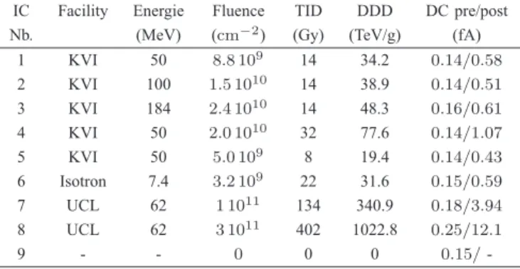
The studied CMOS sensor is a custom 128×128 pixel array with classical three transistors (3T) per pixel design. The pixel pitch is 10μm and the fill factor is about 75 %. This circuit was manufactured in a commercial 0.18μm CMOS technology dedicated to imaging. As described in Tab. II, eight devices were exposed to proton beams at room temperature.
The proton energies range from 7.4 to 184 MeV and the fluences range from5×109to3×1011H+/cm2. Total NIEL values from [12] have been used for displacement damage dose calculation.
After a two month room temperature storage, all the measurements were performed in the dark with temperature regulated to296.15 K. The integration timetintwas kept small enough (between0.1and 0.8 s) to ensure that output voltage variations stay small (< 300 mV) in comparison to readout chain non linearities. If not specified otherwise, the sensors were operated in soft reset mode (see section III-E) to reduce the background noise, the measurement duration was about nine hours and the sampling period about1.6 s. RTS test has not been performed on the devices before their irradiation.
TABLE II
IRRADIATION DETAILS. TIDANDDDDSTAND FOR TOTAL IONIZING DOSE (INGY(SI))AND DISPLACEMENT DAMAGE DOSE RESPECTIVELY. DC PRE/POST MEANS DARK CURRENT MEASURED ON PIXEL ARRAYS BEFORE
AND AFTER PROTON IRRADIATION.
IC Facility Energie Fluence TID DDD DC pre/post
Nb. (MeV) (cm−2) (Gy) (TeV/g) (fA)
1 KVI 50 8.8 109 14 34.2 0.14/0.58
2 KVI 100 1.5 1010 14 38.9 0.14/0.51
3 KVI 184 2.4 1010 14 48.3 0.16/0.61
4 KVI 50 2.0 1010 32 77.6 0.14/1.07
5 KVI 50 5.0 109 8 19.4 0.14/0.43
6 Isotron 7.4 3.2 109 22 31.6 0.15/0.59
7 UCL 62 1 1011 134 340.9 0.18/3.94
8 UCL 62 3 1011 402 1022.8 0.25/12.1
9 - - 0 0 0 0.15/-
For comparison, an additional unirradiated device (IC9) was scanned by the RTS detection code.
In this paper, background noise refers to every temporal noise component except RTS. Therefore, background noise is constituted by readout noise, reset noise and dark current shot noise. The background noise is about0.02 fAfor displacement damage dose below100 TeV/gand reaches0.05 fAin IC7 and 0.12 fAin IC8.
B. Amplitude distributions
In order to correctly interpret the amplitude distributions, it is necessary to model the detection probability Pdt. LetNdt
be the number of detected RTS pixels and Nrts the number of RTS centers in the whole array. The array is constituted by Npix pixels. The detection probability can be defined as Pdt =Ndt/Nrts. A pixel is counted as an RTS pixel if one or more RTS centers with a signal amplitude greater than the minimum detection sensitivityDsvare located in the pixel. In term of probability it means:
Ndt=Npix×P(Arts≥Dsv)×P(nrts≥1), (4) where P(Arts ≥ Dsv) is the probability to have an RTS center with amplitude Arts greater than Dsv, P(nrts ≥ 1) the probability to have one or more RTS defects per pixel andnrtsthe number of RTS defects per pixel. This number is assumed to be governed by the Poisson law:
P(nrts=k) = λke−k
k! , (5)
with λ = Nrts/Npix. Hence, P(nrts ≥ 1) = 1−e−λ. The detection probability is then given by:
Pdt= Ndt
Nrts =P(Arts≥Dsv)×(1−e−λ)
λ . (6)
This probability approaches P(Arts ≥ Dsv) at low fluence when the number of RTS defects is much lower than the number of pixels (i.e. λ→0). It decreases when the number of RTS defects increases and it approaches zero whenλ→ ∞. Therefore, if P(Arts ≥ Dsv) is not close to one the real number of RTS defectsNrtscan not be estimated correctly.
0 0.2 0.4 0.6 0.8 1 1.2 1.4 1.6 1.8 2 100
101 102 103 10
RTS maximum amplitude (fA)
Pixel count
IC9 No irrad.
IC5 19.4 TeV/g IC2 38.9 TeV/g IC4 77.6 TeV/g IC7 340.9 TeV/g IC8 1022.8 TeV/g Exp. fit
Fig. 3. RTS maximum amplitude distributions. Exponential fits of the distribution tails are also presented.
The situation is different if we consider only the number Nrts of RTS defects with maximum amplitude greater than a chosen value Vch. If we choose Vch > Dsv, the probability to detect the RTS defects with amplitude greater than Vch
becomes:
Pdt = Ndt
Nrts = (1−e−λ)
λ , (7)
whereλ=Nrts /Npix. This probability approaches one if the chosenVch is high enough to ensure λ1. In other words, it is possible to find an amplitude above which the number of detected RTS pixels is close to the number of RTS centers (Ndet ≈ Nrts ). On can note that the lower the fluence the lower is this amplitude.
The amplitude distributions of representative ICs are pre- sented in Fig. 3. The extreme amplitude values are no shown for improved clarity but maximum values range from1.5 to 8.5 fAin irradiated devices. The number of pixels presenting RTS behavior in the unirradiated device, about 8%, is quite high compared to previous work but can be partly explain by the use of a more sensitive detection method. About ten per- cent of these RTS pixels were randomly selected and visually checked. All the checked pixel had a real RTS behavior with the same characteristics than proton induced RTS.
Almost all the distributions have a peak shaped part at low amplitude values followed by an exponential tail. Since we have just shown thatNdet ≈Nrts for highest amplitudes RTS, the exponential tail is supposed to represent well the real RTS distribution. This assumption is verified in the next section.
These exponential tails have been fitted by the following exponential function:
F(x) = Nfit
A¯rts
e−x/A¯rts, (8) whereNfit is the total number of RTS centers and A¯rts the mean RTS amplitude. As it can be seen on the distribution slope, this last parameter does not seem to be a function of fluence or proton energy and the mean achieved value is0.19 fA with a 0.03 fA standard deviation. It suggests that a universal maximum amplitude exists for radiation induced RTS, and that its value is about1200±200carrier per second and per RTS center at23◦C. This assumption has to be verified on other devices, other test conditions and especially on a larger number of pixels.
As regards the low amplitude part of Fig. 3, such a peak distribution has not been reported before and the ability of the used method to detect very small RTS fluctuations can explain why. However, we will not study further this part of the distribution in this paper for the following reasons. FirstPdtis too low in this region, and therefore the observed distribution does not correspond to the real RTS defect distribution.
Second, low amplitude RTS are close to the background noise level and we preferred to focus first on higher amplitudes RTS which are the most important from the user point of view.
C. RTS defect counting
Fig. 4 presents three possibilities to count RTS defects.
The most straightforward way is to count the number of detected RTS pixels Ndt. This number does not vary much with irradiation. This can be explained by the fact that when the number of RTS defects increases, Pdt decreases and the resulting number of detected RTS pixels stays almost constant in the displacement damage range used in this paper.
The second RTS population indicator is Nfit, which rep- resents the total number of RTS defects assuming a purely exponential amplitude distribution. In other words, the low amplitude peak is neglected and is supposed to be replaced by an exponential distribution. This implies a significant error on the total number of RTS defects. Nevertheless, Nfit is a good indicator of the most interesting part of the RTS population. One can notice on the figure that Nfit increases linearly with displacement damage dose whatever the proton energy. The same comparison —not presented in this article—
was done with the number of elastic events then with the number of inelastic events. A very poor fit was achieved in both cases for the extreme proton energy values (7.4 MeVand 200 MeV). This suggests that elastic and inelastic interactions both contributes to the RTS center creation process and that this process scales with total NIEL as it was concluded in [5], [9]. The estimated number of RTS defectsNfit generated per displacement damage energy deposited appears to be56.5 RTS centers per (TeV/g) in this pixel array. This corresponds to 46.8 centers· cm−3 · (MeV/g)−1. With the use of the mean amplitude extracted in the previous section, the most interesting part of RTS amplitude distributions can then be predicted using (8).
The same conclusion can be inferred from the number Ndt of detected RTS pixels with amplitudes greater than Vch= 0.5 fA. This number also rises almost linearly (∝x1.1) with displacement damage dose. We chose to count the ampli- tudes above0.5 fAbecause all the distributions are exponential beyond this amplitude. Thus, it can be inferred that for these amplitudes, the number of detected RTS pixels is close to the number of RTS defects. This is confirmed by the high detection probabilityPdt which is close to one in all the tested devices.
D. Number of levels
The distribution of the number of levels detected per pixel is presented in Fig. 5. Multi level RTS can be caused by either
102 103 102
103 104 105
Displacement damage dose (TeV/g)
RTS count Ndt
Nfit N’dt N’fit Y = 2.6 X1.1
Y = 56.5 X
Fig. 4. Evolution of the number of RTS defects with displacement damage dose.Ndtis the total number of detected RTS pixels,Nfitthe total number of RTS defects estimated with the exponential fit,Ndt the number of detected RTS pixels with amplitude greater than0.5 fAandNfit the estimated number of RTS defects with maximum amplitude greater than0.5 fA.
0 2 3 4 5 6 7 8 9 10
100 101 102 103 104
Number of levels
Pixel count
IC9 No irrad.
IC5 19.4 TeV/g IC2 38.9 TeV/g IC4 77.6 TeV/g IC7 340.9 TeV/g IC8 1022.8 TeV/g
Fig. 5. Distribution of the number of RTS levels in IC9, IC5, IC2, IC4, IC7 and IC8. IC1, IC2, IC3 and IC6 received similar displacement damage doses and have approximately the same RTS level distribution. For improved clarity, only IC3 is shown to represents these distributions.
a sum of two or more 2-level RTS centers, one or more multi- level RTS centers or the combination of both [5]. If the sum of independent 2-level RTS center hypothesis is considered, the observed number of levels should only be equal to powers of two [1]. It will then be assumed that a number of levelsNlvl that does not correspond to a power of two is in fact equal to the closest power of two greater than Nlvl. The missing levels are assumed to be missed during the level counting process. Therefore, the number of pixels withn defects per pixelNpix(Ndef =n)is retrieved from the number of pixels withk levels per pixelNpix(Nlvl=k)thanks to:
Npix(Ndef =n) =
2n
k=1+2(n−1)
Npix(Nlvl=k). (9) The resulting distribution is compared to a Poisson distribution with λ = 0.1 in Fig. 6. The Poisson distribution has been multiplied by the total number of pixels to be compared with the measurements. Both distributions match quite well. This clearly shows that the independent 2-level RTS center theory can explain the multi level RTS observed on the unirradiated device.
We tried to use the same approach on irradiated devices.
However the probability to have 2-level RTS pixels in com- parison to more than 2-level RTS pixels is very high and
0 1 2 3
100 101 102 103 104
Number of defects per pixel
Pixel count
IC9 No irrad.
Npix× Poisson{λ = 0.1}
Fig. 6. Distribution of the number of defects per pixel compared to the Poisson distribution with λ = 0.1. The number of defects per pixel is estimated from the number of level distribution thanks to (9)
can not be explained by a Poisson law. The fluences are supposed too high to correctly detect all the RTS levels.
The radiation induced noise is supposed to reduce the level detection efficiency and change the distribution shape. This is confirmed by the decrease of the number pixels with more than two levels observed in Fig. 5 when the displacement damage dose increases. This suggests that the number of multi level RTS, in comparison to 2-level RTS, should be greater than what is observed.
E. Photodiode bias effect
In order to see the influence of applied electric field on RTS behavior, dark current fluctuations were measured during one hour at several photodiode reverse biases. During reset, photodiode cathode voltage can be adjusted by changing the reset voltageVRST. This is only true in hard reset mode. This operating mode [13] corresponds toVG−VRST> VthwithVG
andVth the reset transistor gate voltage and threshold voltage respectively. On the contrary, in soft reset mode whenVRST>
VG−Vth, the photodiode cathode voltage is pinned toVG−Vth at the end of the reset phase. In this device, the transition between hard and soft reset was found to be close to 2.4 V.
Therefore, forVRSTgreater than2.4 Vthe photodiode is reset to 2.4 V. Otherwise the photodiode is reset toVRST.
The following reset transistor drain voltages VRST have been used: 3.3 V,2.4 V,2.0 Vand1.6 Vwith sampling time set to 1.12 s. The mean cathode voltage variation during integration was kept small (≈ 20 mV) in comparison to the voltage step used.
The result of this test is illustrated in Fig 7. This figure shows the dark current evolution with time of a representative four-level RTS pixel for the four selected biasing conditions.
As expected [14], we can see that the background noise almost double from soft to hard reset mode. However, the other RTS characteristics (amplitudes and time constants) remain unchanged. This is not surprising since the photodiode voltage after a soft reset is close to 2.4 V. When the reset voltage, which is equal to the cathode voltage in hard reset, decreases from2.4 Vto1.6 Vthe mean dark current also decreases. This is obviously caused by the depletion region reduction which is known to decrease PN junction generation current.
As regards the RTS amplitudes, it is quite surprising to notice that it is not affected by the applied voltage. Indeed, the most suggested cause of RTS large amplitude is electric
0 50 100 150 200 1
1.5 2 2.5 3
Time (mn)
Dark current (fA)
VRST = 3.3V (SRst) V
RST = 2.4V (HRst) V
RST = 2.0V (HRst) V
RST = 1.6V (HRst)
Fig. 7. 4-level RTS measured at 4 different reset conditions. This response was extracted from an IC4 pixel. SRst stands for soft reset and Hrst for hard reset.
0 0.2 0.4 0.6 0.8 1 1.2 1.4
100 101 102 103
Amplitude (fA)
Pixel count
VRST = 3.3V VRST = 2.4 V VRST = 2.0 V VRST = 1.6 V
Fig. 8. Evolution of RTS amplitude distribution with reset voltage.
field enhancement [1], [4], [6]. Since applied electric field is assumed to decrease with external voltage, and since electric field enhancement is an exponential process, RTS amplitude should dramatically be reduced by a voltage decrease.
The same trends can be observed on every RTS pixels.
Fig. 8 presents the RTS amplitude distributions. As expected from the previous conclusion, no significant change can be seen on the distributions for amplitude greater than 0.1 fA where P(Arts ≥ Dsv) ≈ 1. Nevertheless, a lot more of weak transitions (<0.1 fA) are detected in the soft reset mode because the background noise is reduced andP(Arts≥Dsv) increased.
The fact that applied voltage does not seem to have any in- fluence on RTS amplitudes strongly suggests that electric field enhancement is not the main cause of large RTS amplitudes.
This supports the findings of Bogaertset al.[4] who mentioned inter-center charge transfer [15] as a possible explanation for high RTS amplitudes. However, as discussed in [9], a defect which can induce charge exchange reaction and that exhibits a switching behavior still has to be identified. Enhancement due to defect local electric field could be an alternative explanation but such electric field is also supposed to be a function of reverse bias [16].
IV. SUMMARY AND CONCLUSION
A new detection method able to automatically extract multi level RTS parameters has been proposed. This method appears to be an efficient tool for studying a large number of RTS pixels. The first results achieved with this technique indicate that RTS maximum amplitude distributions can be divided in two parts. A peak shaped at low amplitude, which will
be studied in future work and an exponential tail for larger amplitudes. The exponential fit of this tail gave a universal RTS maximum amplitude of about 0.19 fAper RTS center at 23◦C. A number of defects has also been extracted and appears to increase linearly with displacement damage dose with the following factor: 46.8 centers·cm−3·(MeV/g)−1. Thanks to these two parameters, RTS amplitude distributions can be predicted. The fluences used in this study seem too high to produce optimum RTS level distributions and lower fluences will be used in future studies. The effect of applied electric field, through the variation of photodiode reset voltage, has also been studied. As expected, the decrease of bias voltage reduced the mean dark current generation through a depletion region reduction. However, no change in RTS amplitude was observed. This suggests that electric field enhancement does not play an important role in the RTS center generation enhancement.
REFERENCES
[1] I. H. Hopkins and G. R. Hopkinson, “Random telegraph signals from proton-irradiated CCDs,” IEEE Trans. Nucl. Sci., vol. 40, no. 6, pp.
1567–1574, Dec. 1993.
[2] ——, “Further measurements of random telegraph signals in proton- irradiated CCDs,”IEEE Trans. Nucl. Sci., vol. 42, no. 6, pp. 2074–2081, Dec. 1995.
[3] G. R. Hopkinson, “Radiation effects in a CMOS active pixel sensor,”
IEEE Trans. Nucl. Sci., vol. 47, no. 6, pp. 2480–2484, Dec. 2000.
[4] J. Bogaerts, B. Dierickx, and R. Mertens, “Random telegraph signal in a radiation-hardened CMOS active pixel sensor,”IEEE Trans. Nucl. Sci., vol. 49, no. 1, pp. 249–257, Feb. 2002.
[5] A. M. Chugg, R. Jones, M. J. Moutrie, J. R. Armstrong, D. B. S. King, and N. Moreau, “Single particle dark current spikes induced in CCDs by high energy neutrons,”IEEE Trans. Nucl. Sci., vol. 50, no. 6, pp.
2011–2017, Dec. 2003.
[6] D. R. Smith, A. D. Holland, and I. B. Hutchinson, “Random telegraph signals in charge coupled devices,”Nucl. Instr. and Meth. A, vol. 530, no. 3, pp. 521–535, Sep. 2004.
[7] T. Nuns, G. Quadri, J.-P. David, O. Gilard, and N. Boudou, “Measure- ments of random telegraph signal in CCDs irradiated with protons and neutrons,”IEEE Trans. Nucl. Sci., vol. 53, no. 4, pp. 1764–1771, Aug.
2006.
[8] T. Nuns, G. Quadri, J.-P. David, and O. Gilard, “Annealing of Proton- Induced Random Telegraph Signal in CCDs,”IEEE Trans. Nucl. Sci., vol. 54, no. 4, pp. 1120–1128, Aug. 2007.
[9] G. R. Hopkinson, V. Goiffon, and A. Mohammadzadeh, “Random telegraph signals in proton irradiated CCDs and APS,” inIEEE Trans.
Nucl. Sci., vol. 55, no. 4, Aug. 2008.
[10] Y. Yuzhelevski, M. Yuzhelevski, and G. Jung, “Random telegraph noise analysis in time domain,”Rev. Sci. Instr., vol. 71, no. 4, pp. 1681–1688, Apr. 2000.
[11] A. Konczakowska, J. Cichosz, and A. Szewczyk, “A new method for RTS noise of semiconductor devices identification,” IEEE Trans.
Instrum. Meas., vol. 57, no. 6, pp. 1199–1206, Jun. 2008.
[12] C. J. Dale, L. Chen, P. J. McNulty, P. W. Marshall, and E. A. Burke,
“A comparison of monte carlo and analytical treatments of displacement damage in Si microvolumes,”IEEE Trans. Nucl. Sci., vol. 41, no. 6, pp.
1974–1983, Dec. 1994.
[13] B. Pain, G. Yang, T. Cunningham, C. Wrigley, and B. Hancock, “An enhanced-performance CMOS imager with a flushed-reset photodiode pixel,”IEEE Trans. Electron Devices, vol. 50, no. 1, pp. 48–56, Jan.
2003.
[14] H. Tian, B. Fowler, and A. Gamal, “Analysis of temporal noise in CMOS photodiode active pixel sensor,”IEEE J. Solid-State Circuits, vol. 36, no. 1, pp. 92–101, Jan. 2001.
[15] S. Watts, J. Matheson, I. Hopkins-Bond, A. Holmes-Siedle, A. Moham- madzadeh, and R. Pace, “A new model for generation-recombination in silicon depletion regions after neutron irradiation,”IEEE Trans. Nucl.
Sci., vol. 43, no. 6, pp. 2587–2594, Dec. 1996.
[16] A. Czerwinski, “Defect-related local-electric-field impact on p–n junc- tion parameters,”Appl. Phys. Lett., vol. 75, no. 25, pp. 3971–3973, 1999.