HAL Id: hal-01491829
https://hal.archives-ouvertes.fr/hal-01491829
Submitted on 17 Mar 2017
HAL is a multi-disciplinary open access
archive for the deposit and dissemination of sci-entific research documents, whether they are pub-lished or not. The documents may come from teaching and research institutions in France or abroad, or from public or private research centers.
L’archive ouverte pluridisciplinaire HAL, est destinée au dépôt et à la diffusion de documents scientifiques de niveau recherche, publiés ou non, émanant des établissements d’enseignement et de recherche français ou étrangers, des laboratoires publics ou privés.
Factors influencing prokaryotes in an intertidal mudflat
and the resulting depth gradients
Céline Lavergne, Hélène Agogué, Aude Leynaert, Mélanie Raimonet, Rutger
de Wit, Philippe Pineau, Martine Bréret, Nicolas Lachaussée, Christine
Dupuy
To cite this version:
Céline Lavergne, Hélène Agogué, Aude Leynaert, Mélanie Raimonet, Rutger de Wit, et al.. Factors influencing prokaryotes in an intertidal mudflat and the resulting depth gradients. Estuarine, Coastal and Shelf Science, Elsevier, 2017, 189, pp.74 - 83. �10.1016/j.ecss.2017.03.008�. �hal-01491829�
1
Factors influencing prokaryotes in an intertidal mudflat
1and the resulting depth gradients
23
Céline Lavergne * 1,4, Hélène Agogué 1, Aude Leynaert 2, Mélanie Raimonet 2, Rutger 4
De Wit 3, Philippe Pineau 1, Martine Bréret 1, Nicolas Lachaussée 1, Christine Dupuy 1 5
6
1 LIENSs, UMR 7266 Université de la Rochelle, CNRS. 2 rue Olympe de Gouges, 17000 La 7
Rochelle, France 8
2 LEMAR, UMR 6539 Université de Bretagne Occidentale, CNRS, IRD, Ifremer. Institut 9
Universitaire Européen de la Mer, 29280 Plouzané, France 10
3 Center for Marine Biodiversity, Exploitation and Conservation (MARBEC). Université de 11
Montpellier, CNRS, IRD, Ifremer. Place Eugène Bataillon, Case 093, F-34095 Montpellier 12
Cedex 5, France 13
4 School of Biochemical Engineering, Pontificia Universidad Católica de Valparaíso, Avenida 14
Brasil 2085, Valparaíso, Chile 15
*Corresponding author: Céline Lavergne, School of Biochemical Engineering,
16
Pontificia Universidad Católica de Valparaíso, Avenida Brasil 2085, Valparaíso, Chile 17
e-mail: lavergne.celine@gmail.com 18
19
Running title: Prokaryote drivers in mudflats 20
2
1 Highlights
21
Strong stratification in two horizons of microbial densities and activities in the first 22
10 cm of the sediment. 23
A gradual transition could correspond to an environmental ecocline rather than an 24
ecotone. 25
Bottom-up-control of the prokaryotic community revealed by the variation partitioning 26 analysis.27 28
2 Abstract
29Intertidal mudflats are rich and fluctuating systems. The upper 20 cm support a high 30
diversity and density of microorganisms that ensure diversified roles. The depth profiles of 31
microbial abundances and activities were measured in an intertidal mudflat (Marennes-Oléron 32
Bay, SW France) at centimeter-scale resolution (0-10 cm below the sediment surface). The aim 33
of the study was to detect microbial stratification patterns within the sediments and how this 34
stratification is shaped by environmental drivers. Two sampling dates, i.e. one in summer and 35
another in winter, were compared. The highest activities of the microbial communities were 36
observed in July in the surface layers (0-1 cm), with a strong decrease of activities with depth. 37
In contrast, in February, low microbial bulk activities were recorded throughout the sediment. 38
In general, prokaryotic abundances and activities were significantly correlated. Variation 39
partitioning analysis suggested a low impact of predation and a mainly bottom-up-controlled 40
prokaryotic community. Hence, in the top layer from the surface to 1–3.5 cm depth, microbial 41
communities were mainly affected by physicochemical variables (i.e., salinity, phosphate and 42
silicate concentrations). Below this zone and at least to 10 cm depth, environmental variables 43
were more stable and prokaryotic activities were low. The transition zone between both layers 44
probably represents a rather smooth gradient (environmental ecocline). The results of our study 45
provide a better understanding of the complex interactions between micro-organisms and their 46
environment in a fluctuating ecosystem such as an intertidal mudflat. 47
Keywords: intertidal mudflat, sediment depth, microbial communities, benthic ecology
3
3 Introduction
49
In temperate zones, intertidal mudflats are among the most productive coastal 50
ecosystems due to the development of an active microphytobenthic biofilm at the surface of the 51
sediment (Admiraal, 1984; Underwood and Kromkamp, 1999). Several factors drive the high 52
productivity levels such as incident light and large nitrogen-rich inputs from the continent 53
(Underwood and Kromkamp, 1999), in these complex ecosystems. The knowledge about the 54
relationship between the microphytobenthos and the activity of prokaryotic communities, 55
although recognized as of paramount importance for determining the productivity of these 56
ecosystems (Agogué et al., 2014; Decho, 2000; McKew et al., 2013; Orvain et al., 2014a), is 57
still largely insufficient (Van Colen et al., 2014). Marine coastal sediments harbor among the 58
most diverse and abundant prokaryotic communities (Whitman et al., 1998; Zinger et al., 2011). 59
The abundances and activities of these microbial communities seem to vary along a vertical 60
gradient at a restricted vertical scale (e.g., < 20 cm) under the influence of the 1) organic matter 61
composition and quality and electron acceptor availability (Kristensen, 2000), 2) physical 62
properties of the sediments, 3) bioturbation and bioirrigation activities 4) bottom-up and top-63
down trophic controls, and 5) climatic conditions. 64
The dominant source of carbon for heterotrophic microorganisms in temperate intertidal 65
mudflats is derived from microphytobenthic activities (i.e., photosynthesis and exopolymeric 66
substance production) (Underwood and Kromkamp, 1999). This organic matter production is 67
primarily ensured by epipelic (i.e., motile free-living) diatoms and quickly transferred to other 68
biological compartments (Middelburg et al., 2000). The microphytobenthic biofilm has such a 69
relevant effect on prokaryotic communities at low tide that it drastically modifies the 70
remineralization and fluxes of inorganic nutrients across the sediment surface (Middelburg et 71
al., 2000). 72
4
In muddy fine-grained low-permeable sediments, where advection fluxes are almost 73
absent, physical transport of solutes is mainly driven by molecular diffusion within the 74
interstitial water. The top sediment layers show a strong consumption of oxygen by 75
organotrophic microorganisms and by reoxidation of reduced compounds such as Fe2+, Mn2+, 76
H2S (Soetaert et al., 1996). Hence, oxygen does not diffuse below the first few millimeters in 77
mudflats where deeper sediment are most often anoxic (Bertics and Ziebis, 2010). Other 78
inorganic electron acceptors, including the nutrient nitrate, can thus be used deeper in the 79
sediment by dissimilatory processes (e.g., denitrification) for anaerobic mineralization. Hence, 80
microbial communities may exhibit vertical patterns in the nature and rate of their activity in 81
response to changing biogeochemical conditions, implicating different prokaryotic assemblage. 82
Moreover, infauna activity plays a crucial role in the modulation of microbial activity 83
in sediments by disturbing the vertical gradients of oxygen, organic matter and inorganic 84
nutrients (Bertics and Ziebis, 2009; Gilbertson et al., 2012; Jones et al., 1996). As an example, 85
prokaryotic activity has been shown to be increased by both bioirrigation and bioturbation 86
activities in a coastal lagoon of the Santa Catalina Island (CA, USA) (Bertics and Ziebis, 2009). 87
Furthermore, prokaryotes may strongly vary under trophic controls. The impact of the 88
availability of resources (e.g., organic matter and/or inorganic nutrients) is defined as the 89
bottom-up control of the microbial communities (Fuhrman and Hagström, 2008), and may 90
strongly change at both spatial and temporal scales. On the other hand, top-down control is 91
described as grazing pressure primarily carried out by meiofauna or viruses (i.e., prokaryotic 92
cell lysis) in intertidal mudflats. Among the few studies focusing on the balance of bottom-93
up/top-down control in mudflats, the role of top-down control by meiofauna seems to be 94
significant and could be more important than bottom-up control (Fabiano and Danovaro, 1998), 95
although a local study indicated that grazing pressure did not represent a crucial control of 96
bacterial community (Pascal et al., 2009). In a microcosm study, De Mesel et al. (2004) 97
5
highlighted that both trophic controls have to be considered as bacterial community structure is 98
a function of substrate but the relative abundance of each taxa is influenced by the grazing 99
activities of bacterivorous nematods. 100
Finally, in intertidal zones and especially in macrotidal systems, the alternation of 101
emersion and immersion produces drastically fluctuating conditions, particularly during low 102
tide at the sediment surface. For example, temperature, a key factor impacting prokaryotic 103
metabolism in coastal sediments (Hubas et al., 2007), can fluctuate significantly within 6 hours 104
of a low tide (until 16°C of amplitude measured at the sediment surface in the Marennes Oléron 105
mudflat, France, Orvain et al. (2014a)). Moreover, in these shallow ecosystems, other climatic 106
conditions such as wind or waves can strongly disturb the global (i.e., biotic and abiotic) vertical 107
zonation of the sediment (Dupuy et al., 2014). 108
The aims of this study were 1) to describe stratification patterns of the activities and 109
densities of prokaryotic communities in coastal mudflats at cm-scale spatial resolution and 2) to 110
statistically disentangle the relative contributions of environmental variables and meiofauna 111
abundances in the different depth layers as possible drivers for these prokaryotic activities and 112
densities. This work was focused on an intertidal mudflat in Marennes-Oléron Bay (SW France) 113
sampled twice at low tide, during representative summer and winter conditions, respectively in 114
assessed how the patterns of prokaryotic densities and activities varied with depth and to 115
identify the impact of physicochemical variables and potential grazing pressure on the 116
stratification observed. 117
6
4 Materials and Methods
118
4.1 Study site and sampling
119
Sediment cores were sampled in Marennes-Oléron Bay on the Atlantic French coast (1 km 120
from the shore) (N 45° 54ʹ 53ʺ; W 01° 05ʹ 23ʺ). The intertidal mudflat is characterized by the 121
presence of parallel ridges and runnels and sampling was performed on ridges at low tide. Two 122
sampling dates were compared at a similar tidal range (5.5 ± 0.2 m): 1) on July 5, 2012, high 123
temperature and incident irradiance and 2) on February 11, 2013, low temperature and incident 124
irradiance. 125
On each sampling date, triplicate 15-cm diameter cores were sliced in situ into five layers 126
using a piston inserted below the core from 0 to 10 cm below the sediment surface (bsf) (D1 = 127
0-0.5 cm; D2 = 0.5-1 cm; D3 = 1-2 cm; D4 = 2-5 cm and D5 = 5-10 cm). Samples were 128
homogenized and subdivided using 50-ml sterile syringes with cut-off tips for further analysis 129
(storage conditions differed according to the variable, see Supp info Table S1). Triplicate cores 130
12-cm in diameter were simultaneously recovered for the determination of pore-water nutrient 131
concentrations. These cores were pre-drilled vertically at 0.5 cm resolution, and pore water was 132
collected at 0.5, 1, 1.5, 3.5 and 7.5 cm bsf, using the Rhizons® (Rhizosphere Research Products 133
Netherlands ) method (Seeberg-Elverfeldt et al., 2005). The Rhizons were inserted horizontally 134
into the sediment core during 20 minutes to collect enough pore-water volume for subsequent 135
analysis. 136
4.2 Physical and chemical analysis
137
Incident irradiance and temperature at the surface of the sediment were assessed in situ 138
every 30 seconds with a universal light-meter and data logger (ULM-500, Walz Effeltrich, 139
Germany) equipped with a plane light/temperature sensor (accessory of the ULM-500) and a 140
plane cosine quantum sensor (Li-COR, USA). Depth temperature profiles were measured every 141
7
30 seconds during all the sampling period with five 3.1-cm length Hobo sensors (Hobo Pro V2, 142
USA) fixed on a homemade stick that was vertically pushed into the sediment to position the 143
sensors at 5 different depths (0.5 cm, 1 cm, 2 cm, 5 cm and 10 cm bsf). 144
At the laboratory, pore-water pH and salinity (using the Practical Salinity Scale) were 145
measured in the supernatant after centrifugation (15 min, 3,000 ×g at 8 °C) with a pH probe 146
(Eutech Instruments PC150, USA) and a conductivity meter (Cond 3110, TetraCon 325, WTW, 147
Germany), respectively. Sediment density and porosity were evaluated by weighing 50 ml of 148
fresh sediment before and after drying (48 h at 60 °C). Porosity was calculated as the ratio of 149
the volume of water divided by the total volume of sediment. After removal of salts and organic 150
matter, the mean grain size of the sediment was measured by a laser granulometer (Mastersizer 151
2000, Malvern Instruments, U.K.) and evaluated using the GRADISTAT program (Blott and 152
Pye, 2001) according to the Folk and Ward theory (Folk and Ward, 1957). 153
Total organic carbon (TOC) and total nitrogen (TN) contents were measured on 154
lyophilized samples by oxic combustion at 950°C (Strickland and Parsons, 1972) using a CHN 155
elemental analyzer (Thermo Fisher Flash EA 1112, Waltham, MA, USA). Samples for TOC 156
were decarbonated (in hydrochloric acid, HCl 1N) prior to combustion to remove the inorganic 157
carbon. Because the decarbonation could biased the TN content analysis, subsamples were ran 158
before and after decarbonation to validate the TN measurement. 159
Two exopolymeric (EPS) fractions (colloidal and bound) were extracted in two steps: 160
colloidal EPS were extracted using fresh sediment mixed with an equal volume of artificial 161
seawater, then bound EPS were extracted using the residual sediment mixed with Dowex resin 162
(Takahashi et al., 2009). Before quantification of EPS-proteins and -carbohydrates, each extract 163
was vacuum-evaporated over 6h (Maxi Dry plus, Heto, Denmark). Colloidal and bound EPS-164
protein concentrations were determined using the bicinchoninic acid assay (Smith et al., 1985). 165
Colloidal and bound EPS-carbohydrate concentrations were determined according to the 166
8
phenol-sulfuric acid method (Dubois et al., 1956). The four resulting fractions colloidal EPS-167
proteins, bound EPS-proteins, colloidal EPS-carbohydrates and bound EPS-carbohydrates were 168
expressed in µg g-1 sed DW. Colloidal EPS correspond to the sum of colloidal EPS-proteins 169
and colloidal EPS-carbohydrates. Bound EPS correspond to the sum of bound EPS-proteins 170
and bound EPS-carbohydrates. Colloidal EPS and bound EPS were used for the calculation of 171
the ratio colloidal EPS / bound EPS. EPS-carbohydrates correspond to the sum of colloidal 172
EPS-carbohydrates and bound EPS-carbohydrates. EPS-proteins correspond to the sum of 173
colloidal EPS-proteins, bound EPS-proteins. EPS-carbohydrates and EPS-proteins were used 174
for the calculation of the ratio EPS-carbohydrates/EPS-protein. 175
Total protein content was determined in sediment (stored at -20 °C) after extraction (30 176
min, in the dark, +4 °C in 0.2-µm-filtered seawater) using Lowry Peterson’s modification assay 177
(Sigma-Aldrich). Ammonium (NH4+), nitrites (NO2-), nitrates (NO3-), phosphate (PO43-), and 178
silicate (Si(OH)4) concentrations were determined using an autoanalyzer (Seal Analytical, 179
GmbH Nordertedt, Germany) equipped with an XY-2 sampler according to Aminot and 180
Kérouel (2007). 181
4.3 Biotic parameters
182
Chlorophyll a, used as a proxy of algal biomass, was assessed by fluorimetry (640 nm, 183
Turner TD 700, Turner Designs, USA) after extraction with 90% acetone. Chlorophyll a 184
concentrations were expressed as µg g-1 sediment dry weight (DW) according to Lorenzen 185
(1966). Prokaryotic abundance was evaluated by flow cytometry after a cell extraction 186
procedure described by Lavergne et al. (2014). 187
Analyses of the two potential extracellular enzymatic activities, β-glucosidase and 188
aminopeptidase, were determined by spectrofluorimetry (Boetius, 1995) (SAFAS Scientific 189
Instruments, Monaco) [excitation/emission = β-glucosidase activity: 365 nm/460 nm; and 190
9
aminopeptidase: 340 nm/410 nm]. For β-glucosidase activity, slurry sediment samples were 191
incubated in triplicate using 4-Methylumbelliferyl β-D-glucopyranoside (500 µmol L-1 final 192
conc.) as a substrate at three different incubation times: 15, 45, and 75 min. For aminopeptidase 193
activity, slurry sediment samples were incubated in triplicate with L-leucine β-naphthylamide 194
hydrochloride (300 µmol L-1, final conc.) as a substrate at three different incubation times: 10, 195
30, and 60 min. Final concentrations of 4-Methylumbelliferyl β-D-glucopyranoside and L-196
leucine β-naphthylamide hydrochloride were determined previously to represent saturation 197
levels and maximum yield velocities (Vmax) (Boetius and Lochte, 1996). 198
Incorporation of [methyl-3H] thymidine into DNA was measured as a proxy of benthic 199
bacterial production (Garet and Moriarty, 1996; Pascal et al., 2009). Briefly, 30 µl of fresh 200
sediment slurry (vol/vol; 0.2-µm-filtered seawater) was incubated with 3H-thymidine 0.74 201
106 Bq for 1 h at in situ temperature (22°C in July and 12°C in February). Blank controls were 202
stopped just after the addition of labelled 3H-thymidine with 8 ml of cold 80% ethanol. After 203
incubation, samples were stopped with 8 ml of cold ethanol (80%). After two washes with 80% 204
cold ethanol by mixing and centrifugation (15 min, 4 500 g, +4°C), slurries were transferred 205
with 2 mL of ice-cold TCA (5%, trichloroacetic acid) onto a polycarbonate filter (Nuclepore 206
0.2 µm, 25 mm, Millipore, NJ, USA). Subsequently, the filters were washed four times with 207
5% ice-cold TCA. Afterwards, the filters were transferred into scintillation vials containing 2 208
ml 0.5N chlorhydric acid and incubated 16 h at +95°C (Garet and Moriarty, 1996). Supernatant 209
(0.5 mL) was transferred in a new scintillation vial with 5 mL of scintillation fluid (Ultima 210
Gold, Perkin-Elmer, MA, USA). The amount of radioactivity in each vial was measured using 211
a scintillation counter (Perkin-Elmer, USA). Benthic bacterial production was finally expressed 212
as pmol 3H Thy g-1 sed DW h-1 using a conversion factor 4.51 10-13 (Ci dpm-1) evaluated 213
experimentally to account for counter efficiency. 214
10
For meiofaunal assemblage determination, samples from each depth (60 mL) were 215
stored directly after sampling at room temperature in absolute ethanol, sieved through 50 µm 216
before staining with rose Bengal and observation under stereo microscope (Zeiss). Foraminifera 217
were counted in all the sediment samples, and for other meiofauna organisms (i.e., juvenile 218
gastropods, copepods, ostracods, nematods, foraminifera, and juvenile bivalves), samples were 219
diluted prior to counting. Abundances were expressed as individuals (ind.) per cm3. 220
Additionally, six 20-cm diameter PVC cores were harvested at each date and sieved through 1 221
mm. The macrofauna was collected and stored in ethanol 60% for further identification. In the 222
current study, only the data of the abundance of the macrozoobenthic grazer, Peringia ulvae 223
(Pennant, 1777) are presented. The mean abundance of the six cores is expressed in ind m-2. 224
4.4 Statistical analyses
225
All statistical analyses were performed with R software (R Core Team, 2013). In this 226
study, the results are presented as the means ± standard error (SE) because the SE evaluates the 227
mean estimation imprecision. To evaluate the effect of temperature on thymidine incorporation 228
rate, Q10 values were calculated at each sampling depth (Lomas et al., 2002) using the Equation 229
1. 230
Equation 1: 𝑄10= (𝑅2 𝑅1⁄ )(10 𝑡⁄2−𝑡1) 231
Where R2 and R1 are the thymidine incorporation rates and t2 and t1 are the incubation
232
temperatures in July and February, respectively. This factor indicating the increase of a process 233
rate with 10°C increase of temperature is more powerful when calculated with large dataset 234
and/or used with regression data (Hubas et al., 2007; Lomas et al., 2002). In the current study, 235
as the replicates are independent between the two sampling dates, Q10 factor was calculated for 236
11
all the possible combinations (n=33). Then, a student test for one sample was used to evaluate 237
whether the Q10 values were significantly different from 1. 238
Pearson tests were used to test whether the distribution of two variables was similar. 239
The significant variation of environmental and prokaryotic variables among sediment depths 240
and sampling dates was evaluated by two-way ANOVA (using sampling date - 2 levels - and 241
depths - 5 levels - as factors) followed by multiple comparison tests (Tukey HSD test) and 242
variance homogeneity and residuals normality were tested. For the two variables “chlorophyll 243
a” and “Q10 of thymidine incorporation”, the ANOVA assumptions were violated, the variables 244
were ln-transformed and two-way ANOVA followed by Tukey HSD test was performed. For 245
the two variables “EPS-carbohydrates/EPS-protein” and “colloidal EPS/ bound EPS”, the 246
ANOVA assumptions were violated and transformation was not possible, non-parametric 247
Friedman test was thus run followed by the Nemenyi post-hoc test for multiple joint samples 248
(Nemenyi, 1963; Sachs, 1997) using the “PMCMR” package (Pohlert, 2014). 249
Multivariate principal component analysis (PCA) was performed for July sampling and 250
February sampling separately with 8 environmental variables using the “FactoMineR” package 251
(Husson et al., 2013). Then, in order to define sediment horizons using the basis of each PCA 252
obtained, a hierarchical clustering analysis was applied using the HCPC function of the 253
“FactoMineR” package (Husson et al., 2013). 254
Finally, in order to disentangle the impacts of the environmental variables and 255
meiofaunal group abundance, both taken individually as well as shared, on the distribution of 256
prokaryotic density and activities, variation partitioning was performed (Borcard et al., 1992; 257
Ramette, 2007; Volis et al., 2011) using the varpart function of the “vegan” packages (Oksanen 258
et al., 2013)). First, one response table and three explanatory tables were built and composed 259
as follows. The response table corresponds to the “prokaryotic” table (P table) containing 260
prokaryotic abundance (PA), thymidine incorporation (Thy.inc), aminopeptidase activity 261
12
(AMA), and β-glucosidase activity (BGA) and was standardized to unit variance. The 262
explanatory “meiofauna” table (M table) containing abundances of juvenile gastropods, 263
copepods, ostracods, nematods, foraminifera, and juvenile bivalves was log10(x + 1) 264
transformed to normalize the distribution. And the explanatory table of the “environmental 265
variables” (E table) (standardized) contains temperature, salinity, pH, the ratio DIN:PO43-, the 266
ratio TOC:TN, total protein content, porosity, EPS-carbohydrates/EPS-protein and colloidal 267
EPS/bound EPS. 268
Using forward selection procedure (Legendre and Legrendre, 1998) with the function 269
forward.sel in the package ‘packfor’ (Dray et al., 2013), we selected the variables that 270
influenced the most the response table (Ramette and Tiedje, 2007). The final explanatory tables 271
was thus composed as follows: the table E containing phosphate and silicate concentrations as 272
well as salinity and the table M containing abundance of juvenile gasteropods. The variation 273
partitioning evaluates diverse components of variation of a set of response variables: 1) the pure 274
effect of each individual explanatory table without the effect of the other explanatory table; 2) 275
the redundancy of the two explanatory tables which is the part of the variance explained by both 276
explanatory tables; and 3) the residual effects unexplained by the chosen variables (Borcard et 277
al., 1992; Volis et al., 2011). In this set of data, it is expected that the distribution of abundances 278
and activities of prokaryotes (P table) responds linearly to the explanatory variables, thus we 279
used the linear-based PCA and redundancy analysis (RDA) for the analysis. The total variance 280
to be explained was evaluated by a PCA with the abundances and activities of prokaryotes (P 281
table). RDA was used to assess the amount of variation of the P table explained by the two 282
explanatory variables (as constraining variables). Using partial RDA (pRDA), the effect of a 283
set of variable (an explanatory table) could be removed from the analysis if selected as a 284
covariable. This is an important issue of this multivariate analysis that, in the present case, 285
evaluates for example the effect of meiofauna on prokaryotic variables without the effect of the 286
13
environmental variables. These environmental variables such as salinity could indeed be 287
important factors for both prokaryotic and meiofaunal communities and the partition of these 288
effects allows to quantify the pure effect of the meiofauna without the shared variation with 289
environmental variables. Finally, the significance of each ordination was tested by an ANOVA 290
like permutation test using 9999 permutations (Volis et al., 2011). 291
5 Results
292
5.1 Environmental conditions and variation of physicochemical variables
293
The air temperature and incident irradiance at the surface of the mudflat were 28 ± 294
0.9 °C and 1800 ± 156 µmol photons m-2 s-1 and 10.5 ± 1.1 °C and 611 ± 292 µmol photons m -295
2 s-1 during the samplings in July and in February, respectively (Supp info Fig. S1 and Table 296
S2). The sediment was predominantly silt-clay (mean of 91.2%), with an average grain size of 297
11.17 ± 0.34 µm and a porosity of 0.73 ± 0.01. 298
Two-way ANOVA reveals that all the physicochemical variables (presented in the Table 299
1) were significantly different between the two sampling dates (p < 0.05) except the Colloidal 300
EPS / bound EPS ratio. Significant variations with sediment depth are highlighted by Tukey’s 301
post hoc test (Table 1, see Supp info Fig. S2 to Fig. S4 for detailed profiles). 302
Then, two principal component analysis (PCA) were performed using 8 variables (i.e., 303
presented in the Table 1 except grain size, porosity and algal biomass) aiming at describing the 304
interactions within the physicochemical variables for each sampling date and a hierarchical 305
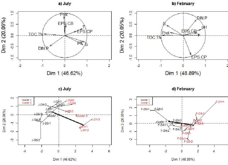
clustering analysis based on the ordinations obtained was used to group the samples. In July, 306
the two first dimensions of the PCA together explained 66.68 % of the observed variability in 307
the dataset (Figure 1a). The first dimension was mostly characterized by TOC:TN, pH, salinity 308
and temperature and differentiated the samples in two groups from 0 to 1 cm bsf on one hand 309
14
and the samples from 1 to 10 cm bsf on the other hand (Figure 1c). In February, the two first 310
dimensions of the PCA together explained 68.94 % of the observed variability in the dataset 311
(Figure 1b). The first dimension was mostly characterized by TOC:TN, pH and temperature 312
and differentiated the samples in two groups from 0 to 2 cm bsf on one hand and the samples 313
from 2 to 10 cm bsf on the other hand (Figure 1d). 314
In both cases, DIN:PO43- and EPS-carbohydrates/EPS-proteins ratios have information 315
represented in both dimensions of the ordinations. 316
15
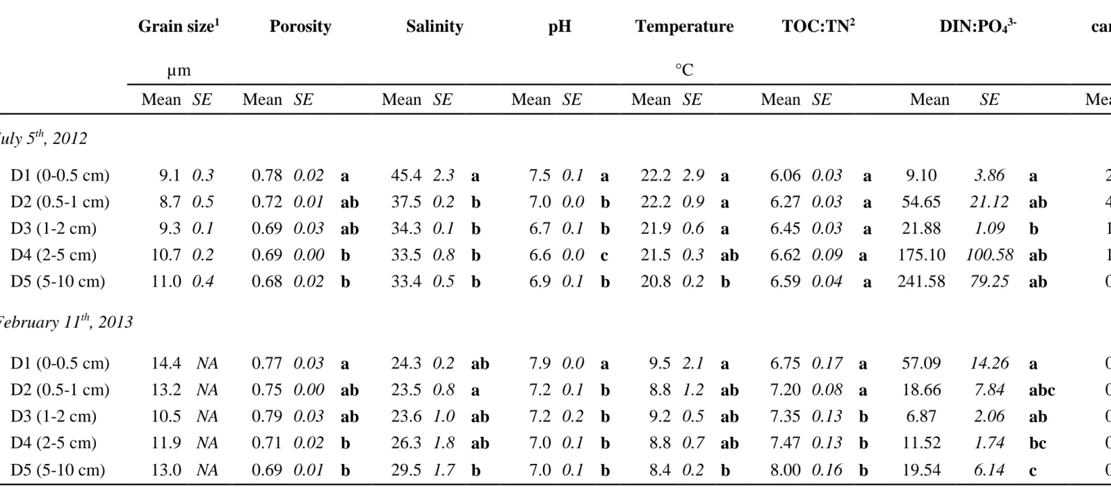
Table 1. Average of each environmental variables and algal biomass (± SE) along sediment depths. Two-way ANOVA reveals always significant differences between the two sampling dates for all variables (p < 0.05),
317
letters in bold font indicate Tukey’s post hoc test for each sampling date.
318
Grain size
1Porosity
Salinity
pH
Temperature
TOC:TN
2DIN:PO
4
3-
EPS-
carbohydrates/EPS-protein
3Colloidal EPS / bound
EPS
3Algal biomass
(Chl a)
µm
°C
µg g
-1sed DW
Mean SE
Mean SE
Mean SE
Mean SE
Mean SE
Mean SE
Mean
SE
Mean
SE
Mean
SE
Mean SE
July 5
th, 2012
D1 (0-0.5 cm)
9.1 0.3
0.78 0.02 a
45.4 2.3 a
7.5 0.1 a
22.2 2.9 a
6.06 0.03 a
9.10
3.86
a
2,69
0,67
a
1,09
0,26
ns
69.5 2.35
a
D2 (0.5-1 cm)
8.7 0.5
0.72 0.01 ab
37.5 0.2 b
7.0 0.0 b
22.2 0.9 a
6.27 0.03 a
54.65
21.12 ab
4,39
2,07
a
6,89
3,15
ns
16.2 0.68
b
D3 (1-2 cm)
9.3 0.1
0.69 0.03 ab
34.3 0.1 b
6.7 0.1 b
21.9 0.6 a
6.45 0.03 a
21.88
1.09
b
1,89
0,31
a
3,2
0,97
ns
6.2 0.50
c
D4 (2-5 cm)
10.7 0.2
0.69 0.00 b
33.5 0.8 b
6.6 0.0 c
21.5 0.3 ab
6.62 0.09 a
175.10 100.58 ab
1,32
0,33
a
1,94
0,44
ns
2.7 0.23
d
D5 (5-10 cm)
11.0 0.4
0.68 0.02 b
33.4 0.5 b
6.9 0.1 b
20.8 0.2 b
6.59 0.04 a
241.58
79.25 ab
0,99
0,18
a
2,78
0,12
ns
1.5 0.16
e
February 11
th, 2013
D1 (0-0.5 cm)
14.4 NA
0.77 0.03 a
24.3 0.2 ab
7.9 0.0 a
9.5 2.1 a
6.75 0.17 a
57.09
14.26 a
0,24
0,01
ab
2,9
0,33
ns
59.4 1.72
a
D2 (0.5-1 cm)
13.2 NA
0.75 0.00 ab
23.5 0.8 a
7.2 0.1 b
8.8 1.2 ab
7.20 0.08 a
18.66
7.84
abc
0,27
0,01
ab
3,16
0,2
ns
10.7 0.95
b
D3 (1-2 cm)
10.5 NA
0.79 0.03 ab
23.6 1.0 ab
7.2 0.2 b
9.2 0.5 ab
7.35 0.13 b
6.87
2.06
ab
0,35
0,03
b
2,34
0,11
ns
6.9 0.42
b
D4 (2-5 cm)
11.9 NA
0.71 0.02 b
26.3 1.8 ab
7.0 0.1 b
8.8 0.7 ab
7.47 0.13 b
11.52
1.74
bc
0,29
0,01
ab
2,67
0,33
ns
6.3 0.54
b
D5 (5-10 cm)
13.0 NA
0.69 0.01 b
29.5 1.7 b
7.0 0.1 b
8.4 0.2 b
8.00 0.16 b
19.54
6.14
c
0,19
0,03
ac
2,15
0,29
ns
2.9 0.18
c
1
Note that triplicates were not available for grain size for February sampling (NA: not available)
2
TOC:TN : ratio of total organic carbon (TOC) to total nitrogen (TN). TOC and TN are in µg g
-1sed DW
3
EPS-carbohydrates/EPS-protein and colloidal EPS/bound EPS are ratios without unit. Colloidal EPS-proteins, bound EPS-proteins, colloidal EPS-carbohydrates and bound EPS-carbohydrates are in µg g
-1sed DW.
16 320
Figure 1. Principal component analysis (PCA) ordination calculated using 8 physico-chemical
321
variables for a and c) 15 samples in July and b and d) 15 samples in February. a and b) 322
Ordination of the variables and correlation circle. b and d) Position of the observations in the 323
ordination; tree calculated hierarchical classification on principle components and the different 324
clusters evaluated using 10000 iterations . T: temperature; S: salinity; Prot: total protein 325
concentration; EPS.CB: colloidal EPS/bound EPS ratio; EPS.CP: EPS-carbohydrates/EPS-326
proteins ratio; DIN.P: DIN:PO43- ratio; TOC:TN: ratio of total organic carbon (TOC) and total 327
nitrogen (TN). PCA and hierarchical classification were performed using “FactoMineR” 328
package (Husson et al., 2013). 329
17
5.2 Prokaryotic abundances and activities
330
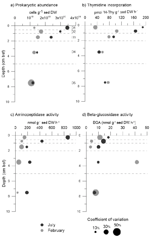
Prokaryotic abundances ranged from 1.18 ± 0.20 1010 to 3.45 ± 1.05 1010 cells g-1 sed DW 331
in July with maximum values in the surficial sediment layer (0-0.5 cm below the sediment 332
surface) (Figure 2). Abundances were significantly lower in February than in July (two-way 333
ANOVA, F=24.16, p < 0.001, Supp info Table S3) with values between 1.08 ± 0.75 1010 and 334
1.72 ± 0.50 1010 cells g-1 sed DW and a peak recorded between 0.5 and 1 cm bsf. In July, 335
thymidine incorporation (a proxy for benthic bacterial production) decreased with depth from 336
189.69 ± 8.15 to 46.31 ± 9.93 pmol 3H-Thy g-1 sed DW h-1. In February, thymidine 337
incorporation was lower but showed a similar decrease with depth. For both sampling dates, 338
thymidine incorporation and prokaryotic abundance distribution profiles were very similar 339
(Pearson test, n=30r2 = 0.806, p < 0.001) (Figure 2). The impact of a 10°C-increase on 340
thymidine production was expressed by using Q10. The temperature had a strong impact on 341
thymidine production between 0 and 0.5 cm bsf (average value of Q10=6.265). Then, between 342
0.5 and 1 cm bsf, temperature effect was less important (average value of Q10=1.589) but 343
significantly different from 1 (t-test one sample, t= 3.4589, p = 0,009). Between 1 and 10 cm 344
bsf, the temperature had no effect as Q10 values were not significantly different from 1 (t-test 345
one sample, p > 0.01). 346
Variance analysis (two-way ANOVA) showed that potential aminopeptidase activity was 347
significantly higher in July (F=75.29, p < 0.001, Supp info Table S3) (mean for all depth: 381.31 348
± 78.64 nmol g-1 sed DW h-1) than in February (mean for all depth: 88.02 ± 13.60 nmol g-1 sed 349
DW h-1) and that in July, these activities were significantly different in the surface sediment 350
compared to the deeper layers (Tukey HSD test, p < 0.001) (Figure 2). Potential β-glucosidase 351
activity was generally low throughout all the sediment depths. Values ranged from 6.71 ± 1.09 352
18
to 18.14 ± 1.42 nmol g-1 sed DW h-1 in July and from 3.49 ± 1.21 to 41.59 ± 8.32 nmol g-1 sed 353
DW h-1 in February (Figure 2). 354
19 355
Figure 2. Prokaryotic abundances, production and activities along a vertical depth
356
gradient below the sediment surface (bsf). All points represent the middle of each layer. The 357
coefficient of variation is displayed as bubble size. Black bubbles represent values for July 5, 358
2012, and gray bubbles represent values for February 11, 2013. 359
20
5.3 Algal biomass
360
The algal biomass on the surface (D1) was 69.5 ±2.4 µg Chl a g-1 sed DW 59.4 ±1.7 µg 361
Chl a g-1 sed DW during the samplings in July and in February, respectively (Table 1). The 362
highest standard errors were recorded in D1, resulting probably from the patchiness distribution 363
of the microphytobenthos observed in the field. The algal biomass showed an exponential 364
decrease with values never exceeding 17.40 µg Chl a g-1 sed DW under 0.5 cm bsf (Table 1). 365
5.4 The distribution of fauna abundances
366
The abundance of six meiofaunal groups was recorded: nematods, copepods, ostracods, small 367
gastropods, small bivalves and foraminifera (Supp info Fig S5). The most abundant were the 368
nematods (maximum abundance= 1060 ind cm-3) and foraminifera (maximum abundance= 57 369
ind cm-3). The abundances of groups investigated decreased with depth increase (Supp info Fig. 370
S5). Higher abundances were recorded in July except for copepods and ostracods. Additionally, 371
the macrozoobenthic grazer, Peringia ulvae (Pennant, 1777) present at the surface of the 372
sediment appeared to be more abundant in February (1908 ind m-2) than in July (528 ind m-2). 373
5.5 Factors influencing prokaryotic activities and densities
374
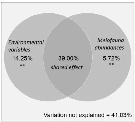
All variables used in the variation partitioning analysis (E table: salinity, phosphate and 375
silicate concentrations and M table: juvenile gastropods) had a significant effect on prokaryotic 376
activity and abundance (Supp info Table S4). The environmental variables (E table) explained 377
14.25 % of the variance of distribution of the prokaryote-related variables without the 378
component variations shared with the meiofauna abundance (M table). While meiofaunal 379
abundances explained 5.72% of the variation of prokaryotic variables. Collectively, phosphate 380
and silicate concentrations, salinity, and abundances of little gastropods explained 59% of the 381
prokaryotic abundances and activity variations (Figure 3). 382
21 383
Figure 3. Venn diagram based on a variation partitioning from prokaryotic variables
384
(i.e., prokaryotic abundance; thymidine incorporation; aminopeptidase activity; and beta-385
glucosidase activity). The external square represents the whole variation of the prokaryotic 386
table. Each circle represents the explanatory tables and values are the part of the variation 387
explained by each explanatory table. The variables used in the analysis was previously selected 388
by forward selection and final tables included: Environmental variable table: Salinity, PO4 3-389
concentrations, and silicate concentrations; and meiofauna table: abundances of juvenile 390
gastropods. Statistically significant pure fraction of variation of prokaryotes communities are 391
presented as: <0.01 ** (ANOVA like permutation test, 9999 permutations) and details are given 392
in Supp info Table S4. 393
22
6 Discussion
394
The muddy sediments in Marennes-Oléron Bay support high microbial activities and 395
production rates as is typical for fine-grained sediments (Böer, 2008; Llobet-Brossa et al., 396
1998). This study shows depth gradients of prokaryotic abundances and activities in the top 10-397
cm of these coastal mudflats based on the analyses of depth layers chosen to characterize 398
centimetre-scale processes. The stratification was particularly pronounced for the sampling in 399
July and this appeared to be related to depth variation of abiotic and biotic environmental 400
variables. Using the set of these environmental variables in the different depth layers, we have 401
studied how they could statistically explain the differences of prokaryotic abundances and 402
activities in the sediment. However, we had to exclude grain size and oxygen. The former 403
showed hardly any variation with depth, while the latter is known to show mm-scale variation 404
close to the surface that was not adequately measured in this study. Nevertheless, a sufficiently 405
large panel of biotic and abiotic variables were available for disentangling the contributions of 406
these environmental variables for driving prokaryotic abundances and activities. 407
6.1 Relative impact of environmental variables and meiofauna: the main driving factors
408
A forward selection identified that prokaryotic abundances and activities were 409
significantly influenced by salinity, phosphate and silicate concentrations as well as juvenile 410
gasteropod abundances. Above all, the resulting variation partition, underlined that the 411
interaction among physicochemical variables and meiofaunal abundance is high and has a 412
significant impact on prokaryotic abundances and activities (Figure 3). While the gasteropod 413
juveniles are not abundant in this study, their distribution significantly affects the prokaryotic-414
related variables and is strongly related to physicochemical variables (i.e., large part of variance 415
explanation shared with environmental table). 416
23
Nitrites or nitrates are more often identified as forcing factors for prokaryotic 417
communities in sediments (Böer et al., 2009), however, in the current study, the use of variation 418
partition shows that others inorganic nutrients such as silicates and phosphates significantly 419
influenced the prokaryotic activities and abundances. Interestingly, the phosphate 420
concentrations appeared to limit the prokaryotic activities (e.g., thymidine incorporation, 421
aminopeptidase and beta-glucosidase activities) more than nitrogen-related nutrients in bottom 422
layers in July and in surface in February (i.e. DIN:PO43- ratio>16; Supp info Figure S2). 423
In a previous study, Pascal et al. (2009) showed that only 6 % of the total bacterial 424
biomass was controlled by consumers in the first 1 cm of the sediment surface, suggesting a 425
major effect of resources in the Marennes-Oléron mudflat. Our statistical results suggest that 426
the activities and abundances of benthic prokaryotes in the first 10 cm of sediment were more 427
influenced by physicochemical properties of the sediment (i.e., inorganic nutrients and salinity) 428
rather than by predation pressure by meiofauna (Supp info Table S4). The variation partitioning 429
that we propose statistically identifies that bottom-up control (represented by physicochemical 430
variables) had stronger influence on prokaryotic activities than top-down control by meiofauna 431
and that the shared interactions between the two trophic controls are of major importance. In 432
the current study, it appears that physicochemical properties of the sediment that varied with 433
depth strongly stratified the biotic communities. The high part of variation explained by the two 434
trophic controls could reflects this influence of physicochemical variables on both prokaryotic 435
activities and abundances and meiofauna abundances. However, it could also be due to the fact 436
that meiofauna could slightly modifies the vertical stratification of organic matter, inorganic 437
nutrient or EPS composition. Other proxies can be used to identify factors that drive microbial 438
communities. For example, Pace & Cole (1994) proposed that a strong positive correlation 439
between prokaryotic biomass and production rates indicates bottom-up control. This relation 440
24
can thus be successfully applied to understand the relationships in benthic microbial ecology, 441
although other factors such as organic matter should also be considered. 442
6.2 Two horizons, two different stories
443
The principal component analysis followed by hierarchical clustering based on 444
physicochemical variables confirmed a vertical zonation mainly described by organic matter 445
composition (i.e., the TOC:TN ratio), pH and salinity (Figure 1). Collectively, our results 446
showed that the upper 10 cm of the sediment was divided into two clearly different horizons 447
with thickness varying between the samplings in July and February. The surface horizon, 448
separated from the bottom one by a transition layer is thicker in February (2 cm) than in July (1 449
cm). The position of the transition zone proposed here was therefore dependent on the thickness 450
of the sampling layers in our study and was expected to fluctuate from 1 cm to 3.5 cm bsf 451
(middle of our sampling layer). 452
The biotic and abiotic variables in the surface horizon differed between the two 453
sampling dates. In July, prokaryotic and environmental variables (e.g., prokaryotic abundance, 454
thymidine incorporation, aminopeptidase activity, EPS-carbohydrates and salinity) were high 455
compared to February (Table 1 and Figure 2). For example, in July, aminopeptidase activity 456
was particularly high compared to other studies (as reviewed by Danovaro et al. (2002)) but 457
comparable with aminopeptidase activities recorded in the Balearic Sea (Tholosan et al., 1999). 458
Thymidine incorporation, used as a proxy of benthic bacterial production, drastically increased 459
with an increase of 10°C (i.e., high Q10 value). On the basis of our results (Figure 2), we 460
hypothesized that in February, in the surface horizon (0-2 cm bsf), the prokaryotic communities 461
showing low metabolic activities were not able to sustain growth as a large part of their 462
metabolic energy was used for maintenance. In contrast, in July, as a result of higher 463
temperature, the high densities and high metabolic rates of prokaryotes seemed to be related to 464
metabolically active and growing populations. At low tide, prokaryotic populations in the 465
25
surface horizon are strongly influenced by external parameters (e.g., light exposure, 466
resuspension and tidal cycle) and microphytobenthic activity. Although algal biomass (i.e., as 467
measured by chlorophyll a concentration) was in the same range for both sampling dates, the 468
high microphytobenthic primary production in July (gross primary production: 6.0 ± 1.7 mg C 469
h-1 m-2, CO2 fluxes in benthic chambers measurement method, pers. comm. from J. Lavaud) 470
hadprobablyenhanced the bacterial production in the sediment top layer (0-0.5 cm bsf). This 471
source of labile carbon may be quickly transferred to the bacterial compartment as shown 472
previously in sandy sediments (Cook et al., 2007) and intertidal flats (Middelburg et al., 2000). 473
Moreover, large amounts of EPS-carbohydrates were recorded in July compared to February 474
and these EPS may be produced by epipelic diatoms in response to nutrient limitation or photo-475
protection (Smith and Underwood, 2000, 1998). Together, the high EPS-carbohydrates 476
concentrations, the low nutrient concentrations, and the DIN:PO43- ratio below the Redfield 477
value (Redfield, 1958), suggested a nitrogen limitation for benthic micro-organisms in surface 478
in July. 479
While EPS-carbohydrates were dominant in July, EPS-proteins clearly increased in 480
February (as shown by the shift of the ratio EPS-carbohydrates/EPS-proteins, Supp info Figure 481
S3). At this date, both prokaryotic density and thymidine incorporation were low in the top 482
horizon (0-2 cm bsf, Figure 2) and this was not only due to the low sediment temperature 483
because higher bacterial production occurred deeper in the sediment despite a similar 484
temperature. A study in Marennes-Oléron mudflat (Orvain et al., 2014b) shows that a higher 485
proportion of EPS-proteins coincided with mass erosion events and higher abundance of the 486
macrozoobenthic grazer, Peringia ulvae (Pennant, 1777). These macrozoobenthic grazers may 487
disturb the sediment stability by grazing on biofilm and EPS-proteins may potentially 488
originated from shell mucus (Orvain et al., 2014b). Based on these features and on our results, 489
it may be possible that the highest abundance of Peringia ulvae (Pennant, 1777) recorded in 490
26
February provoked a high predation pressure (i.e., predation pressure: 1.72 mg C h-1, calculated 491
according to Pascal et al. (2009)) and an increase of EPS-proteins, hence inducing mass erosion 492
of the sediment. This erosion is associated with the release of diatoms and prokaryotes into the 493
water column (Guizien et al., 2014; Montanié et al., 2014; Shimeta et al., 2002) and may 494
therefore impact the surface of sediment in February by a decrease of prokaryotic density and 495
bacterial production. Finally, in our study, even if mass erosion of the sediment surface might 496
have occurred at seeing the sea state (Suppl. Info, Table S2) and the wind speeds (data not 497
shown), prokaryotic abundance could be lower because of the grazing of Peringia ulvae 498
(Pennant, 1777) or by viral lysis that has been reported to be responsible for the loss of 40 % of 499
bacterial production in Marennes-Oléron mudflat (Saint-Béat et al., 2013). These results 500
suggesting a mass erosion event that occurred in February are consistent with a thicker surface 501
horizon (from 0 to 2 cm bsf) compared to the one in July. 502
In the bottom horizon, between 1 or 2cm bsf (in July and February, respectively) and 10 503
cm bsf, all biotic and physicochemical gradients showed little variation with depth. For both 504
sampling dates, the thymidine incorporation used as a proxy of bacterial production was similar 505
below 2 cm depth despite high environmental differences. Indeed, temperature, salinity, and 506
the EPS-carbohydrates strongly decreased from July to February, and nutrient concentrations 507
also changed—specifically, phosphate and ammonium concentrations increased (Supp info 508
Figure S2). While this bacterial production was clearly lower in this bottom horizon compared 509
to the surface one we probably underestimated thymidine uptake in the anoxic layers because 510
the experiments were not performed under anoxic conditions while microorganisms may be 511
partially or strictly anaerobes. Despite this potential underestimation, bacterial communities 512
were able to maintain the same production level between 2 and 10 cm bsf in both sampling 513
dates, suggesting that the system may potentially contain a low and stable microbial bulk 514
activity in this horizon throughout the year independently of environmental changes. 515
27
6.3 The transition zone
516
The boundary layer may represent a transition zone between the surface horizon largely 517
influenced by external parameters and the bottom horizon corresponding to reduced sediment. 518
The current study proposes that the transition zone should represent the limit of influence of 519
weather conditions on sediment physicochemical properties and thus on prokaryotic activities 520
in the intertidal mudflat. The depth of this layer was expected to fluctuate weakly over the 521
seasons and among the low tide period. Notably, storms can destroy the vertical structure deeper 522
than the external parameter-influenced zone. Nevertheless, except during these rare but strong 523
events, the depth of this surface layer can be considered specific to intertidal muddy sediments. 524
Indeed, sandy sediments are generally permeable and allow advective fluxes of water through 525
the interstitial spaces (Musat et al., 2006) and thus exhibit a different depth profile compared to 526
muddy sediments. Except for transient storms, the transition layer is thus located at 1-3.5 cm 527
depth in intertidal muddy sediments. 528
Whether this transition zone represents an environmental ecotone or ecocline can be 529
discussed. These two terms have been largely used in ecology to characterize boundary zones 530
where gradients occur, but their definitions and how to use them are still unclear (Erdôs et al., 531
2011). Nevertheless, many authors agree that the term environmental ecotone defines a gradient 532
between two adjacent habitats characterized by rather abrupt changes and that it comprises 533
habitats that should be very specific for certain species (Attrill and Rundle, 2002; Erdôs et al., 534
2011; van der Maarel, 1990; Whittaker, 1967). In contrast, an environmental ecocline stands 535
for more gradual changes that may result from mixing of the two communities from the 536
neighboring habitats (Attrill and Rundle, 2002; Erdôs et al., 2011; van der Maarel, 1990; 537
Whittaker, 1967). In the present study, the transition zone corresponded to a gradient zone at a 538
cm scale which we characterized by a gradual change of environmental variables such as 539
porosity or EPS ratios and a gradual change of microbial communities (e.g., algal biomass, 540
28
enzymatic activities and prokaryotic abundance). Hence, following these definitions and our 541
findings, we should rather consider the identified transition zone as an environmental ecoclinal 542
boundary (Erdôs et al., 2011). 543
6.4 Conclusion
544
The current study provided detailed snapshots of the depth gradients of prokaryotic 545
abundances and process rates at two sampling dates at low tide. The detailed stratification 546
pattern using a large ensemble of variables and different multivariate analyses allowed us to 547
decipher some of the major factors driving the densities and activities of microbial populations 548
in intertidal sediments. Thus, we succeeded in statistically explaining a large part of the 549
prokaryotic activity distributions by the environmental variables (i.e., salinity and nutrients), 550
and to a lesser extent by consumers (meiofauna), suggesting that bottom-up control was more 551
important than top-down control. In general we observed that the top 10 cm of these muddy 552
sediments comprise two clearly different depth horizons that are separated by a transition zone. 553
Thus we identified a surface horizon, which appears variable in thickness between sampling 554
dates and where prokaryotic activities and densities are highly impacted by microphytobenthic 555
activities and physicochemical variables and, a deeper and more stable bottom horizon. The 556
transition appears to be gradual corresponding to an environmental ecocline rather than an 557
ecotone. 558
Nevertheless, one part of this distribution remained statistically unexplained (41% of 559
the variation is estimated to be unresolved by the chosen variables in the variation partitioning) 560
and further studies are needed to explore 1) other abiotic variables such as sulfate, iron oxide 561
or manganese oxide concentration, 2) prokaryotic activity and production dynamics throughout 562
the low tide period, and 3) other prokaryotic indices such as diversity or functional genes. 563
29
7 Figure captions
564
Figure 1. Principal component analysis (PCA) ordination calculated using 8
physico-565
chemical variables for a and c) 15 samples in July and b and d) 15 samples in February. a and 566
b) Ordination of the variables and correlation circle. b and d) Position of the observations in the 567
ordination; tree calculated hierarchical classification on principle components and the different 568
clusters evaluated using 10000 iterations . T: temperature; S: salinity; Prot: total protein content; 569
EPS.CB: colloidal EPS/bound EPS ratio; EPS.CP: EPS-carbohydrates/EPS-protein ratio; 570
DIN.P: DIN:PO43- ratio; TOC:TN: ratio of total organic carbon (TOC) and total nitrogen (TN). 571
PCA and hierarchical classification were performed using “FactoMineR” package (Husson et 572
al., 2013). 573
Figure 2. Prokaryotic abundances, production and activities along a vertical depth
574
gradient below the sediment surface (bsf). All points represent the middle of each layer. The 575
coefficient of variation is displayed as bubble size. Black bubbles represent values for July 5, 576
2012, and gray bubbles represent values for February 11, 2013. 577
Figure 3. Venn diagram based on a variation partitioning from prokaryotic variables
578
(i.e., prokaryotic abundance; thymidine incorporation; aminopeptidase activity; and beta-579
glucosidase activity). The external square represents the whole variation of the prokaryotic 580
table. Each circle represents the explanatory tables and values are the part of the variation 581
explained by each explanatory table. The variables used in the analysis was previously selected 582
by forward selection and final tables included: Environmental variable table: Salinity, PO4 3-583
content, and silicate content; and meiofauna table: abundances of juvenile gastropods. 584
Statistically significant pure fraction of variation of prokaryotes communities are presented as: 585
<0.01 ** (ANOVA like permutation test, 9999 permutations) and details are given in Supp info 586
Table S4. 587
30
8 Table caption
588
Table 1. Average of each environmental variables and algal biomass (± SE) along 589
sediment depths. Two-way ANOVA reveals always significant differences between the two 590
sampling dates for all variables (p < 0.05), letters in bold font indicate Tukey’s post hoc test for 591
each sampling date. 592
31
9 Acknowledgments
594
This research was supported by a PhD grant (for Céline Lavergne) from the Charente 595
Maritime Department and by the French national program CPER 2006-2014 (Contrat Projet 596
Etat Région) of Charente Maritime, the French national program EC2CO (CAPABIOC, 2012-597
2014), and the CNRS (French National Center for Scientific Research). We acknowledge the 598
different analytical facilities in LIENSs laboratory: ‘Cytometry and imaging Facility’, 599
‘Radioactive Facility’, ‘Microbiological Facility’, and ‘Logistic, field Facility’. We are grateful 600
to K. Guizien and S. Lucas (LECOB, Banyuls s/ Mer, France), the LPO (French Bird Life 601
International organization) and D. Prevostat (Aeroglisseurs services) for their help in the field 602
and expertise. We also thank M. Le Goff (LEMAR, Plouzané, France) and PACHIDERM 603
analytical platform (Plouzané, France), V. Meleder (MMS, Nantes, France) and the analytic 604
platform of Geolittomer (UMR LETG, Nantes, France) for their expertise. Authors are grateful 605
to J. Lavaud and A. Barnett, I. Lanneluc, S. Sablé, I. Doghri, L. Beaugeard and J. Jourde. 606
Authors are also grateful to E. Desoche, A. Dupuy, C. Dussud and C. Le Kieffre. 607
32
10 References
608
Admiraal, W., 1984. The ecology of estuarine sediment inhabiting diatoms. Prog. Phycol. Res. 609
3, 269–314. 610
Agogué, H., Mallet, C., Orvain, F., De Crignis, M., Mornet, F., Dupuy, C., 2014. Bacterial 611
dynamics in a microphytobenthic biofilm: A tidal mesocosm approach. J. Sea Res. 92, 36– 612
45. doi:10.1016/j.seares.2014.03.003 613
Aminot, A., Kérouel, R., 2007. Dosage automatique des nutriments dans les eaux marines: 614
méthodes en flux continu. Ifremer. 615
Attrill, M.J., Rundle, S.D., 2002. Ecotone or Ecocline: Ecological Boundaries in Estuaries. 616
Estuar. Coast. Shelf Sci. 55, 929–936. doi:10.1006/ecss.2002.1036 617
Bertics, V.J., Ziebis, W., 2010. Bioturbation and the role of microniches for sulfate reduction 618
in coastal marine sediments. Environ. Microbiol. 12, 3022–3034. doi:10.1111/j.1462-619
2920.2010.02279.x 620
Bertics, V.J., Ziebis, W., 2009. Biodiversity of benthic microbial communities in bioturbated 621
coastal sediments is controlled by geochemical microniches. ISME J 3, 1269–1285. 622
Blott, S.J., Pye, K., 2001. GRADISTAT: a grain size distribution and statistics package for the 623
analysis of unconsolidated sediments. Earth Surf. Process. Landforms 26, 1237–1248. 624
doi:10.1002/esp.261 625
Böer, S., 2008. Investigation of the distribution and activity of benthic microorganisms in 626
coastal habitats. Bremen University. 627
Böer, S., Hedtkamp, S.I., van Beusekom, J.E., Fuhrman, J.A., Boetius, A., Ramette, A., 2009. 628
Time- and sediment depth-related variations in bacterial diversity and community 629
structure in subtidal sands. ISME J 3, 780–791. doi:10.1038/ismej.2009.29 630
Boetius, A., 1995. Microbial hydrolytic enzyme activities in deep-sea sediments. Helgoländer 631
Meeresuntersuchungen 49, 177–187. 632
Boetius, A., Lochte, K., 1996. Effect of organic enrichments on hydrolytic potentials and 633
growth of bacteria in deep-sea sediments. Mar. Ecol. Prog. Ser. 140, 239–250. 634
doi:10.3354/meps140239 635
Borcard, D., Legendre, P., Drapeau, P., 1992. Partialling out the Spatial Component of 636
Ecological Variation. Ecology 73, 1045–1055. doi:10.2307/1940179 637
Cook, P.L.M., Veuger, B., Böer, S., Middelburg, J.J., 2007. Effect of nutrient availability on 638
carbon and nitrogen incorporation and flows through benthic algae and bacteria in near-639
shore sandy sediment. Aquat. Microb. Ecol. 49, 165–180. doi:10.3354/ame01142 640
Danovaro, R., Manini, E., Fabiano, M., 2002. Exoenzymatic activity and organic matter 641
composition in sediments of the Northern Adriatic Sea: response to a river plume. Microb. 642
Ecol. 44, 235–251. doi:10.1007/s00248-002-1023-2 643
De Mesel, I., Derycke, S., Moens, T., Van der Gucht, K., Vincx, M., Swings, J., 2004. Top-644
down impact of bacterivorous nematodes on the bacterial community structure: a 645
microcosm study. Environ. Microbiol. 6, 733–744. doi:10.1111/j.1462-646
2920.2004.00610.x 647
Decho, A.W., 2000. Microbial biofilms in intertidal systems: an overview. Cont. Shelf Res. 20, 648