Ancient tropical extinctions at high latitudes contributed to the latitudinal diversity gradient*

HAL Id: hal-03049599

https://hal.archives-ouvertes.fr/hal-03049599

Submitted on 15 Dec 2020

HAL is a multi-disciplinary open access

archive for the deposit and dissemination of sci-entific research documents, whether they are pub-lished or not. The documents may come from teaching and research institutions in France or abroad, or from public or private research centers.

L’archive ouverte pluridisciplinaire HAL, est destinée au dépôt et à la diffusion de documents scientifiques de niveau recherche, publiés ou non, émanant des établissements d’enseignement et de recherche français ou étrangers, des laboratoires publics ou privés.

Ancient tropical extinctions at high latitudes

contributed to the latitudinal diversity gradient*

Andrea S. Meseguer, Fabien L. Condamine

To cite this version:

Andrea S. Meseguer, Fabien L. Condamine. Ancient tropical extinctions at high latitudes contributed to the latitudinal diversity gradient*. Evolution - International Journal of Organic Evolution, Wiley, 2020, 74 (9), pp.1966-1987. �10.1111/evo.13967�. �hal-03049599�

(i) Title: Ancient tropical extinctions at high latitudes contributed to the

1

latitudinal diversity gradient

2

(ii) Running title: Asymmetric gradient of tropical extinction

3

(iii) Authors: Andrea S. Meseguer

1,2,3

_{and Fabien L. Condamine}

2

4

(iv) Affiliations:

1

_{INRA, UMR 1062 Centre de Biologie pour la Gestion des}

5

Populations (INRA | IRD | CIRAD | Montpellier SupAgro), Montferrier-sur-Lez,

6

France.

2

_{CNRS, UMR 5554 Institut des Sciences de l’Evolution de Montpellier}

7

(Université de Montpellier | CNRS | IRD | EPHE), Montpellier, France.

3

_Real

8

Jardín Botánico de Madrid (RJB-CSIC), Madrid, Spain

9

(v) Corresponding author: Andrea S. Meseguer

10

(asanchezmeseguer@gmail.com)

11

(vi) Author contributions: A.S.M and F.L.C. designed the study, and analysed the

12

data; A.S.M wrote the paper with contributions of F.L.C.

13

(vii) Acknowledgments:

This preprint has been reviewed and recommended by

14

Peer Community In Evolutionary Biology (https://dx.doi.org/10.24072

15

/pci.evolbiol.100068). The authors are very grateful to Drs. T. Ezard, J. Hortal, J.

16

Arroyo, A. Mooers, J. Calatayud, and to the various anonymous reviewers for

17

comments and suggestions that greatly improved the study. Previous versions of

18

the manuscript benefited from the comments of Drs. G. Mittlebach, E. Jousselin

19

and J. Rolland. Financial support was provided by a Marie-Curie FP7–COFUND

20

(AgreenSkills fellowship–26719) grant to A.S.M. and a Marie Curie FP7-IOF

21

(project 627684 BIOMME) grant to F.L.C. This work benefited from an

22

“Investissements d’Avenir” grant managed by the “Agence Nationale de la

23

Recherche” (CEBA, ref. ANR-10-LABX-25-01).

24

(viii) Data Accessibility Statement:

25

The datasets supporting the results, the commands used in the analyses and the

26

Appendix 1 are stored in

Dryad, https://doi.org/10.5061/dryad.zs7h44j5m.

27

Abstract

28

Global biodiversity currently peaks at the equator and decreases toward the poles.

29

Growing fossil evidence suggest this hump-shaped latitudinal diversity gradient (LDG)

30

has not been persistent through time, with similar diversity across latitudes flattening

31

out the LDG during past greenhouse periods. However, when and how diversity declined

32

at high latitudes to generate the modern LDG remains an open question. Although

33

diversity-loss scenarios have been proposed, they remain mostly undemonstrated. We

34

outline the ‘asymmetric gradient of extinction and dispersal’ framework that

35

contextualizes previous ideas behind the LDG under a time-variable scenario. Using

36

phylogenies and fossils of Testudines, Crocodilia and Lepidosauria, we find that the

37

hump-shaped LDG could be explained by (1) disproportionate extinctions of

high-38

latitude tropical-adapted clades when climate transitioned from greenhouse to

39

icehouse, and (2) equator-ward biotic dispersals tracking their climatic preferences

40

when tropical biomes became restricted to the equator. Conversely, equivalent

41

diversification rates across latitudes can account for the formation of an ancient flat

42

LDG. The inclusion of fossils in macroevolutionary studies allows revealing

time-43

dependent extinction rates hardly detectable from phylogenies only. This study

44

underscores that the prevailing evolutionary processes generating the LDG during

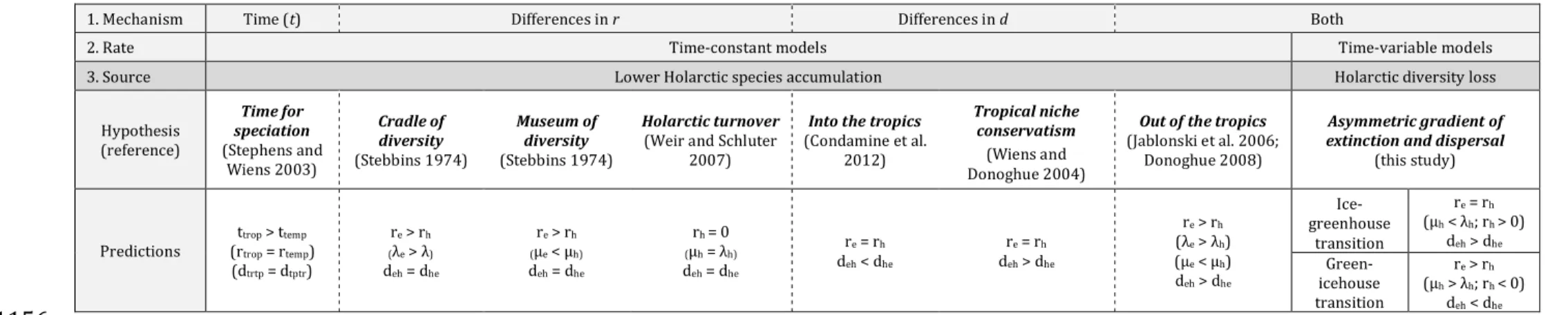
45

greenhouses differed from those operating during icehouses.

46

47

Keywords: biodiversity; climate change; extinction; fossils; Holarctic; tropics

48

49

Introduction

50

The current increase in species richness from the poles toward the equator, known as

51

the latitudinal diversity gradient (LDG), is one of the most conspicuous patterns in

52

ecology and evolution. This pattern has been described for microbes, insects,

53

vertebrates, and plants, and for marine, freshwater, and terrestrial ecosystems (Willig et

54

al. 2003; Hillebrand 2004; Novotny et al. 2006; Kreft and Jetz 2007; Fuhrman et al.

55

2008; Jenkins et al. 2013).

56

For decades, it has been thought that the modern steep LDG, with higher

57

diversity concentrated at the equator, persisted throughout the Phanerozoic (the last

58

540 million years), even if the gradient was sometimes shallower (Mittelbach et al.

59

2007), based on published fossil record studies (Crame 2001; Alroy et al. 2008).

60

However, the methodological limitations of fossil sampling have called this conclusion

61

into question. Analyses controlling for sampling bias have suggested that, for many

62

groups, the LDG was less marked in the past than it is today (i.e. with similar species

63

diversity across latitudes) or even developed a paleotemperate peak during some

64

periods (see Mannion et al. (2014) for a review). This sampling-corrected flattened LDG

65

in deep time has been demonstrated for non-avian dinosaurs (Mannion et al. 2012),

66

mammals (Rose et al. 2011; Marcot et al. 2016), birds (Saupe et al. 2019a), tetrapods

67

(Brocklehurst et al. 2017), insects (Archibald et al. 2010, 2013; Labandeira and Currano

68

2013), brachiopods (Krug and Patzkowsky 2007; Powell 2007; Powell et al. 2012),

69

bivalves (Crame 2000, 2020), coral reefs (Leprieur et al. 2016), foraminifers (Fenton et

70

al. 2016), crocodiles (Mannion et al. 2015), turtles (Nicholson et al. 2015, 2016), or

71

plants (Coiffard and Gomez 2012; Peralta-Medina and Falcon-Lang 2012; Shiono et al.

72

2018).

73

The pattern emerging from fossil studies also suggests that steep LDGs, such as

74

that currently observed, have been restricted to the relatively small number of short

icehouse periods during the Earth’s history: the Ordovician/Silurian, the

76

Carboniferous/Permian, and the Neogene. Most of the Phanerozoic has instead been

77

characterized by warm greenhouse climates associated with a flatter LDG (Mannion et

78

al. 2014; Marcot et al. 2016). Hence, the last change in the shape of the LDG

79

hypothetically occurred during the greenhouse to icehouse transition of the Cenozoic, in

80

the last 66 million years (Fig. 1).

81

82

Figure 1. Changes in global temperatures and extension of the tropical belt during the Cenozoic, in relation

83

with the shape of the LDG. Early Cenozoic global temperatures were higher than today and paratropical

84

conditions extended over high latitudes. From the early Eocene climatic optimum (EECO; ca. 53-51 Ma), a

85

global cooling trend intensified and culminated with the Pleistocene glaciations. Warm-equable regimes got

86

then restricted to the equator. The LDG evolved following these global changes; during greenhouse periods

87

diversity was similar across latitudes, such that the LDG flattened, while in cold periods diversity peaked at

88

the equator (a steep LDG) (Mannion et al. 2014). The question mark denotes the focus of this study, which is

89

to unveil the processes that mediated the transition between a flat and steep LDG. The relative temperature

90

curve of the Cenozoic is adapted from (Zachos et al. 2008). Maps represent the extension of the tropical belt

91

and Earth tectonic changes as derived from (Ziegler et al. 2003; Morley 2007). P=Pleistocene, Pli=Pliocene.

92

93

94

95

Our perception on how diversity was latitudinally distributed in the past

96

underlies LDG interpretations. Up to now, most studies have assumed the equator is the

97

source of world diversity (Donoghue 2008; Jablonski et al. 2013) and diversity was

98

always lower in the Holarctic (i.e. a steep LDG persisted in the deep time). The current

99

shape of the LDG thus results from lower paces of diversity accumulation in the

100

Holarctic than at the equator through time. Slower diversity accumulation in the

101

Holarctic (hereafter ‘H’) have been explained either by greater tropical diversification

102

and limited dispersal out of the equatorial region (hereafter ‘equator’ or ‘E’) (re > rh ; deh

103

> dhe) (Latham and Ricklefs 1993; Wiens and Donoghue 2004; Mittelbach et al. 2007;

104

Rolland et al. 2014), or by high rates of turnover in the Holarctic, i.e. similar high

105

speciation (λ) and extinction (μ) rates (!h ≈ µh; Table 1). This has been widely shown

106

throughout the tree of life: amphibians (Wiens 2007; Pyron and Wiens 2013), birds

(Cardillo et al. 2005; Ricklefs 2006; Weir and Schluter 2007), butterflies (Condamine et

108

al. 2012), plants (Leslie et al. 2012; Kerkhoff et al. 2014), fishes (Siqueira et al. 2016),

109

mammals (Weir and Schluter 2007; Rolland et al. 2014), or lepidosaurs (Pyron 2014).

110

Contrary to the ‘slow Holarctic diversity accumulation’ hypotheses, a scenario

111

assuming the Holarctic was also a source of tropical diversity that flattened the LDG in

112

the deep past could be considered. The current steep shape of the LDG would thus result

113

from diversity lost in the Holarctic through evolutionary time, referred to as the

114

´Holarctic diversity loss’ hypothesis. The recent fossil investigations showing, for many

115

lineages, similar diversity levels across latitudes in the past lend support to this

116

scenario, suggesting we do not necessarily need to explain why diversity accumulated at

117

slower rates in the Holarctic through time, but the question being how and when

118

diversity was lost at high latitudes, giving rise to the current shape of the LDG (Mannion

119

et al. 2014)?

120

Diversity losses in the Holarctic have been traditionally considered to underlie

121

the LDG. They were initially attributed to Pleistocene glaciations (Martin and Klein

122

1989), but this hypothesis can be called into question since the LDG substantially

123

predates the Pleistocene (Mittelbach et al. 2007). More ancient extinctions have also

124

been considered (Latham and Ricklefs 1993; Markwick 1998; Roy and Pandolfi 2005;

125

Hawkins et al. 2006; Weir and Schluter 2007; Dunn et al. 2009; Eiserhardt et al. 2015;

126

Pulido-Santacruz and Weir 2016). For example, recent studies suggested the avian LDG

127

resulted from the differential extirpation of older warm-adapted clades from the

128

temperate regions newly formed in the Neogene (Hawkins et al. 2006; Pulido-Santacruz

129

and Weir 2016; Saupe et al. 2019a). Pyron (2014) suggested that higher temperate

130

extinction represents a dominant force for the origin of LDG in lepidosaurs. Wiens &

131

Donoghue (2004) also proposed that range contractions (deh < dhe) followed climate

132

cooling.

Unfortunately, using phylogenies of extant taxa alone, studies on the LDG have

134

not clearly demonstrated diversity losses in the Holarctic but instead high regional

135

turnover (! ≈ µ) (Cardillo et al. 2005; Weir and Schluter 2007; Condamine et al. 2012;

136

Leslie et al. 2012; Pyron and Wiens 2013; Rolland et al. 2014, 2015; Rabosky et al.

137

2018). Nonetheless, high turnover in the Holarctic can only explain a slow accumulation

138

of lineages, with one fauna being replaced by another, but does not explain diversity

139

decline (i.e. a reduction in the net number of species) as elevated speciation rates

140

counter-balance the effect of extinction. Diversity declines occur when extinction

141

exceeds speciation ($ > !), resulting in negative net diversification rates (% = ! − µ; % < 0).

142

Accordingly, ‘diversity loss’ hypotheses differ from ‘high turnover’ scenarios.

143

The perceived difficulty for inferring negative diversification rates from

144

phylogenetic data of extant species (Rabosky 2010; Burin et al. 2018) and the

145

assumption that diversity levels always remained lower in the Holarctic than at the

146

equator have resulted in ‘diversity loss’ hypotheses being repeatedly proposed but

147

seldom demonstrated using phylogenetic data (Pulido-Santacruz and Weir 2016).

148

Meanwhile, numerous fossil investigations have detected signatures of extinction and

149

diversity loss in the Northern Hemisphere. For instance, Archibald et al. (2010, 2013)

150

sampled insect diversity at an Eocene site in Canada, and in present-day temperate

151

Massachusetts (USA) and tropical sites of Costa Rica. Insect diversity was higher at the

152

Eocene paleotropical site than the modern temperate locality, and comparable to the

153

modern-day tropical locality, suggesting that post-Eocene Nearctic insects have suffered

154

great levels of extinction. This pattern is consistent with other studies on various

155

taxonomic groups, including birds (Mayr 2016), invertebrates (Wilf et al. 2005),

156

mammals (Blois and Hadly 2009; Rose et al. 2011; Marcot et al. 2016), and plants

157

(Frederiksen 1988; Smith and al. 2012; Xing et al. 2014). Fossil studies are, however,

158

generally restricted to a reduced geographic and temporal scale, which makes difficult

159

to extrapolate local inferences of extinction in the global context of the LDG.

Here, we use comparative methods for both phylogenies and fossils to estimate

161

the evolutionary processes behind the LDG of Testudines, Crocodilia and Lepidosauria,

162

and test the alternative predictions of two hypotheses: “slow diversity accumulation”

163

(deh > dhe; $h ≤ !h) vs. “diversity loss” (deh < dhe; $h > !h) in the Holarctic. To this end, we

164

propose to include a temporal component to study the LDG in which prevailing

165

speciation, extinction and dispersal dynamics may change between warm- and cold-time

166

intervals. The extant Crocodilia and Lepidosauria comprise mostly tropical-adapted

167

species with a classic LDG pattern as shown by diversity peaks at equatorial latitudes

168

(Markwick 1998; Pyron 2014). We investigate the origin of the LDG in subtropical taxa

169

as well, by extending the study to Testudines, which display a hump-shaped gradient of

170

diversity centered on subtropical latitudes (10°S–30ºN) (Angielczyk et al. 2015). By

171

contrast, the paleolatitudinal distribution of turtles was concentrated in the Holarctic

172

(30–60ºN) during the Cretaceous (Nicholson et al. 2015, 2016). All these lineages are

173

ancient and likely experienced climatic transitions during the early Cenozoic (Markwick

174

1998; Pyron 2014; Angielczyk et al. 2015; Mannion et al. 2015; Nicholson et al. 2015).

175

They show contrasting patterns of species richness: turtles and crocodiles are species-176

poor (350 and 25 species, respectively), while lepidosaurs include a large number of

177

species (10,000+ species), and all have a rich fossil record extending back to the Triassic

178

(Early Cretaceous for crocodiles), providing information about the variation of

179

latitudinal species richness accumulation during their evolutionary history.

180

Methods

181

Molecular phylogenies and the fossil record. A time-calibrated phylogeny for turtles

182

(order Testudines) was obtained from Jaffe et al. _{(2011), including 233 species. We}

183

preferred this phylogeny over other more recent and slightly better sampled trees

184

(Rodrigues and Diniz-Filho 2016) because the divergence time estimates are more

consistent with recent estimates based on genomic datasets (Pereira et al. 2017; Shaffer

186

et al. 2017). For scaled lizards (Lepidosauria), we retrieved the most comprehensive

187

dated tree available, including 4161 species (Pyron 2014), and a complete phylogeny

188

was obtained for crocodiles (Crocodilia) (Oaks 2011).

189

Fossil occurrences were downloaded from the Paleobiology Database

190

(https://paleobiodb.org/#/, last accessed October 25th _{2017). We reduced potential}

191

biases in the taxonomic assignation of turtle, crocodile and lepidosaur fossils, by

192

compiling occurrence data at the genus level. We further cleaned the fossil datasets by

193

checking for synonymies between taxa and for assignment to a particular genus or

194

family on the basis of published results.

195

196

Estimation of origination and extinction rates with phylogenies. We ensured

197

comparability with previous LDG studies and investigated possible differences between

198

Holarctic and equatorial regions by combining the turtle and lepidosaur phylogenies

199

with distributional data to fit trait-dependent diversification models in BiSSE (Maddison

200

et al. 2007). We accounted for incomplete taxon sampling in the form of trait-specific

201

global sampling fraction (FitzJohn et al. 2009). We did not use the geographic-state

202

speciation and extinction model (Goldberg et al. 2011), which is appropriate for dealing

203

with widespread species, because most of the species in our datasets were endemic to

204

the Holarctic or equatorial regions (see below), and, for a character state to be

205

considered in SSE models, it must account for at least 10% of the total diversity (Davis et

206

al. 2013). We did not apply the BiSSE model to crocodiles, because simulations have

207

shown that trees containing fewer than 300 species may have too weak a phylogenetic

208

signal to generate sufficient statistical power (Davis et al. 2013).

209

We initially implemented a constant-rate BiSSE model in the R-package

210

diversitree 0.9-7 (FitzJohn 2012) with six parameters: two speciation rates, one

211

associated with the Holarctic (‘H’, λH) and the other with other equatorial and

subtropical regions (‘equator’ or ‘E’, λE), two extinction rates associated with the

213

Holarctic (μH) and the equator (μE), and two transition rates (dispersal), one for the

214

Holarctic to equator direction (qHE), and the other for the equator to Holarctic direction

215

(qEH). We categorized each species as living in the equator or the Holarctic according to

216

the threshold latitudes defining the tropics (23.4°N and 23.4°S). According to our

217

distribution data, 84% of extant species of turtles, lepidosaurs and crocodiles lives in the

218

tropics, 15% in temperate regions and 1% span both biomes. For turtles, there were 239

219

tropical species, 84 temperate and 6 spanning both biomes (7 were marine). For

220

lepidosaurs, 7955 tropical, 1337 temperate and 124 spanning both biomes. Crocodiles

221

had 23 tropical and two temperate species (Tables S1-3).

222

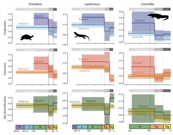
We then used the time-dependent BiSSE (BiSSE.td) model, in which speciation,

223

extinction, and dispersal rates are allowed to vary between regions and to change after

224

shift times. We introduced two shift times to model different diversification dynamics

225

between greenhouse, transitional, and icehouse periods. We assumed that a global

226

warm tropical-like climate dominated the world from the origin of the clades until 51

227

Ma (corresponding to the temperature peak of the Cenozoic). Thereafter, the climate

228

progressively cooled until 23 Ma (the transitional period), when the climate definitively

229

shifted to a temperate-like biome in the Holarctic (Ziegler et al. 2003; Morley 2007;

230

Zachos et al. 2008). The climatic transition in the Cenozoic may have different temporal

231

boundaries, with potential effects on the results. We thus applied the same model but

232

with different combinations of shift times (we tested 51/66 Ma and 23/34 Ma for the

233

upper and lower bounds of the climatic transition). We used a Markov Chain Monte

234

Carlo (MCMC) approach to investigate the credibility intervals of the parameter

235

estimates, with an exponential prior 1/(2r) and initiated the chain with the parameters

236

obtained by maximum likelihood. We ran 10,000 MCMC steps, with a burn-in of 10%.

237

238

Estimation of origination and extinction rates with fossils. We analyzed the three

239

fossil records using a Bayesian model implemented in PyRate (Silvestro et al. 2019) for

240

simultaneous inference of the temporal dynamics of origination and extinction, and of

241

preservation rates (Silvestro et al. 2014). The turtle fossil dataset contains 4084

242

occurrences for 420 genera (65 extant and 355 extinct; Table S4). The lepidosaur fossil

243

dataset comprises 4798 occurrences for 638 genera (120 extant and 518 extinct; Table

244

S5). The crocodile fossil dataset includes 1596 occurrences for 121 genera (9 extant and

245

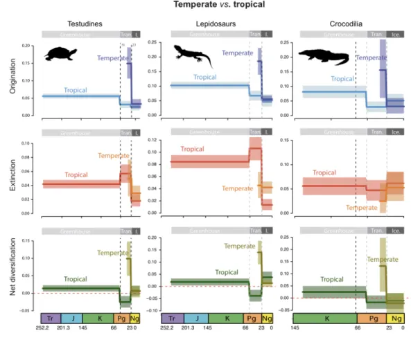
112 extinct; Table S6). In this analysis, the preservation process is used to infer the

246

individual origination and extinction times of each taxon from all fossil occurrences and

247

an estimated preservation rate expressed as expected occurrences per taxon per million

248

years. We followed a birth-death shift approach (Silvestro et al. 2015), also known as the

249

Bayesian skyline model, and used a homogeneous Poisson process of preservation

(-250

mHPP option). We used default settings and accounted for the variation of preservation

251

rates across taxa, using a Gamma model with gamma-distributed rate heterogeneity (-252

mG option) and four rate categories to discretize the gamma distribution.

253

Given the large number of occurrences analyzed and the vast timescale

254

considered, we dissected the birth–death process into time intervals, and estimated

255

origination and extinction rates within these intervals. In one set of analyses, we defined

256

time intervals using the geological epochs of the stratigraphic timescale (Ogg et al.

257

2004). In another set of analyses, we defined time intervals according to the major

258

climatic periods characterizing the Cenozoic: the greenhouse world, the climatic

259

transition, and the icehouse world, testing two alternatively boundaries for the climatic

260

transition in the Cenozoic (34/23 Ma). We adopted this solution as an alternative to the

261

algorithms implemented in the original PyRate software for joint estimation of the

262

number of rate shifts and the times at which origination and extinction shift (Silvestro et

263

al. 2014). The estimation of origination and extinction rates within fixed time intervals

264

improved the mixing of the MCMC and made it possible to obtain an overview of the

general trends in rate variation over a long timescale. Both the preservation and birth–

266

death processes were modelled in continuous time but without being based on

267

boundary crossings. One potential problem when fixing the number of rate shifts a

268

priori is over-parameterization. The Bayesian skyline model overcame this problem by

269

assuming that the rates of origination and extinction belonged to two families of

270

parameters following a common prior distribution, with parameters estimated from the

271

data with hyper-priors (Gelman 2004).

272

We ran PyRate for 10 million MCMC generations on each of the 10 randomly

273

replicated datasets. We monitored chain mixing and effective sample sizes by examining

274

the log files in Tracer 1.7 (Rambaut et al. 2018). After excluding the first 20% of the

275

samples as a burn-in, we combined the posterior estimates of the origination and

276

extinction rates across all replicates to generate plots of the change in rate over time.

277

The rates of two adjacent intervals were considered significantly different if the mean of

278

one lay outside the 95% credibility interval of the other, and vice versa.

279

In the context of the LDG, we performed additional analyses with different

280

subsets of fossils, to separate the speciation, extinction and preservation signals of

281

different geographic regions (equator or Holarctic) and ecological conditions

282

(temperate or tropical). For example, for turtles, we split the global fossil dataset into

283

four subsets: one for the fossil genera occurring at the equator (429 occurrences), one

284

for the fossils occurring in the Holarctic (3568 occurrences), one for the fossil genera

285

considered to be adapted to temperate conditions (993 occurrences), and one for the

286

fossils considered to be adapted to tropical conditions (2996 occurrences). We excluded

287

the few fossil occurrences for the southern regions of the South Hemisphere (about 180)

288

only in subset analyses, as they were poorly represented in our dataset. Note that a

289

given fossil can be present in both the ‘Holarctic’ and ‘tropical’ datasets. We encoded

290

tropical/temperate preferences by considering macro-conditions in the Holarctic to be

291

paratropical until the end of the Eocene, as previously reported (Ziegler et al. 2003;

Morley 2007). We also assumed that taxa inhabiting the warm Holarctic were adapted

293

to tropical-like conditions (i.e. a high global temperature, indicating probable adaptation

294

to tropical climates). After the late Eocene, we categorized each species as living in the

295

temperate biome as defined above. With these datasets, we reproduced the same PyRate

296

analyses as for the whole dataset.

297

Finally, we examined the apparent incongruence between paleontological and

298

phylogenetic estimates of diversification (see Results) using the birth-death

299

chronospecies (BDC) model in PyRate (Silvestro et al. 2018). This model allows

300

examining whether alternative speciation modes described for the fossil record, i.e.

301

budding, bifurcation or anagenesis (Silvestro et al. 2018), are responsible for driving

302

incongruences between fossil and phylogenetic estimates. We compared an (i) Equal

303

rates model where diversification parameters estimated with stratigraphic data (λ* and

304

μ*) are the same to those estimated with phylogenetic data (λ and μ), i.e. λ* = λ, μ* = μ;

305

(ii) a Compatible model where parameters differ, but the differences could be explained

306

by differences in speciation mode. In this model λ*, λ, μ, μ* are constrained such that λ* −

307

λ = μ* − μ (i.e. equal net diversification rates) and λ* ≥ λ; (iii) an Incompatible model,

308

where parameters λ, λ*, μ, μ* are allowed to take any value and thus differences in λ and

309

λ*, as well as μ and μ*, cannot be explained by differences in speciation mode.

310

We estimated λ, μ, λ*, μ* simultaneously for the Testudines, Crocodilia and

311

Lepidosauria phylogenies pruned to the genus level, and the corresponding fossil data

312

using maximum-likelihood optimization and assuming constant diversification rates

313

through time. To assess support for the BDC model we applied a likelihood ratio test

314

(Silvestro et al. 2018), comparing which of the equal, compatible or incompatible rates

315

models are supported by our data.

316

Since the evolutionary histories of Testudines, Lepidosauria and Crocodilia is

317

long and exhibit great amount of temporal heterogeneity in both speciation and

318

extinction rates (see results), we also implemented a Bayesian skyline model with rate

shifts at the climatic epoch boundaries defined above. We ran 10 million MCMC

320

iterations to obtain joint posterior distributions of the stratigraphic and phylogenetic

321

rates. We used the joint posterior samples of λ*, μ*, λ, and μ obtained under the

322

incompatible rates model to verify the conditions predicted by the compatible BDC

323

model (i.e. λ* − λ = μ* − μ and λ* ≥ λ) and assess the support for each model as suggested

324

in previous studies (Silvestro et al. 2018).

325

326

Inferring ancestral geographic distribution with phylogenies and fossils. We

327

performed biogeographic analyses with the parametric likelihood method DEC (Ree and

328

Smith 2008) using the fast C++ version (Smith 2009)

(https://github.com/rhr/lagrange-329

cpp). Turtle, lepidosaur, and crocodile species distributions were obtained from online

330

databases (www.iucnredlist.org and www.reptile-database.org). We also chose 23.4°N

331

and 23.4°S as the threshold latitudes defining the tropics, and categorized each species

332

as living in the Holarctic, in the southern temperate regions, or in the equatorial tropics

333

and subtropical regions. We considered that all ranges comprising three areas could be

334

considered an ancestral state (maxareas =3).

335

We set up three different DEC analyses. We first ran DEC with no particular

336

constraints, using only the distribution of extant species. We then performed DEC

337

analyses including fossil information in the form of ‘fossil constraints’ at certain nodes,

338

according to the range of distribution of fossil occurrences assigned to a particular taxon

339

during the relevant time frame. For example, the crown age of Carettochelyidae

340

(Testudines) dates back to the Late Jurassic (150 Ma), and we set a geographic

341

constraint on this node reflecting the distribution of all the Late Jurassic fossils

342

attributed to Carettochelyidae. Similarly, for the origin of turtles (210 Ma), distribution

343

constraints represent the range of Late Triassic fossils assigned to turtles.

344

We followed two different approaches to include fossil distributions. First, we

345

used a soft fossil constraints (SFC) approach to incorporate fossil data into the

anagenetic component of the likelihood framework. The direct impact of a given fossil is

347

limited to the particular branch to which it has been assigned, although it may indirectly

348

influence other branches. The inclusion of a fossil conditions the estimated geographic-349

transition probability matrix for that branch by imposing a spatiotemporal constraint on

350

the simulation process. Only the simulations resulting in a geographic range including

351

the area of fossil occurrence contribute to the geographic-range transition probability

352

matrix for the branch concerned; simulations not meeting this constraint are discarded

353

(Moore et al. 2008). This was achieved with existing functions in the C++ version of

354

Lagrange, using the command ‘fossil’. We consider this to be a ‘soft’ constraint, because

355

other areas different from that in which the fossil was found could be included in the

356

ancestral states. In some cases, the SFC model may still overlook known fossil

357

information. Second, we then implemented a hard fossil constraints (HFC) approach,

358

where the estimation of ancestral areas was fixed to the location of fossils. For HFC, we

359

used the command ‘fixnode’. By fixing nodes to the distribution area of fossils, we

360

assume fossil occurrences reflect the distribution of the ancestors. This is a strong

361

assumption, but it makes it possible to recover all fossil ranges in the ancestral

362

estimations. The real scenario probably lies somewhere between SFC and HFC

363

inferences.

364

We then compared the timing and number of range extinction and dispersal

365

events inferred with the three different biogeographic approaches through time. In DEC,

366

extinction (range contraction) and dispersal (range expansion) events are modeled as

367

stochastic processes occurring along the branches of the tree (Ree and Sanmartin 2009),

368

with the probability of any extinction/dispersal event to occur being constant along the

369

entire length of the branch. We therefore estimated the periods at which range

370

extinction and dispersal occurred by dividing the phylogeny into intervals of 25 million

371

years and calculating the number of branches for which extinction/dispersal was

inferred crossing a particular time interval (the same branch could cross two continuous

373

intervals).

374

Results

375

Phylogeny-based diversification analyses: are diversification rates higher at the

376

equator? Under the time-constant BiSSE model, net diversification rates for turtles were

377

higher in the Holarctic than at the equator (Fig. S1a), but this difference was not

378

significant, and rates of dispersal ‘into the equator’ were ten times higher than those ‘out

379

of the equator’. For lepidosaurs, a similar dispersal pattern was recovered, but net

380

diversification rates were significantly higher in the equator (Fig. S1b). The

time-381

variable BiSSE models, with shift times at 51 and 23 Ma, indicated that speciation and

382

extinction rates of turtles were similar in the Holarctic and at the equator until the

383

icehouse period, when Holarctic speciation increased. For lepidosaurs, speciation was

384

lower in the Holarctic and extinction higher until the icehouse period, when Holarctic

385

speciation increased and extinction decreased (Fig. S2). Dispersal was symmetric

386

between regions (into the equator = out of the equator) during greenhouse periods, and

387

asymmetric (into the equator > out of the equator) during the climatic transition and

388

icehouse period. The same patterns were obtained assuming different combinations of

389

shift times (51/66 Ma and 23/34 Ma; Fig. S3, S4).

390

391

Fossil-based diversification analyses: evidence for ancient tropical extinctions? We

392

first inferred global diversification dynamics by analyzing the fossil datasets as a whole.

393

For turtles, origination rates peaked during the Jurassic, subsequently decreasing until

394

the present. Extinction rates were generally low and constant during the Mesozoic, but

395

increased during the Jurassic and the Paleogene, resulting in negative net diversification

396

during the Paleogene only (Fig. 2). For lepidosaurs, origination rates peaked in the

Jurassic and Late Cretaceous, whereas extinction increased steadily until the Late

398

Cretaceous. In the Paleogene, net diversification approached zero, suggesting a high

399

turnover. Crocodile origination peaked in the Early Cretaceous, subsequently decreasing

400

toward the present, and extinction rates were generally low and constant. We also

401

identified diversity losses in the Paleogene extending to the present, suggesting that

402

crocodiles are still in a phase of declining diversity (Fig. 2).

403

404

Figure 2. Global pattern of turtle, lepidosaur, and crocodile diversification through time based on the fossil

405

record. Origination (blue) and extinction (red) rates were estimated using time bins as defined by epochs of

406

the geological timescale (on the top, main climatic periods are shown as follows: Greenhouse, Tran. =

407

climatic transition, and I. = icehouse). Solid lines indicate mean posterior rates, whereas the shaded areas

408

show 95% credibility intervals. Net diversification rates (green) are the difference between origination and

409

extinction. The vertical lines indicate the boundaries between geological periods. Tr=Triassic; J=Jurassic;

410

K=Cretaceous; Pg=Paleogene, and Ng=Neogene.

411

412

Additional analyses with different subsets of the three fossil datasets separating

413

origination and extinction signals between geographic regions (equator or Holarctic)

414

and ecological conditions (temperate or tropical), showed that the diversity losses

415

experienced by turtles and crocodiles during the Paleogene were mostly attributable to

416

species living in the Holarctic and under tropical conditions (Figs. 3, 4). The global

diversity loss inferred for crocodiles during the Neogene was attributed to taxa living in

418

both the Holarctic and equatorial regions (adapted to temperate and tropical conditions

419

respectively), providing further support for the hypothesis that this whole group is in

420

decline.

421

422

Figure 3. Global pattern of turtle, lepidosaur and crocodile diversification between Holarctic and equatorial

423

regions, based on the fossil record. Diversification dynamics are compared between fossils distributed in

424

Holarctic and equatorial regions. Origination (blue) and extinction (red) rates were estimated using time

425

bins as defined by the main climatic intervals since the Mesozoic (on the top, climatic periods are shown as

426

follows: Greenhouse, Tran. = climatic transition, and I. = icehouse). Solid lines indicate mean posterior rates,

427

whereas the shaded areas show 95% credibility intervals. Net diversification rates (green) are the

428

difference between origination and extinction. The vertical lines indicate the boundaries between climatic

429

intervals. Tr=Triassic; J=Jurassic; K=Cretaceous; Pg=Paleogene, and Ng=Neogene.

430

431

For all groups, temperate taxa have been estimated to have high rates of

432

diversification during the Oligocene, but lower rates during the Neogene. For the

equatorial datasets, extinction and origination rates decreased over time, resulting in

434

constant net diversification rates (except for lepidosaurs, which displayed a decrease in

435

diversification during the Paleogene, followed by an increase during the Neogene). The

436

same patterns were obtained for analyses with temporal boundaries defined according

437

to the main climatic periods of the Cenozoic (Figs. S11–S13), and assuming a different

438

combination of shift times to represent uncertainty on the temporal boundaries of the

439

largest climatic oscillations (23/34 Ma; Fig. S5-S10). PyRate analyses also estimated

440

similar preservation rates in the Holarctic and the equator for turtle and crocodile

441

fossils, while preservation rates for lepidosaurs are much higher in the Holarctic than in

442

the equator (Table 2).

443

444

Figure 4. Global pattern of turtle, lepidosaur and crocodile diversification across temperate and tropical

445

climates, based on the fossil record. Diversification dynamics are compared between fossils inhabiting

446

under temperate and tropical macroclimates, by considering macro-conditions in the Holarctic to be

447

(para)tropical until the end of the Eocene, and temperate from this period to the present (see text).

448

Origination (blue) and extinction (red) rates were estimated using time bins as defined by the main climatic

449

intervals since the Mesozoic (on the top, climatic periods are shown as follows: Greenhouse, Tran. = climatic

450

transition, and I. = icehouse). Solid lines indicate mean posterior rates, whereas shaded areas show 95%

451

credibility intervals. Net diversification rates (green) are the difference between origination and extinction.

452

Vertical lines show boundaries between climatic intervals. Tr=Triassic; J=Jurassic; K=Cretaceous;

453

Pg=Paleogene, Ng=Neogene.

455

Finally, we found that crocodiles conform to the expectations of the compatible

456

rates BDC model under a constant rate assumption and likelihood threshold values of

457

0.95 (they conform to the equal rates model at 0.99 threshold). For Testudines and

458

Lepidosauria, the time-constant BDC model was rejected in favor for the incompatible

459

rates model in all cases (Table S7). Relaxing the assumption of constant rates resulted in

460

strong support for the compatible rates BDC model in turtles (P > 0.01 or 0.05) and the

461

incompatible rates model in lepidosaurs (P < 0.01). Phylogenetic and fossil estimates of

462

diversification for crocodiles are not significantly different during the first two-time

463

intervals (from the origin to 23 Ma) supporting the equal rates model (Fig. 5).

464

465

Figure 5. Results from a joint Bayesian analysis of fossil and phylogenetic data for crocodiles, lepidosaurs

466

and turtles under the skyline BDC model. Posterior samples of speciation (blue) and extinction (red) rates

467

are plotted against one another and calculated over three-time intervals to account for rate heterogeneity;

468

469

independent rates (λ, μ for phylogeny, and λ*, μ* for fossils), and their joint posterior samples were used to

470

assess which model (equal rates, compatible rates, or incompatible rates) best fit the data. The best model is

471

indicated by the labels in the plots, and based on whether the posterior samples conform to the properties

472

of the equal rate model (λ = λ*, μ = μ*), and the compatible rate BDC model: λ < λ*, (λ* − λ) = (μ* − μ). P values

473

indicate whether phylogenetic and fossil parameter estimates differ significantly. For crocodiles (also for

474

turtles), there is little phylogenetic information in speciation and extinction rates before to 23 Ma (as shown

475

by the large spread of posterior values). For Lepidosauria there is little fossil information, especially after

476

23 Ma.

477

Estimations of ancestral origins: did groups preferentially originate at the equator?

479

Based on the unconstrained DEC analysis, we inferred an equatorial distribution for the

480

deepest nodes for the turtles and lepidosaurs, whence these lineages colonized the other

481

regions (Fig. 6a, Fig. S14). Crocodile ancestors were found to have been widespread

482

during the Cretaceous, with an early vicariant speciation event separating Alligator in

483

the Holarctic from the other genera of Alligatoridae in equatorial regions (Fig. S15). In

484

contrast, our biogeographic estimates based on extant and fossil data yielded very

485

different histories for the three groups (turtles: Fig. 6b, Fig. S16; lepidosaurs: Figs. S17-486

18; and crocodiles: Figs. S19-20), with Cretaceous and early Cenozoic ancestors of

487

Testudines, Crocodilia and Lepidosauria distributed in the Holarctic. We implemented

488

23 fossil constraints for turtles (Table S8), 30 fossil constraints for lepidosaurs (Table

489

S9), and 8 for crocodiles (Table S10). Under the SFC model, turtles were found to have

490

originated in the Northern Hemisphere (under the HFC model they were spread over

491

both regions), whence lineages migrated toward the equator and southern regions (Fig.

492

S16). Most dispersal therefore occurred ‘into the equator’ (Fig. S21, Table S11). We also

493

detected a larger number of geographic extinctions when fossil ranges were considered,

494

predominantly for turtle lineages in the Holarctic (53 and 11 lineages disappeared from

495

this region under the HFC and SFC models, respectively) and in southern temperate

496

regions (9 in the HFC model; Fig. S21, Table S12). The same pattern of Holarctic

497

extinction was observed when the number of extinction/dispersal events was divided

498

by the number of lineages currently distributed in each region (Fig. 7). The uncertainty

499

associated to this estimation does not affect the overall result (Table S13 and Appendix

500

1).

501

502

Figure 6. Biogeographic estimations of Testudines showing the effects of the incorporation of fossil

503

information into biogeographic inference. a, Results with DEC based on the distribution of extant taxa. b,

504

Results under the fossil-informed HFC (hard fossil constraint) model. Colored circles at tips and nodes

Colors correspond with the discrete areas in the legend. Black circles indicate fossil range constraints

507

included in the analysis, with numbers corresponding with taxa in Table S8. The reconstruction under the

508

soft fossil constraint (SFC, see text) model is presented in Fig. S16. Tr=Triassic; J=Jurassic; K=Cretaceous;

509

Pg=Paleogene, and Ng=Neogene.

510

511

The most supported biogeographic scenarios in both SFC and HFC analyses also

512

suggest that lepidosaur ancestors were widespread (Figs. S17-18; uncertainty presented

513

in Tables S14 and Appendix 1). During the greenhouse period, dispersal ‘into the

‘out of the equator’, and dispersal ‘out of the equator’ prevailed thereafter (Fig. S21,

516

Table S11). Estimates of range extinction rates were high in this group under the

517

unconstrained model, with 30 lineages extirpated from the Holarctic, two from southern

518

temperate regions and 152 from the equator (Fig. S21, Table S12). Under

fossil-519

informed models, the number of Holarctic extinctions increased (109 and 66 lineages in

520

the HFC and SFC models, respectively), whereas the number of lineages extirpated from

521

the equator was similar (144 and 109 in the HFC and SFC models, respectively; Fig. S21).

522

When the number of events was controlled for the extant number of lineages distributed

523

in each region, the number of Holarctic extinctions and dispersals ‘into the equator’

524

increased dramatically, exceeding equatorial dispersal/extinctions (Fig. 7).

525

For crocodiles, analyses including fossil ranges showed that all deep nodes were

526

distributed in the Holarctic (Figs. S19-20), and range extinctions were detected: four

527

lineages disappeared from the Holarctic, three from southern temperate regions, and

528

two from the equator (HFC model; Fig. S21, Tables S12). Only two lineages disappeared

529

from the Holarctic in the SFC model. The same trends were observed after controlling

530

the number of events for the current number of lineages in each region (Fig. 7). The

531

uncertainty associated to this estimation does not affect the overall result (Table S15

532

and Appendix 1). A summary of all the results is presented in Table S17.

533

534

Figure 7. Estimated number of range extinction and dispersal events through time. Analyses were

535

performed for turtles, lepidosaurs and crocodiles under the unconstrained model (Unc.), based on present

536

evidence only, and the fossil-based hard (HFC) and soft fossil constraint (SFC) biogeographic models. a,

537

Inferred number of range extinction events through time and across regions relative to the number of

538

lineages currently distributed in each region. The black line represents the global mean temperature curve

539

as modified from (Zachos et al. 2008). b, Inferred number of dispersal events from the Holarctic into the

540

equator (IntoEq) and out of the equatorial zone (OutEq), relative to the current number of lineages

541

distributed in the Holarctic and equatorial zones, respectively. Tr, Triassic; J, Jurassic; K, Cretaceous; Pg,

542

Paleogene; and Ng, Neogene, Tran. = climatic transition, and Ice. = icehouse.

544

Discussion

545

Time-variable evolutionary processes shaping the latitudinal diversity gradient

546

Fossil investigations have shown that, at certain times during the Phanerozoic, the LDG

547

has flattened, weakened or developed a paleotemperate peak, with diversity at high

548

latitudes being greater than currently for many groups (Mannion et al. 2014; Marcot et

549

al. 2016). This observation has multiple consequences for the study of the LDG. The

550

evolutionary mechanisms required to explain the formation of the current steep LDG are

551

radically different whether we consider or not that high diversity levels existed

552

previously in the Northern Hemisphere: if the pattern transitioned from flatten to steep,

553

as suggested by fossils, then one hypothesis can argue for diversity loss in the Northern

554

Hemisphere to explain the current LDG, via extinction or range contractions (Hawkins et

555

al. 2006). If diversity was never elevated at high latitudes then an alternative hypothesis

556

can argue for slow accumulation of species in the Northern Hemisphere, due to limited

557

dispersal to the Holarctic (Latham and Ricklefs 1993; Wiens and Donoghue 2004), high

558

Holarctic turnover (Weir and Schluter 2007; Pyron 2014; Pulido-Santacruz and Weir

559

2016), or high rates of equatorial diversification (Ricklefs 2006; Wiens 2007; Jansson et

560

al. 2013; Pyron and Wiens 2013; Rolland et al. 2014). Hypotheses related to ‘slow

561

Holarctic diversity accumulation’, however, cannot alone account for the formation of a

562

flattened LDG, or for the transition from higher to lower diversity in the Holarctic.

563

Furthermore, although the processes shaping biodiversity vary over time and

564

space, this has been largely overlooked in the context of the LDG, which has been

565

generally explained in terms of time-constant uniform processes. That is, the

566

parametrization of previous evolutionary models requires only one value per parameter

567

(speciation/extinction/dispersal) and region (Holarctic and Equator) to explain the

568

persistence of a steep LDG in the deep time. Conversely, in our time-variable framework,

569

these parameters adopt different values per region and through time: one value in each

570

region during the greenhouse period, and different values during icehouses (Table 1).

571

Doing this, our models identify gains and losses of tropical diversity at high latitudes,

572

with prevailing speciation, extinction and dispersal dynamics changing between warm

573

and cold time intervals.

574

Our time-variable fossil-based analyses support ‘Holarctic diversity loss’

575

scenarios to explain the LDG of turtles and crocodiles. Diversification rates estimated in

576

the Holarctic and equatorial regions were similar during the equable greenhouse period

577

of the Cretaceous-early Cenozoic for all groups studied here (overlapping credibility

578

intervals; Fig. 3; Figs. S5–10), consistent with the idea of the existence of a flattened LDG

579

during this phase (Mannion et al. 2014; Marcot et al. 2016). We hypothesize that the

580

expansion of tropical conditions to higher latitudes during greenhouse periods might

581

have induced species diversification in the new paratropical areas (De Celis et al. 2019)

582

and facilitated movements within the broad ‘tropical belt’, such that tropical equatorial

583

clades were able to disperse ‘out of the equator’ (Jablonski et al. 2006, 2013) (Fig. 8). By

584

contrast, the contraction of the tropical biome following climate cooling provoked

585

periods of declining diversity at high latitudes (Fig. 3), where climate change was more

586

intensively felt, and mediated dispersal ‘into the equator’ (Figs. 7, 8). We found that

587

diversification rates of turtles and crocodiles decreased in all regions during the

588

transition to colder climates (Fig. 3) – they decreased since the Cretaceous in the

589

analyses with time intervals defined by the main geological periods (Figs. S11–13). The

590

slowing of diversification was much stronger in the Holarctic than at the equator, with

591

extinction exceeding speciation in this region (i.e. Holarctic diversity loss). In addition,

592

using phylogenetic-based biogeographic models informed by fossils, we inferred that all

593

groups had a widespread ancestral distribution that subsequently contracted toward

594

the equator. This result is in agreement with previous fossil investigations for turtles

595

(Nicholson et al. 2015, 2016; Joyce et al. 2016) and crocodiles (Markwick 1998;

596

Mannion et al. 2015; De Celis et al. 2019). Range contraction in our study started in the

597

Cretaceous, intensifying during the late Paleogene cooling. They resulted from range

598

extirpations at higher latitudes combined with ‘into the equator’ dispersals (Condamine

599

et al. 2012) (Figs. 6, 7). Hence, our results suggest that climate change has likely driven

600

the development of an “asymmetric gradient of extinction and dispersal” (AGED) within

601

the tropical biome, and could have mediated the formation of a steep LDG (Fig. 8).

602

603

Figure 8. Prevalent evolutionary processes behind the latitudinal diversity gradient under the AGED model.

604

It shows the hypothetic change in evolutionary dynamics between Holarctic and equatorial regions through

605

different climatic intervals: the greenhouse, icehouse and transitions. For each climatic interval, inset plots

606

represent the hypothetical distribution of species richness across latitudes (LDG shape).

607

608

609

610

The AGED hypothesis reconciles previous contending ideas on the origin of the

611

LDG by placing them in a temporal scenario (Table 1, Fig. 8). For instance, there is

612

controversial support around the tropics being ‘cradle’ or ‘museum of diversity’ (Stebbins

613

1974), and dispersal prevailing ‘out of’ (Jablonski et al. 2006, 2013) or ‘into the tropics’

614

(Condamine et al. 2012; Pyron 2014; Rolland et al. 2015). The interpretation of our

615

results alternatively invokes the ‘museum of diversity’ regarding the equatorial tropics as

616

refuge during icehouse transitions, but also the ‘cradle of diversity’ during greenhouse

617

periods. Similarly, our hypothesis invokes ‘out of the equator’ dispersals during

618

greenhouse transitions and ‘into the equator’ dispersals during icehouse transitions.

619

Support for the AGED hypothesis and for a ‘Holarctic diversity loss’ scenario is

620

mixed for lepidosaurs. On the one hand, we found similar diversification rates in the

621

Holarctic and equator during the greenhouse period, and widespread ancestral

622

distributions (Fig. 3). We also found a higher proportion of lepidosaur species that

623

actually lost their ancestral Holarctic distribution and dispersed ‘into the equator’

624

(Pyron 2014) _{than the other way around (Fig. 7), in agreement with the idea of an}

625

ancient flattened pattern shaped by extinction. On the other hand, we detected that

626

during climate cooling, diversity losses of lepidosaurs occurred only in the equator (Fig.

627

3). However, equatorial estimates remain uncertain: diversity dynamics for species

628

distributed at the equator have broad credibility intervals probably due to the poverty

629

of the equatorial dataset in terms of the number of fossil lineages and the small number

630

Flattened gradient Latitude nº spp . Steep gradient Latitude Latitude Extinction Dispersal Biodiversity increases Range expansion Biodiversity decreases Range contraction

Icehouse Greenhouse Icehouse

of records per lineage (Table S16). In the Holarctic, turnover rates were high during the

631

transitional period to cold, indicating that species did disappear from high latitudes, but

632

that a lepidosaur community got replaced by another. This result suggests the number

633

of lepidosaur species may always have been unbalanced between regions with higher

634

diversity in the equator. The high Holarctic turnover likely contributed to the

635

maintenance of this pattern, together with the inferred temporal increases in

636

diversification at the equator (Fig. 3), as previously hypothesized (Pyron 2014).

637

638

Towards an integrative phylogenetic niche conservatism framework to explain the

639

LDG

640

Accumulating fossil, ecological and molecular evidence demonstrates that global climate

641

changes over geological timescales could generate large-scale patterns of biodiversity

642

(Mannion et al. 2014; Fenton et al. 2016; Saupe et al. 2019a). In the last decade,

643

phylogenetic niche conservatism (PNC), i.e. tendency of species to retain their ancestral

644

niches over time, emerged as a general principle to explain the effects of climate over

645

diversity (Peterson et al. 1999). Wiens & Donoghue (2004) proposed PNC as a major

646

explanation behind the LDG. The tropical niche conservatism (TNC) hypothesis posits

647

that the difficulty of many tropical lineages to invade or persist in temperate

648

environments determined the distribution of global diversity (Wiens and Donoghue

649

2004; Donoghue 2008). However, they were less specific about the mechanisms by

650

which PNC shaped diversity. They considered time, limited dispersal, and also the

651

contraction of the tropical belt (Wiens and Donoghue 2004; Donoghue 2008). They

652

argued that tropical regions had a greater geographical extent in the past to explain why

653

most taxa have tropical adaptations, but did not consider that diversity could have once

654

reached equivalent levels across latitudes. This probably explains why extinction was

655

not part of their original predictions. For example, Wiens et al. (2010) published a

656

review on the topic where only limited dispersal explains the LDG. Moreover, diversity