HAL Id: hal-00164684
https://hal.archives-ouvertes.fr/hal-00164684
Submitted on 21 Jan 2009
HAL is a multi-disciplinary open access
archive for the deposit and dissemination of
sci-entific research documents, whether they are
pub-lished or not. The documents may come from
teaching and research institutions in France or
abroad, or from public or private research centers.
L’archive ouverte pluridisciplinaire HAL, est
destinée au dépôt et à la diffusion de documents
scientifiques de niveau recherche, publiés ou non,
émanant des établissements d’enseignement et de
recherche français ou étrangers, des laboratoires
publics ou privés.
Negative slope coefficient. a measure to characterize
genetic programming fitness landscapes
Leonardo Vanneschi, Marco Tomassini, Philippe Collard, Sébastien Verel
To cite this version:
Leonardo Vanneschi, Marco Tomassini, Philippe Collard, Sébastien Verel. Negative slope coefficient. a
measure to characterize genetic programming fitness landscapes. EUROGP’06, Genetic Programming,
9th European Conference, Apr 2006, France. pp.178-189, �10.1007/11729976_16�. �hal-00164684�
Genetic Programming Fitness Landscapes
Leonardo Vanneschi1, Marco Tomassini2, Philippe Collard3, and S´ebastien V´erel3 1Dipartimento di Informatica, Sistemistica e Comunicazione (D.I.S.Co.),
University of Milan-Bicocca, Milan, Italy
2Computer Systems Department, University of Lausanne, Lausanne, Switzerland 3I3S Laboratory, University of Nice, Sophia Antipolis, France
Abstract. Negative slope coefficient has been recently introduced and
empirically proven a suitable hardness indicator for some well known genetic programming benchmarks, such as the even parity problem, the binomial-3 and the artificial ant on the Santa Fe trail. Nevertheless, the original definition of this measure contains several limitations. This paper points out some of those limita-tions, presents a new and more relevant definition of the negative slope coefficient and empirically shows the suitability of this new definition as a hardness measure for some genetic programming benchmarks, including the multiplexer, the inter-twined spirals problem and the royal trees.
1
Introduction
What makes a problem easy or hard for Evolutionary Algorithms? A first effort to an-swer this challenging question has been done by Goldberg and coworkers (e.g., see [3, 5]) in the field of Genetic Algorithms (GAs). Their approach consisted in construct-ing functions that should a priori be easy or hard for GAs to solve. These ideas have been followed by many others (e.g. [12, 4]) and have been the source of many hypothe-ses as to what makes a problem easy or difficult for GAs. One concept that underlies many of these approaches is the notion of fitness landscape [15]. A fitness landscape is a plot where the points in the horizontal subspace represent the different individual geno-types in a search space and the points in the vertical direction represent their fitness [9]. Individual genotypes are usually placed on the horizontal subspace according to a cer-tain neighborhood structure. If genotypes can be visualized in two dimensions, the plot can be seen as a three-dimensional surface, which may contain peaks and valleys. The task of finding the best solution to the problem is equivalent to finding the highest peak (for maximization problems). The problem solver is seen as a short-sighted explorer searching for it. The fitness landscape plot can be helpful to understand the difficulty of a problem, i.e. the ability of a searcher to find the optimal solution for that problem (see for instance [17] for a deep analysis). Nevertheless, fitness landscapes are impossible to be plotted in practice, given the generally huge size of the space of solutions and the multi-dimentionality and complexity of the possible neighborhood structures. For this reason, in the last few years researchers have been looking for an algebraic measure able to capture some of the interesting properties of fitness landscapes. Early attemps
P. Collet et al. (Eds.): EuroGP 2006, LNCS 3905, pp. 178–189, 2006. c
are represented by [22, 11, 7]. A signicant contribution to this field has been given by Jones [6] with the introduction of an hardness measure for GAs called fitness distance correlation (fdc). This measure has been extended to tree-based Genetic Programming (GP) and proven a suitable hardness indicator in [17, 16, 19, 20, 2]. Nevertheless, these contributions have also shown that fdc has some flaws, the most important one being the fact that fdc is not predictive, i.e. the optimal solution (or solutions) must be known beforehand, which is almost unrealistic in applied search and optimization problems. Thus, it is important to investigate other approaches based on quantities that can be measured without any explicit knowledge of the genotype of optimal solutions. Prelim-inary results of this enquiry can be found in [18], where a new measure called negative slope coefficient (nsc) has been introduced.
This paper aims at extending and generalizing the study of nsc for tree-based GP. It is structured as follows: section 2 introduces the concept of fitness cloud on which nsc is based. Section 3 takes up the original definition of the nsc as it has been pre-sented in [18] and section 4 points out its main limitations. Section 5 proposes a new method for calculating the nsc and shows some experimental results pointing out that this method enables to overcome some drawbacks of the original definition of the nsc. Finally, section 6 offers our conclusions and hints for future research.
2
Fitness Clouds
Evolvability is a feature that is intuitively related, although not exactly identical, to problem difficulty. It has been defined as the capability of genetic operators to improve fitness quality [1]. The most natural way to study evolvability is, probably, to plot the fitness values of individuals against the fitness values of their neighbors, where a neigh-bor is obtained by applying one step of a genetic operator to the individual. Such a plot has been first introduced for binary landscapes by V´erel and coworkers [21] and called by them fitness cloud. In this paper, the genetic operator used to generate fitness clouds is standard subtree mutation [8], i.e. mutation obtained by replacing a subtree of the selected individual with a randomly generated tree.
2.1 Definition
LetΓ={γ1,γ2, . . . ,γn} be the whole search space of a GP problem and let V (γj) =
{vj 1,v
j 2, . . . ,v
j
mj} be the set of all the neighbors of individualγj,∀ j ∈ [1,n]. Now let f be
the fitness function of the problem at hand. The following set of points can be defined: S ={( f (γj), f (vkj)), ∀ j ∈ [1,n], ∀k ∈ [1,mj]}. The graphical representation of S on a
bidimentional plane, or fitness cloud, is the scatterplot of the fitness of all the individuals belonging to the search space against the fitness of all their neighbors. The main idea is that the shape of this scatterplot can give an indication of the evolvability of the genetic operators used and thus some hints about the difficulty of the problem at hand. The fitness cloud also implicitly gives some insight on the genotype to phenotype map: the set of genotypes that all have equal fitness is a neutral set. Such a set corresponds to one abscissa in the fitness/fitness plane; according to this abscissa, a vertical slice from the cloud represents the set of fitnesses that could be reached from this set of neutrality.
For a given offspring fitness value ˜f, an horizontal slice represents all the fitnesses from which one can reach ˜f.
2.2 Sampling Methodology
In general, the sizes of the search space and of the neighborhoods do not allow one to consider all the possible individuals. Thus, samples are needed. Since selection used by GP is likely to eliminate bad individuals from the population, importance sampling techniques must to be used. As in [17, 18], also in this work the well-known Metropolis-Hastings technique [10] is used to sample the search space and the k-tournament selec-tion algorithm [8] (with k = 10) is used to sample neighborhoods (see [17] for a detailed motivation of these choices). Using random samples would assume that the space is rel-atively uniform, e.g. that the measurement in one region of space (the sampled space) applies to all regions of space (or at least a large enough percentage of the space). The choice of important samplings has also been done to limitate this drawback. The termi-nology of section 2.1 is thus updated: from now on,Γrepresents a sample of individuals obtained with the Metropolis-Hastings technique and, for eachγjbelonging toΓ, V (γj)
is a subset of its neighbors, obtained by the applying tournament selection.
3
Negative Slope Coefficient
The fitness cloud can be of help in determining some characteristics of the fitness land-scape related to evolvability and problem difficulty. But the mere observation of the scatterplot is not sufficient to quantify these features. In [17, 18] an algebraic measure called negative slope coefficient (nsc) has been introduced. It can be calculated as fol-lows: the abscissas of a scatterplot can be partitioned into k segments{I1,I2, . . . ,Ik} of
the same length. From those segments, one can deduce the set{J1,J2, . . . ,Jk}, where
each Ji contains all the ordinates corresponding to the abscissas contained in Ii. Let
M1,M2, . . . ,Mk be the averages of the abscissa values contained inside the segments
I1,I2, . . . ,Ikand let N1,N2, . . . ,Nkbe the averages of the ordinate values in J1,J2, . . . ,Jk.
Then, the set of segments{S1,S2, . . . ,Sk−1} can be defined, where each Siconnects the
point (Mi,Ni)to the point (Mi+1,Ni+1). For each one of these segments Si, the slope
Piis defined as Pi= (Ni+1− Ni)/(Mi+1− Mi). Finally, the negative slope coefficient is
defined as nsc =∑ki=1−1min (0, Pi). The hypothesis proposed in [18] is that ncs should
classify problems in the following way: if nsc= 0, the problem is easy; if nsc< 0 the problem is difficult and the value of nsc quantifies this difficulty: the smaller its value, the more difficult the problem. The idea behind this hypothesis is that the presence of a segment with negative slope indicates a bad evolvability for individuals having fit-ness values contained in that segment (see [17] for a detailed discussion on this issue). Results shown in [18], using the previous definition, are encouraging, nevertheless the technique used to partition the fitness cloud into segments was totally arbitrary: fitness clouds were partitioned into a certain number of bins of the same size; the number of segments and their size was chosen in an arbitrary way (10 segments of the same size in [18]). This may have some undesirable consequences: for instance, segments containing too few points may be generated (and thus the averages calculated on their abscissas and ordinates may lack statistical significance). In the next section, we present
some experiments showing that nsc calculated by partitioning the fitness cloud into a fixed number of segments can give wrong indications about the difficulty of some GP problems.
4
Limitations of the Original Definition
The nsc has been tested as a measure of problem hardness on a set of well-known GP benchmarks, namely the multiplexer problem [8], the intertwined spirals problem [8] and the royal trees [14]. These benchmarks have been chosen because nsc has never been tested on them before and because they are problems of different nature and often showing different behaviors. Below, we briefly describe these three benchmarks (see [8] and [14] for a more detailed description) and the parameters used in the experiments. k-Multiplexer. The problem is to design a Boolean function with k inputs and one output. The first x of the k inputs can be considered as address lines. They describe the binary representation of an integer number. This integer chooses one of the 2xremaining inputs. The correct output for the multiplexer is the input on the line specified by the address lines. The terminals are the k inputs to the function. The non-terminals are the boolean operators AND, OR, NOT , IF. The raw fitness is calculated by counting the number of correct outputs returned by the boolean function over all the possible 2k
inputs (fitness cases). Subtracting 2kto raw fitness makes this problem a maximization
one and dividing the result by 2kallows to normalize all fitness values into range [0, 1]. Empirical results show that the difficulty of the multiplexer problem increases as the number of inputs k increases.
Intertwined Spirals. The goal of this problem is to find a program to classify a given
point in the x−y plane as belonging to one of two well defined spirals. These two spirals are defined by a set of 194 given points. The functions and terminals set used to build this function are:
F
={+,−,∗,//,IFLTE,SIN,COS} andT
={X,Y,R
}, whereR
is an ephemeral random floating point constant ranging between−1 and 1 and // is a protected division returning 1 instead of an error if the denominator is 0. In order to calculate fitness, individuals are evaluated and mapped into 1 if they return a positive value and into -1 otherwise. The fitness is calculated by subtracting 194 to the number of correctly classified points, among the 194 points which define the spirals. In this way, the problem is transformed into a maximization one and values are normalized into the range [0, 1] by dividing them by 194. Empirical results show that it is difficult for GP to find a perfect solution to this problem.Royal Trees. The language used to code individuals is composed by a set of functions
A, B, C, etc. with increasing arity (i.e. arity(A) = 1, arity(B) = 2, and so on) and a single terminal X (i.e. arity(X ) = 0). Royal trees are based on the concept of “perfect tree”, which is a tree in which all the links are “perfect links”. A link is perfect if it joins a node of arity n (at level l in the tree) with a node of arity n−1 (at level l −1). The fitness of each tree is calculated by assigning a bonus to each perfect link and a penalty to each non-perfect link. The global optimum is the perfect tree having the node with the max-imum arity as root. In [14], Punch and coworkers have empirically shown that the diffi-culty of royal trees increases as the maximum arity allowed for the tree nodes increases.
Performance Measure and GP Parameters. Once a measure of hardness and the way
to compute it have been chosen, the problem remains of finding a means to validate the prediction of the measure with respect to the problem instance and the algorithm. The easiest way is to use a performance measure [13]. For the purposes of the present work, performance is defined as being the proportion of the runs for which the global opti-mum has been found in less than 500 generations over 100 runs. Even if this definition is informal and prone to criticism, good or bad performance values correspond to our intuition of what “easy” or “hard” means in practice. All GP runs executed to calculate performance values have used the same set of GP parameters used in [17, 18]: gener-ational GP, population size of 200 individuals, standard GP mutation used as the sole genetic operator with a rate of 95%, tournament selection of size 10, ramped half-and-half initialization, maximum depth of individuals equal to 10, elitism (i.e. survival of the best individual into the newly generated population).
4.1 Experimental Results
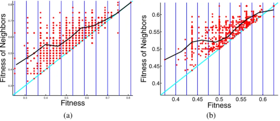
Empirical results for the royal trees are not shown here for lack of space. Nevertheless, they can be found in [17] and they confirm the consistency of the nsc as an hardness indicator. Results for the multiplexer problem are summarized by figures 1(a) and 1(b) and by table 1. Figure 1(a) as well as the first row in table 1 concern the 6 multiplexer problem. For this instance of the problem, performance (p) of GP using only standard mutation as a genetic operator is equal to 0.58 (which means that a global optimum has been found in 58 runs over 100 before generation 500). Given that p is larger than 0.5, this problem can be considered as an “easy” one for GP (even though, being the value of p so close to 0.5, the term “uncertain” would probably be more appropriate). On the
0.3 0.4 0.5 0.6 0.7 0.8 0.3 0.4 0.5 0.6 0.7 0.8 Fitness Fitness of Neighbors 0.4 0.45 0.5 0.55 0.6 0.4 0.45 0.5 0.55 0.6 Fitness Fitness o f Neighbors (a) (b)
Fig. 1. Multiplexer problem, fitness cloud and segments. (a): 6 multiplexer. (b): 11 multiplexer. Table 1. Multiplexer. Indicators related to scatterplots of figure 1.
scatterplot problem p nsc Fig. 1(a) 6 multiplexer 0.58 -0.16 Fig. 1(b) 11 multiplexer 0 -0.24
0.4 0.45 0.5 0.55 0.6 0.65 0.4 0.45 0.5 0.55 0.6 0.65 Fitness Fitness of Neighbors
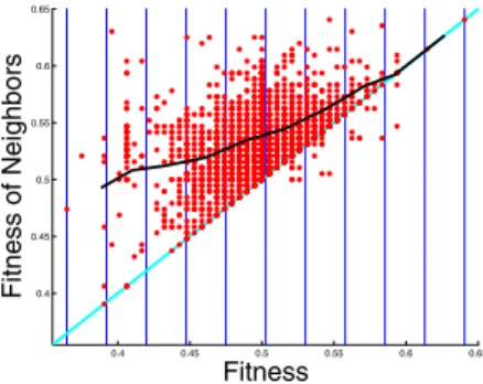
Fig. 2. Intertwined Spirals Problem. Fitness cloud with segments.
Table 2. Intertwined Spirals Problem. Indicators related to the scatterplot of figure 2.
scatterplot problem p nsc Fig. 2 intertwined spirals 0 0
other hand, the value of the nsc is equal to -0.16, which means that, according to the nsc measure, the 6 multiplexer problem should be difficult to solve. Thus, the nsc does not give the correct indication about the hardness of this problem.
Figure 1(b) and the second row of table 1 concern the 11 multiplexer problem. For this instance of the problem, no global optimum has been found by GP using mutation over the 100 runs performed. Thus the problem is clearly difficult and, consistently, nsc has a negative value.
The intertwined spirals problem is difficult to solve by GP. In fact, no optimum has been found over 100 runs. On the other hand, as shown by figure 2 and table 2, the nsc value is equal to zero, which means that, according to the nsc measure, the problem should be easy. While the lack of reliability of the nsc reported in the case of the 6 mul-tiplexer problem could eventually be considered as “marginal”, since GP performance in that case is very close to 0.5 (and thus hardness is very difficult to measure), the wrong indication on the intertwined spirals problem leaves no room for doubts: the nsc, as it has been used in [18] and until now in this paper, cannot be used as a general hard-ness indicator for GP. Thus, the next sections are dedicated to the definition of a new technique for partitioning fitness clouds into segments, in order to assure a higher sta-tistical significance to the set of points belonging to each segment. Successively, some new empirical results are shown, confirming that the new partitioning technique allows to overcome the nsc drawbacks presented here.
5
Size Driven Bisection
One of the most natural ways to automatically partition a fitness cloud into a set of segments consists in applying the well-known bisection algorithm: as a first step, the fitness cloud may be partitioned into two segments, each one containing the same num-ber of points; then the algorithm may be recursively applied to each one of these two
segments until at least one of the segments contains a smaller number of points than a prefixed threshold. This technique has been tested and it has a major drawback: let the size of a segment be defined as the difference between the rightmost and the leftmost abscissas of that segment. After a few number of steps, very small bins (i.e. bins with a very small size) may be generated (see [17], at page 162, for a practical case where this problem arises). In such cases, if small segments have negative slopes, the nsc may take very large values (around 106in the example shown in [17], page 162). This is
clearly unacceptable, even in consideration of the fact that all the points included in-side that segments give more or less the same information. In other words, a segment of such a small size is clearly not a significant one. Such a pathologic situation man-ifests very often if the bisection strategy is applied [17]. Thus, a different strategy is needed.
In an informal way, one may say that the arbitrary criteria used in [18] and in section 4 took into account the size of the segments, but not the number of points they contain, while the bisection algorithm does exactly the opposite. In this section, a technique which takes into account both the size of the segments and the number of points they contain, called size driven bisection for brevity, is proposed. The starting point of this algorithm is the same as for bisection: the fitness cloud is partitioned into two segments, each of which contains the same number of points. After that, instead of recursively applying bisection to both these segments, only the segment with larger size is further partitioned. Partition is done, once again, by bisection, i.e. the segment is partitioned into two bins, each one containing the same number of points. The algo-rithm is iterated until one of the two following conditions is satisfied: either a segment contains a smaller number of points than a prefixed threshold, or a segment has become smaller than a prefixed minimum size. In this paper, as a first approximation, 50 has been chosen as a threshold for the number of points belonging to a bin, and the 5% of the distance between the leftmost and the rightmost points in the fitness cloud has been chosen as the minimum size of a segment.
5.1 Experimental Results
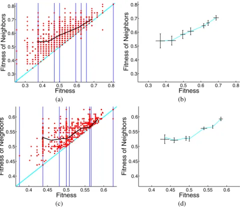
Empirical results for the multiplexer problem using size driven bisection are summa-rized by figures 3 and table 3. Figure 3(a) and figure 3(b) as well as the first row in table 3 concern the 6 multiplexer problem. This time, the value of the nsc is equal to 0 and this value is consistent with the fact that GP performance is > 0.5. Neverthe-less, figure 3(b) (containing standard deviations of the same points as in figure 3(a)) shows that the slope of some segments is not statistically significant. Our interpretation of it is that, since the GP performance value is near 0.5, it is difficult to state if the problem is “easy” or “hard”. We could informally say that it is “moderatedly easy” or maybe “uncertain” and the standard deviations of some segments seem to confirm this “uncertainty”.
Figures 3(c) and 3(d) and the second row of table 3 concern the 11 multiplexer problem. The nsc calculated with the size driven bisection has a negative value and, this time, standard deviations leave few chances to segment slopes to change. In conclusion, nsc using size driven bisection seems a reasonable hardness indicator for the multiplexer problem.
0.3 0.4 0.5 0.6 0.7 0.8 0.3 0.4 0.5 0.6 0.7 0.8 Fitness Fitness of Neighbors 0.3 0.4 0.5 0.6 0.7 0.8 0.3 0.4 0.5 0.6 0.7 0.8 Fitness Fitness of Neighbors (a) (b) 0.4 0.45 0.5 0.55 0.6 0.4 0.45 0.5 0.55 0.6 Fitness Fitness o f Neighbors 0.4 0.45 0.5 0.55 0.6 0.4 0.45 0.5 0.55 0.6 Fitness Fitness o f Neighbors (c) (d)
Fig. 3. Multiplexer problem. (a): 6 multiplexer, fitness cloud and segments. (b): 6 multiplexer,
segments with standard deviations. (c): 11 multiplexer, fitness cloud and segments. (d): 11 multi-plexer, segments with standard deviations.
Table 3. Multiplexer. Indicators related to scatterplots of figure 3.
scatterplot problem p nsc Fig. 3(a) and (b) 6 multiplexer 0.58 0 Fig. 3(c) and (d) 11 multiplexer 0 -0.21
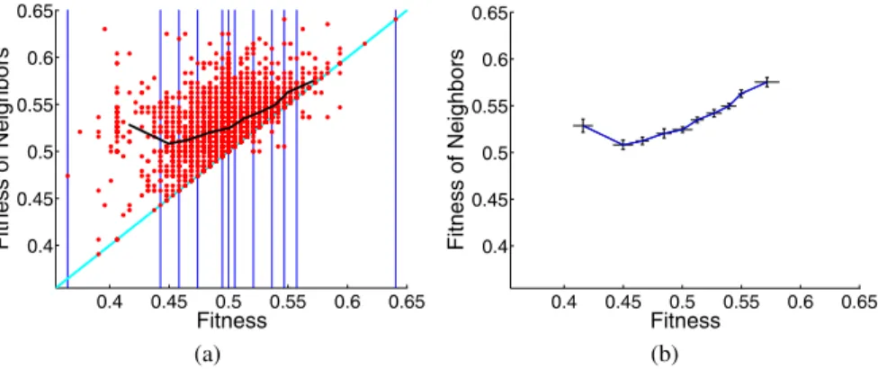
Figure 4 shows the scatterplot and segments with their standard deviations for the intertwined spirals problem. Table 4 shows that the value of the nsc calculated using size driven bisection is negative. Standard deviations confirm that all the segment slopes are statistically significant. We conclude that nsc gives reasonable indications on the hardness of this problem too.
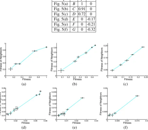
Finally, figures 5(a), 5(b) and 5(c) show the scatterplot and segments for the royal tree problem in the case where
F
={A,B},F
={A,B,C}F
={A,B,C,D}. In thesecases, performance values (p) confirm that the problem is easy for GP. The first three rows of table 5 show that nsc is equal to zero in all these cases. Furthermore (see figures 6(a), 6(b) and 6(c)) standard deviations confirm that all the segment slopes are statistically significant. On the other hand, if E, F and G nodes are added to the set
0.4 0.45 0.5 0.55 0.6 0.65 0.4 0.45 0.5 0.55 0.6 0.65 Fitness Fitne ss of Neigh b or s 0.4 0.45 0.5 0.55 0.6 0.65 0.4 0.45 0.5 0.55 0.6 0.65 Fitness Fitne ss of Neigh b or s (a) (b)
Fig. 4. Intertwined Spirals Problem. (a) : Fitness cloud with segments. (b) : Segments with
stan-dard deviations.
Table 4. Intertwined Spirals. Indicators related to scatterplots of figure 4.
scatterplot problem p nsc Fig. 4(a) and (b) intertw. spirals 0 -0.41
0 0.2 0.4 0.6 0.8 1 0 0.2 0.4 0.6 0.8 1 Fitness Fitne ss of Neigh b or s 0 0.1 0.2 0.3 0.4 0.5 0.6 0 0.1 0.2 0.3 0.4 0.5 0.6 Fitness Fitne ss of Neigh b or s 0 0.05 0.1 0.15 0.2 0.25 0 0.05 0.1 0.15 0.2 0.25 Fitness Fitne ss of Neigh b or s (a) (b) (c) 0 0.02 0.04 0.06 0.08 0 0.01 0.02 0.03 0.04 0.05 0.06 0.07 0.08 Fitness Fitne ss of Neigh b or s 0 0.01 0.02 0.03 0 0.005 0.01 0.015 0.02 0.025 0.03 0.035 Fitness Fitne ss of Neigh b or s 0 0.005 0.01 0.015 0.02 0 0.005 0.01 0.015 0.02 Fitness Fitne ss of Neigh b or s (d) (e) (f)
Fig. 5. Royal tree problem. Fitness clouds with segments. (a): F = {A,B}. (b): F =
{A,B,C}. (c): F ={A,B,C,D}. (d): F = {A,B,C,D,E}. (e): F = {A,B,C,D,E,F}. (f): F ={A,B,C,D,E,F,G}. Note the change in the axis scale as theF set increases in size. of possible function nodes, the problem becomes difficult (since performance is equal to zero, as shown by the last three rows of table 5). Consistently, the nsc becomes more and more negative for these instances of the problem. Figures 5(d), 5(e) and 5(f) show scatterplots and segments for these three instances and figures 6(d), 6(e) and 6(f) show
Table 5. Royal trees. Some data related to scatterplots of figure 5. scatterplot root p nsc Fig. 5(a) B 1 0 Fig. 5(b) C 0.91 0 Fig. 5(c) D 0.72 0 Fig. 5(d) E 0 -0.17 Fig. 5(e) F 0 -0.21 Fig. 5(f) G 0 -0.32 0 0.2 0.4 0.6 0.8 1 0 0.2 0.4 0.6 0.8 1 Fitness Fitne ss of Neigh b or s 0 0.1 0.2 0.3 0.4 0.5 0.6 0 0.1 0.2 0.3 0.4 0.5 0.6 Fitness Fitne ss of Neigh b or s 0 0.05 0.1 0.15 0.2 0.25 0 0.05 0.1 0.15 0.2 0.25 Fitness Fitne ss of Neigh b or s (a) (b) (c) 0 0.02 0.04 0.06 0.08 0 0.01 0.02 0.03 0.04 0.05 0.06 0.07 0.08 Fitness Fitne ss of Neigh b or s 0 0.01 0.02 0.03 0.04 0 0.005 0.01 0.015 0.02 0.025 0.03 0.035 0.04 Fitness Fitne ss of Neigh b or s 0 0.005 0.01 0.015 0.02 0 0.005 0.01 0.015 0.02 Fitness Fitne ss of Neigh b or s (d) (e) (f)
Fig. 6. Royal tree problem. Segments with standard deviations. (a): F ={A,B}. (b): F =
{A,B,C}. (c):F ={A,B,C,D}. (d):F ={A,B,C,D,E}. (e):F ={A,B,C,D,E,F}. (f):F =
{A,B,C,D,E,F,G}. Note the change in the axis scale as theF set increases in size.
the respective standard deviations. Once again, nsc values correctly indicate the relative order of GP problem hardness.
6
Conclusions and Future Work
The negative slope coefficient (nsc) is not a reliable measure of problem hardness if the fitness cloud is partitioned into segments in an arbitrary way. In this paper, a new way of partitioning fitness clouds, called size driven bisection, has been presented. It represents a suitable tradeoff between the size of segments and the density of points in the partitions. The nsc using size driven bisection gave reliable indications about the hardness of two instances of the multiplexer problem, the intertwined spirals problem and six instances of the royal trees problem. Furthermore, the nsc using size driven bisection gave reliable indications on some other typical GP benchmarks (such as the artificial ant on the Santa Fe trail, the even parity and one particular instance of the
symbolic regression) and on trap functions (these results have not been shown here for lack of space. They are presented in [17]). These results encourage us to continue the study of nsc, with further tests on more “real life” GP problems. This paper leaves some open problems: first of all, it is based on statistical samplings of the search space and thus counterexamples can surely be built for this measure. Furthermore, and even more importantly, no technique has been found yet to normalize nsc values into a given range, in order to enable comparisons between the difficulties of two or more problems of different nature. Only the hardness of different instances of the same problem can be calculated using nsc, as defined here.
References
1. L. Altenberg. The evolution of evolvability in genetic programming. In K. Kinnear, editor, Advances in Genetic Programming, pages 47–74, Cambridge, MA, 1994. The MIT Press. 2. M. Clergue, P. Collard, M. Tomassini, and L. Vanneschi. Fitness distance correlation and
problem difficulty for genetic programming. In et al. W. B. Langdon, editor, Proceedings of the Genetic and Evolutionary Computation Conference, GECCO’02, pages 724–732, New York City, USA, 2002. Morgan Kaufmann, San Francisco, CA.
3. K. Deb and D. E. Goldberg. Analyzing deception in trap functions. In D. Whitley, editor, Foundations of Genetic Algorithms, 2, pages 93–108. Morgan Kaufmann, 1993.
4. S. Forrest and M. Mitchell. What makes a problem hard for a genetic algorithm? some anomalous results and their explanation. Machine Learning, 13:285–319, 1993.
5. J. Horn and D. E. Goldberg. Genetic algorithm difficulty and the modality of the fitness landscapes. In D. Whitley and M. Vose, editors, Foundations of Genetic Algorithms, 3, pages 243–269. Morgan Kaufmann, 1995.
6. T. Jones. Evolutionary Algorithms, Fitness Landscapes and Search. PhD thesis, University of New Mexico, Albuquerque, 1995.
7. K. E. Kinnear Jr. Fitness landscapes and difficulty in genetic programming. In Proceed-ings of the First IEEEConference on Evolutionary Computing, pages 142–147. IEEE Press, Piscataway, NY, 1994.
8. J. R. Koza. Genetic Programming. The MIT Press, Cambridge, Massachusetts, 1992. 9. W. B. Langdon and R. Poli. Foundations of Genetic Programming. Springer, Berlin,
Heidel-berg, New York, Berlin, 2002.
10. N. Madras. Lectures on Monte Carlo Methods. American Mathematical Society, Providence, Rhode Island, 2002.
11. B. Manderick, M. de Weger, and P. Spiessens. The genetic algorithm and the structure of the fitness landscape. In R. K. Belew and L. B. Booker, editors, Proceedings of the Fourth International Conference on Genetic Algorithms, pages 143–150. Morgan Kaufmann, 1991. 12. M. Mitchell, S. Forrest, and J. Holland. The royal road for genetic algorithms: fitness land-scapes and ga performance. In F. J. Varela and P. Bourgine, editors, Toward a Practice of Autonomous Systems, Proceedings of the First European Conference on Artificial Life, pages 245–254. The MIT Press, 1992.
13. B. Naudts and L. Kallel. A comparison of predictive measures of problem difficulty in evolutionary algorithms. IEEE Transactions on Evolutionary Computation, 4(1):1–15, 2000. 14. W. Punch. How effective are multiple populations in genetic programming. In J. R. Koza, W. Banzhaf, K. Chellapilla, K. Deb, M. Dorigo, D. B. Fogel, M. Garzon, D. Goldberg, H. Iba, and R. L. Riolo, editors, Genetic Programming 1998: Proceedings of the Third Annual Con-ference, pages 308–313, San Francisco, CA, 1998. Morgan Kaufmann.
15. P. F. Stadler. Fitness landscapes. In M. L¨assig and Valleriani, editors, Biological Evolu-tion and Statistical Physics, volume 585 of Lecture Notes Physics, pages 187–207. Springer, Berlin, Heidelberg, New York, 2002.
16. M. Tomassini, L. Vanneschi, P. Collard, and M. Clergue. A study of fitness distance cor-relation as a difficulty measure in genetic programming. Evolutionary Computation, 13(2): 213–239, 2005.
17. L. Vanneschi. Theory and Practice for Efficient Genetic Programming. Ph.D. thesis, Faculty of Science, University of Lausanne, Switzerland, 2004. Downlodable version at: http://www.disco.unimib.it/vanneschi.
18. L. Vanneschi, M. Clergue, P. Collard, M. Tomassini, and S. V´erel. Fitness clouds and prob-lem hardness in genetic programming. In K. Deb et al., editor, Proceedings of the Genetic and Evolutionary Computation Conference, GECCO’04, volume 3103 of Lecture Notes in Computer Science, pages 690–701. Springer, Berlin, Heidelberg, New York, 2004.
19. L. Vanneschi, M. Tomassini, M. Clergue, and P. Collard. Difficulty of unimodal and multi-modal landscapes in genetic programming. In Cant´u-Paz, E., et al., editor, Proceedings of the Genetic and Evolutionary Computation Conference, GECCO’03, LNCS, pages 1788–1799, Chicago, Illinois, USA, 2003. Springer, Berlin, Heidelberg, New York.
20. L. Vanneschi, M. Tomassini, P. Collard, and M. Clergue. Fitness distance correlation in genetic programming: a constructive counterexample. In Congress on Evolutionary Compu-tation (CEC’03), pages 289–296, Canberra, Australia, 2003. IEEE Press, Piscataway, NJ. 21. S. V´erel, P. Collard, and M. Clergue. Where are bottleneck in nk-fitness landscapes ? In
CEC 2003: IEEE International Congress on Evolutionary Computation. Canberra, Aus-tralia, pages 273–280. IEEE Press, Piscataway, NJ, 2003.
22. E. D. Weinberger. Correlated and uncorrelated fitness landscapes and how to tell the differ-ence. Biol. Cybern., 63:325–336, 1990.