HAL Id: hal-02376158
https://hal.inria.fr/hal-02376158
Submitted on 22 Nov 2019
HAL is a multi-disciplinary open access
archive for the deposit and dissemination of
sci-entific research documents, whether they are
pub-lished or not. The documents may come from
teaching and research institutions in France or
abroad, or from public or private research centers.
L’archive ouverte pluridisciplinaire HAL, est
destinée au dépôt et à la diffusion de documents
scientifiques de niveau recherche, publiés ou non,
émanant des établissements d’enseignement et de
recherche français ou étrangers, des laboratoires
publics ou privés.
Reversing Unbounded Petri Nets
Lukasz Mikulski, Ivan Lanese
To cite this version:
Lukasz Mikulski, Ivan Lanese. Reversing Unbounded Petri Nets. PETRI NETS 2019 -
Applica-tions and Theory of Petri Nets, Jun 2019, Aachen, Germany. �10.1007/978-3-030-21571-2_13�.
�hal-02376158�
Łukasz Mikulski1 and Ivan Lanese2
1
Folco Team, Nicolaus Copernicus University [email protected]
2
Focus Team, University of Bologna/INRIA [email protected]
Abstract. In Petri nets, computation is performed by executing
transi-tions. An effect-reverse of a given transition b is a transition that, when executed, undoes the effect of b. A transition b is reversible if it is possi-ble to add enough effect-reverses of b so to always being apossi-ble to undo its effect, without changing the set of reachable markings.
This paper studies the transition reversibility problem: in a given Petri net, is a given transition b reversible? We show that, contrarily to what happens for the subclass of bounded Petri nets, the transition reversibil-ity problem is in general undecidable. We show, however, that the same problem is decidable in relevant subclasses beyond bounded Petri nets, notably including all Petri nets which are cyclic, that is where the ini-tial marking is reachable from any reachable marking. We finally show that some non-reversible Petri nets can be restructured, in particular by adding new places, so to make them reversible, while preserving their behaviour.
Keywords: Petri Nets, reverse transition, reversibility
1
Introduction
Reversible computation, a computational paradigm where any action can be undone, is attracting interest due to its applications in fields as different as low-power computing [24], simulation [9], robotics [27] and debugging [29]. Re-versible computation has been explored in different settings, including digital circuits [32], programming languages [33,26], process calculi [12], and Turing machines [5]. In this paper, we focus on reversible computation in the setting of Petri nets.
In the early years of investigation of Petri nets (the seventies), a notion of local reversibility [8,19], requiring each transition to have a reverse transition, was used. The reverse b−of a transition b undoes the effect of b in any marking (i.e., in any state) reachable by executing b. That is, after having executed b from some marking M it is always possible to execute b−, and this leads back to marking M . Local reversibility is close to the definition currently used in, e.g., process calculi [12], programming languages [33,26] and Turing machines [5]. As
?This work has been partially supported by COST Action IC1405 on Reversible
Computation - extending horizons of computing. The second author has been also partially supported by French ANR project DCore ANR-18-CE25-0007.
time passed, a notion of global reversibility [15], requiring the initial state to be reachable by any reachable state of the net, attracted more interest because of its applications in controllability enforcing [23,31] and reachability testing [28]. The notion of local reversibility occurred for some time under the name of symmetric Petri nets [15], however, this name later changed the meaning to denote other forms of state space symmetry [21,10]. In this paper, with reversibility we mean a form of local reversibility (detailed below), and following [7] we write cyclicity to refer to the other notion. In order to relate reversibility and cyclicity, one would like to understand whether a Petri net can be made cyclic by adding reverse transitions or, more generally, whether reverse transitions can be added.
This problem was first tackled in [2] for the restricted class of bounded Petri nets. They provided the main insight below: the main issue is that adding reverse transitions must not change the behaviour of the net, which was defined as the set of reachable markings. However, this happens if the reverse of a transition b can trigger also in a marking not reachable by executing b as last transition, hence reverse transitions cannot always be added. However, in bounded Petri nets one can always add a complete set of effect-reverses. An effect-reverse of a transition b is a transition that, when executed, has the same effect as the reverse of b. However, an effect-reverse may not be enabled in all the markings the reverse is, hence adding one effect-reverse is in general not enough. A set of effect-reverses able to reverse a given transition b in all the markings where the reverse b− can do it is called complete.
Hence, following [2], we define the transition reversibility problem as follows: in a given Petri net, can we add a complete set of effect-reverses for a given transition b without changing the set of reachable markings? We say a net is re-versible if the answer to the transition reversibility problem is positive for each transition. The approach in [2] cannot be easily generalised to cope with un-bounded Petri nets. The problem is hard in the unun-bounded case (indeed, we will show it to be undecidable) since adding even a single reverse (or effect-reverse) transition can have a great, and not easily characterisable, impact on the net. Indeed, the problem MESTR (Marking Equality with Single Transition Reverse) of establishing whether adding a single reverse (or effect-reverse) transition to a given net changes the set of reachable markings is, in general, undecidable [3]. One can, however, try to add effect-reverses, hoping to get a complete set of them without needing the ones for which the MESTR problem is undecidable.
In this paper, we tackle the transition reversibility problem in nets which are not necessarily bounded. We propose an approach based on identifying pairs of markings which forbid to add the effect-reverses of a specific transition b (Section 3). We call such pairs b-problematic. We show that a transition b is reversible iff there is no b-problematic pair (Corollary 1). We then study relevant properties of b-problematic pairs, including decidability and complexity issues (Section 4). In particular, we show that the existence of b-problematic pairs is undecidable (Theorem 3), which is surprising since for a given transition b the set of minimal b-problematic pairs is finite (Proposition 2), and checking whether a given pair of markings is b-problematic is decidable (Corollary 2).
Given that the problem is undecidable, we identify relevant subclasses of Petri nets where the problem becomes decidable (Section 5). We show, in particular, that cyclicity implies reversibility (Corollary 3), which in our opinion provides a novel link between the two notions.
In order to have more reversible nets, we study whether a net can be re-structured so to make it reversible while preserving its behaviour, in the sense described below (Section 6). First, we show that some nets, but not all, can be made reversible by extending them with new places, while preserving the re-quirements and effect of transitions on existing ones. Second, we consider whether the reversed behaviour of a net (obtained by considering the net as a labelled transition system and then adding reverse transitions) could be obtained as a behaviour of any Petri net, possibly completely different from the starting one. Surprisingly, this is possible only for Petri nets that can be made reversible by just extending them with new places (Theorem 5).
2
Background
In this section we introduce the notions needed for our developments. While these are largely standard, we mainly follow the presentation from [2] and [4].
The group ZX
and the monoid NX
The set of all integers is denoted by Z, while the set of non-negative integers by N. Given a set X, the cardinality (number of elements) of X is denoted by |X|, the powerset (set of all subsets) by 2X. Multisets over X are members of
NX, i.e., functions from X into N. We extend the notion for all integers in an intuitive way obtaining mappings from X into Z. If the set X is finite, mappings from X into Z (as well as N) will be represented by vectors of Z|X|, written as [x1, . . . , x|X|] (assuming a fixed ordering of the set X). Given a function f we
represent its domain restriction to a set X (subset of its domain) as f ↓X.
The group ZX, for a set X, is the set of mappings from X into Z with componentwise addition + (note that NX with + is a monoid). If Y, Z ∈ ZX then (Y + Z)(x) = Y (x) + Z(x) for every x ∈ X, while for A, B ⊆ ZX we have A + B = {Y + Z | Y ∈ A ∧ Z ∈ B}. We define subtraction, denoted by −, analogously. The star operation is defined as Y∗ =S{Yi | i ∈ N}, where Y0 is
a constant function equal 0 for every argument, denoted by 0, and Yi+1 = Yi+Y .
Rational subsets of NX
are subsets built from atoms (single elements of NX) with
the use of finitely many operations of union ∪, addition + and star∗. The partial order ≤ (both on mappings and tuples) is understood componentwise, while < means ≤ and 6=. Given A ⊆ ZX, min(A) is the set of minimal elements in A.
For tuples over X we define first : Xn→ X by first ((x
1, x2, . . . , xn)) = x1.
Transition systems
A labelled transition system (or, simply, lts) is a tuple T S = (S, T, →, s0) with a
set of states S, a finite set of labels T , a set of arcs → ⊆ (S ×T ×S), and an initial state s0∈ S. We draw an lts as a graph with states as nodes, and labelled edges
defined by arcs. A label a is fireable at s ∈ S, denoted by s[ai, if (s, a, s0) ∈ →, for some s0∈ S. A state s0is reachable from s through the execution of a sequence of
transitions σ ∈ T∗, written s[σis0, if there is a directed path from s to s0 whose arcs are labelled consecutively by σ. A state s0is reachable if it is reachable from the initial state s0. The set of states reachable from s is denoted by [si. A state
s0 is reachable by a (also said a-reachable) if it is reachable via a sequence of transitions having a as last element. A sequence σ ∈ T∗ is fireable, from a state s, denoted by s[σi, if there is some state s0such that s[σis0. A labelled transition system T S = (S, T, →, s0) is called finite if the set S is finite.
We assume that for each a ∈ T , the set of arcs labelled by a is nonempty. Let T S1= (S1, T, →1, s01) and T S2 = (S2, T, →2, s02) be ltss. A total
func-tion ζ : S1 → S2 is a homomorphism from T S1 to T S2 if ζ(s01) = s02 and
(s, a, s0) ∈ →1⇔ (ζ(s), a, ζ(s0)) ∈ →2, for all s, s0∈ S1, a ∈ T . T S1 and T S2 are
isomorphic if ζ is a bijection.
Petri nets
A Place/Transition Petri net (or, simply, net ) is a tuple N = (P, T, F, M0),
where P is a finite set of places, T is a finite set of transitions, F is the flow function F : ((P × T ) ∪ (T × P )) → N specifying the arc weights, and M0is the
initial marking. Markings are mappings M : P → N.
Petri nets admit a natural graphical representation (see, e.g., net N1in
Fig-ure 1 of Section 3). Nodes represent places and transitions, arcs represent the weight function (we drop the weight if it is 1). Places are indicated by circles, and transitions by boxes. Markings are depicted by tokens inside places.
The effect of a transition a on a place p is effp(a) = F (a, p) − F (p, a). The (total) effect of transition a ∈ T is a mapping eff (a) : P → Z, where eff (a)(p) = effp(a) for every p ∈ P . For a transition a ∈ T we define two mappings: ena,
called entries, and exa, called exits, as follows: ena, exa: P → N and ena(p) =
F (p, a) as well as exa(p) = F (a, p) for every p ∈ P . A transition a ∈ T is enabled
at a marking M , denoted by M [ai, if M ≥ ena. The firing of a at marking M
leads to M0, denoted by M [aiM0, if M [ai and M0 = M + eff (a) (note that there is no upper limit to the number of tokens that a place can hold). The notions of enabledness and firing, M [σi and M [σiM0, are extended in the usual way to sequences σ ∈ T∗, and [M i denotes the set of all markings reachable from M . We assume that each transition is enabled in at least one reachable marking. It is easy to observe that transition enabledness is monotonic: if a transition a is enabled at marking M and M ≤ M0, then a is also enabled at M0.
Note that markings as well as entries and exits of a transition are multisets over P (mappings from P to N), while total effect is a mapping from P to Z, hence we represent all of them as vectors (after fixing an order on P ).
The reachability graph of a Petri net N = (P, T, F, M0) is defined as the lts
RG(N ) = ([M0i, T, {(M, a, M0) | M, M0∈ [M0i ∧ M [aiM0}, M0).
Intuitively, the reachability graph has reachable markings as states and firings as arcs. If a labelled transition system T S is isomorphic to the reachability graph of a Petri net N , then we say that N solves T S, and T S is synthesisable to N . A Petri net N = (P, T, F, M0) is bounded if [M0i is finite (hence its reachability
if there exists np∈ N such that M(p) < np for every M ∈ [M0i, otherwise the
place is unbounded. The set of all bounded places of the net N is denoted by bound (N ). Note that every place of a bounded net is bounded, while in each unbounded net there exists at least one unbounded place.
We now define reverses of transitions, and effect-reverses of transitions.
Definition 1 (transition reverse and effect-reverse). The reverse of a
transition a ∈ T in a net N = (P, T, F, M0) is the transition a− such that for
each p ∈ P we have F (p, a−) = F (a, p) and F (a−, p) = F (p, a). An effect-reverse of a transition a ∈ T is any transition a−e such that eff (a−e) = −eff (a).
A minimum effect-reverse (that is, an effect-reverse without self-loops) of a transition a ∈ T is a transition a−esuch that for each p ∈ P we have ena−e(p) =
−effp(a−e) and exa−e(p) = 0 if effp(a−e) ≤ 0, and ena−e(p) = 0 and exa−e(p) =
effp(a−e) otherwise.
Notably, the reverse of a transition is also an effect-reverse, but not every effect-reverse is a reverse. Furthermore, a reverse of a transition a is able to reverse the transition a in any marking reachable by a, while an effect-reverse may do it only in some of these markings. A set of effect-reverses for transition a is complete if it includes enough effect-reverses to reverse a at any marking reachable by a.
We now define the notions of reversibility and cyclicity we are interested in.
Definition 2 (reversibility). A transition b is reversible in a net N if it is
possible to add to N a complete set of effect-reverses of b without changing the set of reachable markings. A net N is reversible if all its transitions are reversible.
Definition 3 (cyclicity). Let N = (P, T, F, M0) be a Petri net. A marking M
reachable in N is called a home state if it is reachable from any other marking reachable in N . A net N is cyclic if M0 is a home state.
3
Problematic pairs
In this paper, we tackle the transition reversibility problem, that is we want to decide whether, in a given Petri net N (possibly unbounded), we can add a complete set of effect-reverses of a given transition b without changing the set of reachable markings. In other words, if N is the original net and N0 the one obtained by adding the complete set of effect-reverses, then their reachability graphs RG(N ) and RG(N0) differ only for the presence of reverse transitions in RG(N0). In particular, no new markings are reachable in N0, hence RG(N ) and
RG(N0) have the same set of states.
We remark that the net obtained by adding complete sets of effect-reverses for each transition (without changing the set of reachable markings) is by con-struction reversible and also trivially cyclic, hence understanding the transition reversibility problem is the key for understanding also reversibility and cyclicity. In this section we show that the transition reversibility problem for transition b is equivalent to deciding the absence of particular pairs of markings, that we
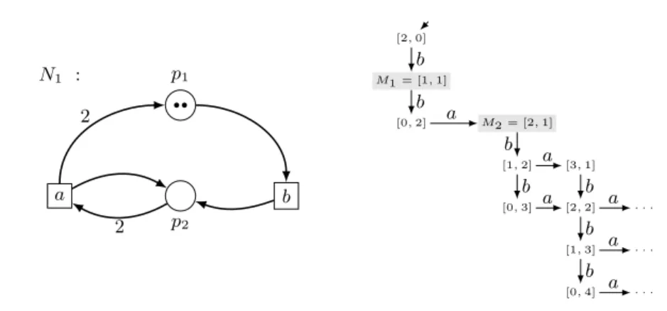
N1 : p2 p1 a b •• 2 2 [2, 0] M1 = [1, 1] [0, 2] M2 = [2, 1] [1, 2] [0, 3] [3, 1] [2, 2] [1, 3] [0, 4] . . . . . . . . . b b a b b a b b b a a a a
Fig. 1. A Petri net N1 and part of its reachability graph (transition system).
call b-problematic, introduced below. This characterisation will help us in solving the transition reversibility problem for relevant classes of Petri nets.
Let us start by considering the sample net N1 in Figure 1. Net N1 has two
unbounded places, hence the theory from [2], valid for bounded nets, does not apply. Furthermore, adding a complete set of effect-reverses for transition b in net N1changes the set of reachable markings. Intuitively, the reason is that the
net contains two markings M1and M2such that in M1at least one effect-reverse
should trigger, in M2 it must not (since M2 is not reachable by b), but M2 is
greater than M1. Hence, by monotonicity, we have a contradiction.
We now introduce the notion of b-problematic pair to formalise the intuition.
Definition 4 (b-problematic pair). Let N = (P, T, F, M0) be a net, and b ∈ T
a transition. A pair (M1, M2) of markings reachable in N is b-problematic if
M1< M2, ∃σ∈T∗M0[σbiM1 and ∀ρ∈T∗¬M0[ρbiM2.3
The set of all b-problematic pairs in N is denoted by Pb(N ).
We say a pair is problematic if it is b-problematic for some transition b. Pair ([1, 1], [2, 1]) is b-problematic in net N1in Figure 1. Intuitively, an
effect-reverse of b should trigger in marking [1, 1] (reachable by b) but not in marking [2, 1] (not reachable by b), but monotonicity forbids this.
The notion of problematic pair has been also implicitly used by [7], to define the notion of complete Petri net and study the inverse of a Petri net. Complete-ness allows one to block reverse transitions in all markings that do not occur as second component of a problematic pair.
We can now prove that b-problematic pairs forbid to reverse transition b.
Proposition 1. Let N = (P, T, F, M0) be a Petri net and b ∈ T a transition. If
there exists in N a b-problematic pair, then b is not reversible in N . 3
Note that there can be two reasons for ¬M0[ρbiM2. Either ρb is not enabled at M0
Proof. Let (M1, M2) be the b-problematic pair. A complete set of effect-reverses
should include at least one effect-reverse b−e triggering in M1. By monotonicity
b−etriggers also in M2, but, since M2 is not reachable by b, adding b−e changes
the set of reachable markings. This proves the thesis. ut
The result above is independent of the number of effect-reverses in the com-plete set, hence even considering an infinite set of effect-reverses would not help. We have shown that the existence of b-problematic pairs implies that b is not reversible. We now prove the opposite implication, namely that absence of b-problematic pairs implies reversibility of b.
Theorem 1. Let N = (P, T, F, M0) be a Petri net and b ∈ T a transition. If no
b-problematic pair exists in N , then b is reversible in N .
Proof. Take a reachable marking M . If it is greater than a b-reachable marking then it is b-reachable (otherwise we would obtain a b-problematic pair). Take the set bR of b-reachable markings. Let min(bR) be the set of all minimal elements in bR. They are all incomparable, hence by Dickson’s Lemma [14] the set min(bR) is finite. Let us consider the set of effect-reverses of b composed of the effect-reverses b−eof b such that enb−e ∈ min(bR). Note that we have one such effect-reverse for
each marking in min(bR). By monotonicity, we have at least one effect-reverse triggering at each marking in bR, and no effect-reverse triggering outside bR, hence this is a complete set of effect-reverses (that do not change the set of
reachable markings) as desired. ut
The result above is an unbounded version of the procedure presented in the proof of [2, Theorem 4.3] for bounded nets. By combining the two results above we get the following corollary, showing that b-problematic pairs provide an equivalent formulation of the transition reversibility problem.
Corollary 1. Let N = (P, T, F, M0) be a Petri net and b ∈ T a transition. The
transition b is reversible in N iff no b-problematic pair exists in N .
The formulation in terms of b-problematic pairs raises the following question:
– Is it decidable whether a b-problematic pair exists in a given net?
In Section 4 we answer negatively the question above, hence the transition re-versibility problem is in general undecidable. This raises additional questions:
1. Can we decide whether a given pair of markings is b-problematic for a net? 2. Can we find relevant classes of nets where the transition reversibility problem
is decidable?
3. Can we transform a net into a reversible one while preserving its behaviour? We will answer the questions above in Sections 4, 5 and 6, respectively.
4
Undecidability of the existence of b-problematic pairs
The main result of this section is the undecidability of the existence of b-problematic pairs and, as a consequence, of the transition reversibility problem. Before proving our main result we show, however, that a given net has finitely many minimal b-problematic pairs, and that one can decide (indeed it is equivalent to the Reachability Problem) whether a given pair of markings is b-problematic. These results combined seem to hint at the decidability of the transition reversibility problem. However, this is not the case.
We start by proving that there are finitely many minimal b-problematic pairs.
Proposition 2. Let N = (P, T, F, M0) be a net, and b ∈ T a transition. There
exist finitely many minimal b-problematic pairs in N .
Proof. A b-problematic pair ([x1, . . . , xn], [y1, . . . , ym]) can be seen as a tuple
(x1, . . . , xn, y1, . . . , ym), hence the result follows from Dickson’s Lemma [14]. ut
We now show by reduction to the Reachability Problem that one can decide whether a given pair of markings is b-problematic.
Lemma 1. One can reduce the problem of checking whether a given pair of
markings is b-problematic to the Reachability Problem.
Proof. Let (M1, M2) be the given pair of markings. One has to check that they
are reachable and that the marking M1− eff (b) is reachable, and M2− eff (b) is
not, which are four instances of reachability. ut
On the other hand, we can reduce the Reachability Problem to checking whether a given pair of markings is b-problematic.
Theorem 2. One can reduce the Reachability Problem to the problem of
check-ing whether a given pair of markcheck-ings is b-problematic.
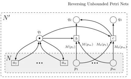
Proof. The proof is by construction. The construction is depicted in Figure 2. Let N = (P, T, W, M0) be a net and M a marking of this net. We will build a new
net N0and a pair of markings (M1, M2) in it such that (M1, M2) is b-problematic
in N0 if and only if M is reachable in N .
We define net N0 as (P ∪ {q1, q2, q3}, T ∪ {b, c}, W0, M00). We assume that
q1, q2, q3, b, c are fresh objects. For the vector representation of markings in N0
we fix the order of places as follows: first the places from N (in the order they have in N ), then places q1, q2, q3 in order. We set M00 = [x1, . . . , xn, 1, 0, 0] with
[x1, . . . , xn] = M0. W0 extends W as follows. Place q1 is connected by a
self-loop with every transition a ∈ T , and a preplace of the two new transitions b, c. Place q2 is a postplace for both new transitions, while q3 is a postplace for c
only. Moreover, c and b take from any place p ∈ P a number of tokens equal to, respectively, M0(p) and M (p).
In the constructed net we can always reach marking M2= [0, . . . , 0, 1, 1] (by
q1 q2 q3 p1 pm b c a1 an • • • • • • • M (p1) M (pm) M0(p1) M0(pm)
N
N
0Fig. 2. Reducing reachability to checking whether a pair of markings is b-problematic.
to place q3, but b and c are in conflict because of place q1). We can also reach
marking M1= [0, . . . , 0, 1, 0] by executing b iff M is reachable in N . Indeed, if b
triggers in some marking M3> M then some tokens are left in the places from N ,
and they are never consumed since b consumes the token in q1, which is needed
to perform any further transition. Thus, the pair (M1, M2) is b-problematic in
N0 if and only if M is reachable in N .
This proves that we can use a decision procedure checking whether a pair of markings is b-problematic in order to solve the Reachability Problem. ut We can combine the two results above to give a precise characterisation of the complexity of checking whether a given pair of markings is b-problematic.
Corollary 2. The problem of deciding whether a given pair of markings is
b-problematic and the Reachability Problem are equivalent.
As a consequence, known bounds for the complexity of the Reachability Prob-lem apply to the probProb-lem of deciding whether a given pair of reachable markings is b-problematic as well. For instance, we know that it is not elementary [11].
At this stage it looks like there should be a procedure to construct the fi-nite set min(Pb(N )). Indeed, we can perform an additional step in this
direc-tion: we can compute a (finite) over-approximation min(Eb(N ) + {eff (b)}) (we
remind that Eb(N ) is the set of markings of N where b is enabled) of the
(fi-nite) set min(first (Pb(N ))) of the minimals of the markings that may occur as
first component in a b-problematic pair. Both the set min(first (Pb(N ))) and its
approximation are finite, but deciding membership and browsing the over-approximation is easy, while even the emptiness problem is actually undecidable for the set min(first (Pb(N ))).
We first need a lemma on monotonicity properties of b-problematic pairs.
Lemma 2. Let N = (P, T, F, M0) be a net, b ∈ T a transition, and (M1, M2) a
– If M3< M1 and ∃σ∈T∗M0[σbiM3 then (M3, M2) is a b-problematic pair.
– If M2 < M4, M4 is reachable and ∀ρ∈T∗¬M0[ρbiM4 then (M1, M4) is a
b-problematic pair.
Proof. Directly from Definition 4, using the transitivity of <. ut We now prove the correctness of our over-approximation.
Lemma 3. Let N = (P, T, F, M0) be a net, b ∈ T a transition. Then:
min(first (Pb(N ))) ⊆ min(Eb(N ) + {eff (b)})
Proof. Take a b-problematic pair (M1, M2). By definition M1 is an element of
Eb(N )+{eff (b)}. Assume it is not minimal. Then there exists M3∈ min(Eb(N )+
{eff (b)}) such that M3 < M1 and so, by Lemma 2, (M3, M2) is also a
b-problematic pair, hence M1∈ min(first (P/ b(N ))). ut
Contrarily to what one could expect from these encouraging preliminary results, the existence of a b-problematic pair is undecidable.
Theorem 3. The problem of the existence of a b-problematic pair is undecidable.
Proof. Assume towards a contradiction that we can decide the existence of a b-problematic pair in a net N . Consider the decision problem MESTR from [3] – Are the reachability sets of two given nets N and N0, where N0 is obtained from N by adding the single reverse b− of a given transition b, equal? We show below that we can reduce MESTR to checking the existence of a b-problematic pair.
Consider the following procedure. If N cannot be reversed by a set of effect-reverses then it cannot be reversed by a single reverse b−. Hence, if there exists a b-problematic pair in N , then the answer for MESTR is negative.
Otherwise we construct the set of markings
X = (NP\ (min(Eb(N ) + eff (b)) + NP)) ∩ (exb+ NP).
X consists of markings ˆM (reachable or not) such that: 1. b− triggers in ˆM ;
2. ˆM is not b-reachable;
Condition 1 holds thanks to (exb+ NP). Condition 2 holds since ˆM is not in the
set (min(Eb(N ) + eff (b)) + NP).
We show now that, if there exists no b-problematic pair in N , then X contains all reachable markings which are not b-reachable. Assume towards a contradiction that M /∈ X is reachable in N but not reachable by b. Then M /∈ min(Eb(N ) + eff (b)) (because it is not reachable by b) and there exists
M0 ∈ min(Eb(N ) + eff (b)) which is smaller than M (because otherwise M ∈ X).
Hence (M0, M ) is a problematic pair which we excluded.
As a result, if there exists no b-problematic pair in N , it is enough to ask, whether there is any reachable marking in X. If one such marking exists then the
answer for MESTR is positive, otherwise it is negative. It remains to show that (i) one can construct the set X and (ii) check whether it contains any marking reachable in N .
To prove part (i) we utilise the fact that (min(Eb(N ) + eff (b)) is finite and
can be easily computed using Dickson’s lemma and the coverability set (see [16]) of N . Moreover, {exb} is a singleton while NP is the set of all multisets over P .
Summing up, NP, (min(Eb(N ) + eff (b)), and exb+ NP are rational subsets of
NP and one can provide rational expressions for them. Since, by [18], rational subsets of NP form an effective Boolean algebra (see also [1] for more details), we can construct (giving a rational expression) the set X.
To prove part (ii) we use the results from [20], showing that the emptiness problem for intersection of the set of reachable markings and any rational set of markings given by a rational expression is decidable for Petri nets.
Summing up, if the existence of a b-problematic pair is decidable, then also MESTR is decidable, which is not true. Hence, the existence of a b-problematic
pair is undecidable. ut
5
Decidable subclasses
We have shown that in general the transition reversibility problem is undecidable, as well as the existence of a b-problematic pair. We already know from [2] that the problem becomes decidable in the class of bounded nets. We show below a few other classes of Petri nets (not necessarily bounded) where the problem is decidable. In particular, we show that the transition reversibility problem is decidable, and indeed complete sets of effect-reverses always exist, for cyclic nets. Note that cyclicity does not ensure that a net actually has effect-reverses for all transitions. However, we show that complete sets of effect-reverses can always be added without changing the set of reachable markings in such nets. This result links cyclicity to reversibility. We prove a more general result, and then show the one above to be an instance.
Proposition 3. Let N = (P, T, F, M0) be a net and b ∈ T one of its transitions.
If all the reachable markings enabling b are home states then there exists no b-problematic pair in N .
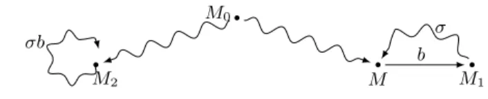
Proof. The proof follows the schema in Figure 3. Assume towards a contradiction that M1< M2is a b-problematic pair. Let M be the marking such that M [biM1
(reachable since M1 is reachable by b). By the assumption, M is a home state,
hence there exists a path σ from M1 to M . Applying σb in M2 (possible by
monotonicity) leads to M2 back, with b as the last transition, hence (M1, M2) is
not b-problematic against the hypothesis. ut
Proposition 4. Let N be a cyclic net and b ∈ T one of its transitions. There
• M0 • M • M1 • M2 b σ σb
Fig. 3. Idea of the proof of Proposition 3.
Proof. Directly from Proposition 3, since in a cyclic net every reachable marking
is a home state. ut
Corollary 3. Each cyclic net is reversible.
The inverse implication does not hold, since one has to actually add effect-reverses to obtain a cyclic net. Moreover, an alternative proof of the result above can be based on the semi-linearity of reachability set for cyclic nets [7].
We present below another class of nets where reversibility is decidable.
Proposition 5. Take a net N . If the set of reachable markings which are not
home states is finite then one can decide whether N is reversible or not. Proof. First, we can construct the set of all markings which are not home states (finite by assumption) as follows. We do not discuss whether finiteness is decid-able or not. By [13] one can verify whether a given marking is a home state. Moreover, every marking reachable from a home state is a home state. Hence, we can find all non home states as follows: explore all states starting from the initial one and stop exploring a branch every time you find a home state.
Consider now the construction in Theorem 1. We will decide whether an arbitrary effect-reverse (triggering in a marking M1) of some transition b changes
the set of reachable markings. This happens only if there exists a marking M2>
M1 which is not b-reachable. We will consider a few cases, distinguished by
whether M2 and M1 are home states or not.
If both of them are home states then consider the net N0obtained by changing the initial marking to any home state. N0 has precisely all home states of N (called a home space [6]), including M1and M2, as reachability set and is cyclic.
By Proposition 4 (M1, M2) is not b-problematic in N0, hence M2 must be
b-reachable. Thus it is b-reachable also in N against the hypothesis, hence this case can never happen.
If M2 is not a home state (M1 may be home state or not), then thanks to
Corollary 2 we can check all the combinations of a marking in min(Eb(N ) +
{eff (b)}) (which is a finite over-approximation of the possible first elements thanks to Lemma 3) with a marking which is not a home state (the corresponding set is finite and can be constructed as discussed at the beginning of the proof). Assume M2 is a home state, but M1 is not. Consider the set of all minimal
home states larger than M1. This is finite from Dickson’s Lemma [14]. We can
construct it using the computed set of reachable markings which are not home states and the coverability set [16] which helps to decide whether there will be
any reachable marking larger than the one considered. This way, we can browse a tree of all markings larger than M1, and cut the branch whenever we find a
home state or the considered marking is not coverable.
Suppose that M2 is not in this set, then there is a home state M3, which
is smaller than M2 but larger than M1. If M3 is b-reachable then (M3, M2) is
a problematic pair, which is impossible, since both of them are home states. Otherwise, (M1, M3) is a problematic pair and the net is not reversible. ut
6
Removing problematic pairs
We know from Proposition 1 that we cannot reverse a net N with problematic pairs. In this section we investigate whether a net N that is not reversible can be made reversible by modifying it but preserving its behaviour. First, we consider adding new places to the net, but preserving its behaviour. Second, we allow to completely change the structure of the net, again preserving its behaviour. The second case is a generalisation of the first one, but, surprisingly, they turn out to work well for the same set of nets.
We need to define what exactly “preserving its behaviour” means. We cannot require the reachability graphs to be the same, as done in previous sections, since the set of places changes. We could require them to be isomorphic, but it is enough to have a homomorphism from the restructured net to the original one. Indeed, this weaker condition is enough to prove our results.
If only new places are added, one may try to simply require transitions to have their usual behaviour on pre-existing places. This approach is safe, i.e. by restricting the attention to old places, no new marking appears, and no new transition between markings becomes enabled. Yet, there is the risk to disable transitions, and, as a consequence, to make unreachable some markings which were previously reachable.
We define below the notion of extension of a net N , which requires (1) that no new behaviours will appear, and (2) that previous behaviours are preserved.
Definition 5 (extension of a net). Let N = (P, T, F, M0) be a net. A net
N0= (P ∪ P0, T, F0, M00) is an extension of N if M00 ↓P= M0 and:
1. F0(p, a) = F (p, a) and F0(a, p) = F (a, p) for each p ∈ P and a ∈ T ;
2. for each reachable marking M in N and each reachable marking M0 in N0 such that M0 ↓P= M and each transition b, b is enabled in M0 iff it is
enabled in M .
Notably, from each extension N0 of a net N there is a homomorphism from RG(N0) to RG(N ), as shown by the following lemma.
Lemma 4. Let N = (P, T, F, M0) be a net and N0 = (P ∪ P0, T, F0, M00) an
Proof. The homomorphism is defined by function ↓P: RG(N0) → RG(N ). The
condition on the initial state is satisfied by construction. Let us consider the other condition.
Let us take two markings M10, M20 in RG(N0) and a transition t such that M10[tiM20. Transition t is enabled in M10 ↓P too, thanks to condition 2 in
Def-inition 5, and M10 ↓P [tiM20 ↓P thanks to condition 1 as desired. By induction
on the length of the shortest path from M00 to M10 we can show that M10 ↓P is
reachable in N , thus M10 ↓P and M20 ↓P are in RG(N ).
Let us now take two markings M1, M2 in RG(N ) and a transition t such
that M1[tiM2. Let M10 be such that M10 ↓P= M1. Transition t is enabled in M1
too, thanks to condition 2 in Definition 5, and M10[tiM20 for some M20 such that
M20 ↓P= M2 thanks to condition 1 as desired. By induction on the length of the
shortest path from M0to M1we can show that M10 is reachable in N0, thus M10
and M20 are in RG(N0). This completes the proof. ut
Checking condition 2 of the definition of extension above is equivalent to solving the problem of state space equality, which is in general undecidable [20]. However, it is decidable in many relevant cases. In particular, complementary nets, based on the idea presented in [30], are a special case of extension of a net. Intuitively, a complementary net has one more place p0 for each bounded place p in the original net, with a number of tokens such that at each time the sum of tokens in p and p0 is equal to the bound of tokens for p.
Definition 6 (complementary net). Let N = (P, T, F, M0) be a net. The
complementary net for N is a net N0= (P ∪P0, T, F0, M00) constructed by adding
a complement place p0 for every bounded place p ∈ P obtaining P0 = {p0 | p ∈ bound (N )}. For all M ∈ [M0i and p ∈ bound (N ), we define cM ∈ NP ∪P
0
, such that cM (p) = M (p) and cM (p0) = (maxM00∈[M0iM00(p))−M (p), setting M00 = cM0.
We also set F0(p0, a) = max(F (a, p) − F (p, a), 0) and F0(a, p0) = max(F (p, a) − F (a, p), 0), for all p0 ∈ P0 and a ∈ T . Furthermore, F0(p, a) = F (p, a) and
F0(a, p) = F (a, p) for all p ∈ P and a ∈ T .
Complementary nets are a special case of extension of nets.
Lemma 5. Let N be a net and N0 the complementary net for N . Then N0 is an extension of N .
Proof. Structural conditions hold by construction, while the complementary places do not change the sets of transitions enabled in reachable markings. ut Another example of extension just adds trap places which only collect tokens. Such a place can be used to compute the number of times a given transition fires. Extending a net N to make it reversible is a very powerful technique. Indeed, we will show below that if there is any reversible net N0 with a homomorphism from RG(N0) to RG(N ), then there is also a reversible extension of N .
Theorem 4. Let N = (P, T, F, M0) be a net. If there is a reversible net N0 =
(P0, T0, F0, M00) and a homomorphism ζ0 from RG(N0) to RG(N ) then there is a reversible extension N00 of N .
Proof. Note that T = T0. Let N00= (P ∪ P0, T, F ∪ F0, M00∪ M0) be the simple
union of N and N0 synchronised on the set of transitions. All the markings in RG(N00) are of the form M0∪ M with ζ0(M0) = M . The proof is a simple
induction on the length of the shorter derivation from M00∪ M0 to M0∪ M .
We show below that N00 is an extension of N . The condition 1 holds by the construction. Let us check condition 2. A transition t enabled in a marking M0∪M of N00is also trivially enabled in marking M of N . Viceversa, a transition
t enabled in marking M of N is also enabled in any marking M0∪ M of N00.
Indeed, since there is a homomorphism from RG(N0) to RG(N ), t is enabled in M0. Being enabled in both M0 and M it is enabled also in M0∪ M .
We now show that RG(N00) and RG(N0) are isomorphic. We define the iso-morphism as ζ00(M0∪ M ) = M0. Existence of corresponding transitions follows
as above. We also note that ζ00 is bijective since M = ζ0(M0), hence RG(N00) and RG(N0) are isomorphic.
We now have to show that N00is reversible. Assume towards a contradiction that it is not, hence from Corollary 1 it has a problematic pair (M10∪ M1, M20∪
M2). M10∪ M1< M20∪ M2 implies M10 < M20, and from the isomorphism M10 is
reachable by b while M20 is not, hence (M10, M20) is problematic in N0, against the hypothesis that M0 is reversible. This concludes the proof. ut The previous result shows that if there is a reversible net with the same behaviour as a given net, then the given net also has a reversible extension.
We can also instantiate the result above in terms of the solvability of the reversed transition system of a given net.
Definition 7 (Reversed transition system). The reversed transition system
of net N is obtained by taking the reachability graph RG(N ) of net N and by adding for each arc (M1, a, M2) in RG(N ) a new arc (M2, a−, M1).
If the reversed transition system is synthesisable, then it can also be solved by an extension of the original net.
Theorem 5. Let N = (P, T, F, M0) be a net and T S its reversed transition
system. If T S is synthesisable, then N has a reversible extension.
Proof. Let N0 = (P0, T0, F0, M00) be a solution of T S. By definition RG(N0) without reverse transitions and RG(N ) are isomorphic. Using the technique in the proof of Theorem 4 we can show that the simple union of N0without reverse transitions and N synchronised on transitions is an extension of N . Furthermore, one can add reverse transitions by synchronising the reverse in N with the re-verse in N0, and this does not change the set of reachable markings. Indeed, an additional marking would be reachable in N0 too, against the hypothesis. ut Hence the questions “Is the reversed transition system of a net N synthesisable?” and “Can we find a reversible extension of a net N ?” are equivalent. From now on we will concentrate on the second formulation.
Thanks to Corollary 1, this second formulation is also equivalent to “Can we find an extension N0 of a net N such that, for each transition b, net N0 has
no b-problematic pair?”. Naturally, the answer to this question depends on the structure of the set of b-problematic pairs in N .
We discuss below the answer to this question in various classes of nets. For instance, we can give a positive answer to the question if for each problematic pair (M1, M2) in N there is at least a bounded place p such that the number
of tokens in p in M1 and in M2 is different. Indeed, such pairs are no more
b-problematic in the complementary net, which is thus reversible.
However, this is not the case for all nets. In particular, there is no reversible extension of the Petri Net in N1 in Figure 1, as shown by the result below.
Example 1. In order to show that there is no reversible extension N0 of the net N1 in Figure 1 we show that any extension of N1has at least one b-problematic
pair. We show, in particular, that the pair of markings ([1, 1], [2, 1]) remains b-problematic in any extension. Assume this is not the case. Then one of the new places, let us call it p, should have less tokens in M2 than in M1. In particular,
this should happen if we go to M1via b and to M2 via bba. Hence, the effect of
ba on p should be negative. This is not possible, since we have an infinite path (ba)∗, which would be disabled against the hypothesis.
As a consequence of Theorem 5, the reversed transition system of N1 is not
synthesisable. We can generalise the example above as follows:
Lemma 6. If a net N has a b-problematic pair (M1, M2) such that M2 is
reach-able from M1 by σ, and there is a marking M ∈ [M0i where σω is enabled then
there is no reversible extension N0 of N .
Unfortunately, the above result together with the construction of comple-mentary nets do not cover the whole spectrum of possible behaviours. We give below two examples of nets that do not satisfy the premises of Lemma 6 and where b-problematic pairs cannot be removed using complementary nets. How-ever, in Example 2 there is an extension where b can be reversed, while this is not the case in Example 3.
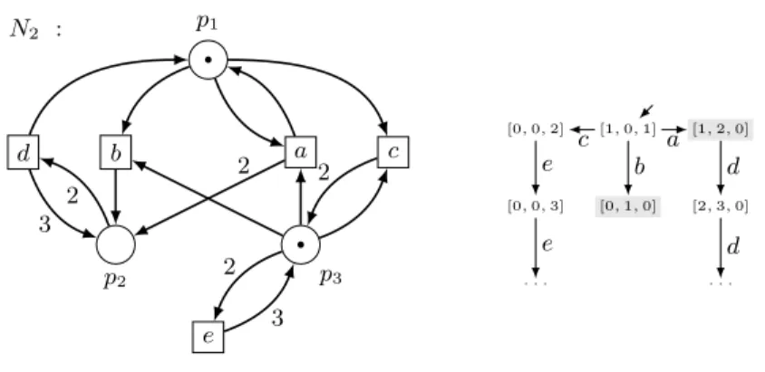
Example 2. Consider the net N2 in Figure 4. There is only one minimal
b-problematic pair, composed of two markings M1 = [0, 1, 0] and M2 = [1, 2, 0]
(emphasised in grey). This pair does not satisfy the premises of Lemma 6. More-over, all places in this net are unbounded and we cannot use the complementary net construction. However, one can consider adding a forth place pb which is
a postplace of transition b (with weight 1). After that, since M1(pb) = 1 and
M2(pb) = 0, the two considered markings no longer form a b-problematic pair.
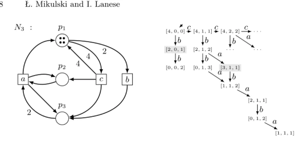
Note that, however, markings [1, 2, 0] and [2, 3, 0] form an a-problematic pair that satisfies the premises of Lemma 6 and hence the whole net cannot be reversed. Example 3. Consider net N3 in Figure 5. All places in N3 are unbounded, and
the computation c(caba)ω is enabled in N
3, hence additional places that count
the number of executions of each transition are unbounded as well. Therefore we cannot use the idea described in Example 2, nor the complementary net.
N2 : p1 p2 p3 a b c d e • • 2 2 3 2 3 2 [1, 0, 1] [0, 1, 0] [1, 2, 0] [2, 3, 0] . . . [0, 0, 2] [0, 0, 3] . . . b a d d c e e
Fig. 4. Net N2 and part of its reachability graph.
We show now that Lemma 6 cannot be used either. Suppose that there is a b-problematic pair (M1, M2) with M2 reachable from M1. This means that the
computation M0[σiMx[biM1[ρiM2 is enabled in N3. Note that for every
reach-able marking M : (i) if M [bci then M [cbi and (ii) if M (p3) > 1 then M [bai implies
M [abi, (iii) if M (p1) > 3 then M [baci implies M [cabi. Moreover if M (p3) ≤ 1
then a is not enabled at M while if M (p1) ≤ 2 then ac is not enabled at M .
Let ρ0bσ0be such that M
x[ρ0iMz[biMy[σ0iM2and σ0is the shortest possible. By
rearrangement (i) described above, σ0 starts with a (otherwise we can move b
forward and σ0is not the shortest possible). In order for a to be enabled we need My(p3) ≥ 2, but if My(p3) > 2 we could swap a and b against the hypothesis
that σ0 is minimal. Hence, the only possibility is My(p3) = 2. Thus aa is not
enabled. Hence, σ0is a or it starts with ac. Let us consider the second case. Since ac is enabled we have My(p1) > 2. By rearrangment (iii) we have Mz(p1) ≤ 3
which implies My(p1) ≤ 1, otherwise σ0 would not be minimal, hence this case
can never happen. Thus, σ0 = a, My(p3) = 2, M2(p3) = 1. As a consequence,
Mx(p3) < M1(p3) ≤ M2(p3) = 1 (as M1 and M2 form a problematic pair) and
the only possibility is Mx(p3) = 0. The only reachable marking with no tokens
in p3is the initial marking [4, 0, 0]. Thus, M1= [2, 0, 1] which is a contradiction,
since the only marking reachable from [2, 0, 1] is b-reachable. Hence, Lemma 6 cannot be used.
Fortunately, we can reuse the reasoning from Example 1. We have to show that the pair of states marked in grey remains b-problematic for every extension of N3. Assume that there exists an extension of N3 for which markings M10
and M20 corresponding to M1 and M2 do not form a b-problematic pair. This
means that there is a new place p such that M10(p) > M20(p). In particular, effp(b) > effp(c) + effp(b) + effp(a). Hence the effect of ca is negative. This is not possible since we have an infinite path c(ca)∗, which would be disabled, against Definition 5. Hence no reversible extension exists.
N3 : p2 p1 p3 a c b •• •• 2 2 4 4 [4, 0, 0] [2, 0, 1] [0, 0, 2] [4, 1, 1] [2, 1, 2] [0, 1, 3] [4, 2, 2] . . . [3, 1, 1] [1, 1, 2] . . . . . . [2, 1, 1] [0, 1, 2] [1, 1, 1] b b c b b c a a b c a b a b a
Fig. 5. Unsolvable net N3 and part of its reachability graph.
7
Conclusions
In the paper we presented an approach to equip a possibly unbounded Petri net with a set of effect-reverses for each transition without changing the set of reachable markings. We have shown that, contrarily to the bounded case, this is not always possible. We introduced the notion of b-problematic pair of markings, which makes the analysis of the net easier.
We have shown, in particular, that a net can be reversed iff it has no b-problematic pairs. Furthermore, we have shown that sometimes b-b-problematic pairs can be removed by extending the net, and that, if the labelled transition system of the reverse net is synthesisable, then this can always be done.
However, our techniques cannot cover the whole class of Petri nets, since the undecidability of the existence of at least one b-problematic pair remains. This result might surprise, since there exist only finitely many minimal b-problematic pairs, and one can easily compute a finite over-approximation of the set contain-ing all the first components of such minimal b-problematic pairs.
The particular case above shows that Dickson’s Lemma guarantees finiteness of a set of minimals, but not the decidability of its emptiness. In order to use Dickson’s Lemma constructively to compute all the elements in this finite set, we need a procedure deciding whether there exists any element larger than a given one. But this is just another formulation of the emptiness problem we want to solve using Dickson’s Lemma constructively. In our opinion, this is the main reason of the counter-intuitiveness of some facts presented in this paper.
As future work one can try to reduce the gap between the sets of nets for which we can and we cannot add effect-reverses. Also, exploiting results of [22] on the undecidability of reachability sets for nets with 5 unbounded places, one may try bound the number of unbounded places needed to prove undecidability of the transition reversibility problem.
Furthermore, the relation between the results above and reversibility in other models should be explored. As already mentioned, reversibility is the notion normally used in process calculi [12], programming languages [33,26] and Turing
machines [5]. The Janus approach [33] obtains reversibility without using history information, as we do in Section 5. This approach requires a carefully crafted language, e.g., assignments, conditional and loops in Janus are nonstandard. Ensuring reversibility in existing models (from Turing machines [5] and CCS [12] to Erlang [26]) normally requires history information, and indeed in Section 6 additional places are used to keep such history information. However, while most of the approaches use dedicated constructs to store history information, here we add history information within the model, and this explains why this is not always possible. This is always possible in Turing machines [5], which are however sequential, while Petri nets are concurrent, and more expressive than Petri nets. The only result in the concurrency literature we are aware of showing that history information can be coded inside the model is the mapping of reversible higher-order pi-calculus into higher-higher-order pi-calculus in [25], which however completely changes the structure of the system, while here we only add new places preserving the original backbone of the system. Indeed, our result is close to [17] where reversibility for distributed Erlang programs is obtained via monitoring, since both approaches feature a distributed state and a minimal interference with the original system. Yet the approach in [17] requires a known and well-behaved communication structure ensured by choreographies. Summarising, the results in this paper can help in answering general questions about reversibility, such as “Which kinds of systems can be reversed without history information?” and “Which kinds of systems can be reversed using only history information modelled inside the original language and preserving the structure of the system?”
References
1. E. Badouel, L. Bernardinello, and P. Darondeau. Petri Net Synthesis. Springer, 2015.
2. K. Barylska, E. Erofeev, M. Koutny, Ł. Mikulski, and M. Piątkowski. Reversing transitions in bounded Petri nets. Fundamenta Informaticae, 157(4):341–357, 2018. 3. K. Barylska, M. Koutny, Ł. Mikulski, and M. Piątkowski. Reversible computation vs. reversibility in Petri nets. Science of Computer Programming, 151:48–60, 2018. 4. K. Barylska and Ł. Mikulski. On decidability of persistence notions. In 24th
Workshop on Concurrency, Specification and Programming, pages 44–56, 2015.
5. C. H. Bennett. Logical reversibility of computation. IBM J. Res. Dev., 17(6):525– 532, 1973.
6. E. Best and J. Esparza. Existence of home states in Petri nets is decidable. Inf.
Process. Lett., 116(6):423–427, 2016.
7. Z. Bouziane and A. Finkel. Cyclic petri net reachability sets are semi-linear effec-tively constructible. In Infinity, ENTCS, pages 15–24. Elsevier, 1997.
8. E. Cardoza, R. Lipton, and A. Meyer. Exponential space complete problems for Petri nets and commutative semigroups (preliminary report). In Proceedings of
STOC’76, pages 50–54. ACM, 1976.
9. C. D. Carothers, K. S. Perumalla, and R. Fujimoto. Efficient optimistic parallel simulations using reverse computation. ACM TOMACS, 9(3):224–253, 1999. 10. M. Colange, S. Baarir, F. Kordon, and Y. Thierry-Mieg. Crocodile: a
symbol-ic/symbolic tool for the analysis of symmetric nets with bag. In ATPN, pages 338–347. Springer, 2011.
11. W. Czerwiński, S. Lasota, R. Lazic, J. Leroux, and F. Mazowiecki. The reachability problem for petri nets is not elementary. arXiv preprint arXiv:1809.07115, 2018. 12. V. Danos and J. Krivine. Reversible communicating systems. In Proceedings of
CONCUR’04, LNCS, pages 292–307. Springer, 2004.
13. D. de Frutos Escrig and C. Johnen. Decidability of home space property. Universit´e de Paris-Sud. Centre d’Orsay. LRI, 1989.
14. L. E. Dickson. Finiteness of the odd perfect and primitive abundant numbers with n distinct prime factors. American Journal of Mathematics, 35(4):413–422, 1913. 15. J. Esparza and M. Nielsen. Decidability issues for Petri nets. BRICS Report Series,
1(8), 1994.
16. A. Finkel. The minimal coverability graph for Petri nets. In ATPN’91, pages 210–243, 1991.
17. A. Francalanza, C. A. Mezzina, and E. Tuosto. Reversible choreographies via monitoring in erlang. In DAIS, LNCS, pages 75–92. Springer, 2018.
18. S. Ginsburg and E. Spanier. Bounded ALGOL-like languages. Transactions of the
American Mathematical Society, 113(2):333–368, 1964.
19. M. Hack. Petri nets and commutative semigroups. Technical Report CSN 18, MIT Lab. for Comp. Sci., Project MAC, 1974.
20. M. Hack. Decidability questions for Petri nets. PhD thesis, MIT, 1976.
21. S. Haddad, F. Kordon, L. Petrucci, J.-F. Pradat-Peyre, and L. Treves. Efficient state-based analysis by introducing bags in Petri nets color domains. In ACC, pages 5018–5025. IEEE, 2009.
22. P. Jancar. Undecidability of bisimilarity for petri nets and some related problems.
Theoretical Computer Science, 148(2):281–301, 1995.
23. D. Kezić, N. Perić, and I. Petrović. An algorithm for deadlock prevention based on iterative siphon control of Petri net. Automatika: ˇcasopis za automatiku, mjerenje, elektroniku, raˇcunarstvo i komunikacije, 47(1-2):19–30, 2006.
24. R. Landauer. Irreversibility and heat generated in the computing process. IBM
Journal of Research and Development, 5:183 –191, 1961.
25. I. Lanese, C. A. Mezzina, A. Schmitt, and J. Stefani. Controlling reversibility in higher-order pi. In CONCUR, LNCS, pages 297–311. Springer, 2011.
26. I. Lanese, N. Nishida, A. Palacios, and G. Vidal. A theory of reversibility for Erlang. J. of Logical and Algebraic Methods in Programming, 100:71–97, 2018. 27. J. S. Laursen, U. P. Schultz, and L. Ellekilde. Automatic error recovery in robot
assembly operations using reverse execution. In IROS, pages 1785–1792. IEEE, 2015.
28. J. Leroux. Vector addition system reversible reachability problem. In CONCUR’11, pages 327–341, 2011.
29. J. McNellis, J. Mola, and K. Sykes. Time travel debugging: Root causing bugs in commercial scale software. CppCon talk, https://www.youtube.com/watch?v= l1YJTg_A914, 2017.
30. T. Murata. Petri nets: Properties, analysis and applications. Proceedings of the
IEEE, 77(4):541–580, 1989.
31. S. A. Reveliotis and J. Y. Choi. Designing reversibility-enforcing supervisors of polynomial complexity for bounded Petri nets through the theory of regions. In
ICATPN’06, pages 322–341, 2006.
32. V. V. Shende, A. K. Prasad, I. L. Markov, and J. P. Hayes. Synthesis of reversible logic circuits. IEEE Trans. on CAD of Integr. Circuits Syst., 22(6):710–722, 2003. 33. T. Yokoyama and R. Gl¨uck. A reversible programming language and its invertible