Fast Approximation Algorithms for Task-Based Runtime Systems

HAL Id: hal-01878606

https://hal.inria.fr/hal-01878606

HAL is a multi-disciplinary open access

archive for the deposit and dissemination of sci-entific research documents, whether they are pub-lished or not. The documents may come from teaching and research institutions in France or abroad, or from public or private research centers.

L’archive ouverte pluridisciplinaire HAL, est destinée au dépôt et à la diffusion de documents scientifiques de niveau recherche, publiés ou non, émanant des établissements d’enseignement et de recherche français ou étrangers, des laboratoires publics ou privés.

Fast Approximation Algorithms for Task-Based Runtime

Systems

Olivier Beaumont, Lionel Eyraud-Dubois, Suraj Kumar

To cite this version:

Olivier Beaumont, Lionel Eyraud-Dubois, Suraj Kumar. Fast Approximation Algorithms for Task-Based Runtime Systems. Concurrency and Computation: Practice and Experience, Wiley, 2018, 30 (17), �10.1002/cpe.4502�. �hal-01878606�

DOI: xxx/xxxx

ARTICLE TYPE

Fast Approximation Algorithms for Task-Based Runtime Systems

Olivier Beaumont

_{| Lionel Eyraud-Dubois*}

_{| Suraj Kumar}

1_{RealOPT, Inria, Bordeaux, France} 2_{University of Bordeaux, France} 3_{Ericsson Research, India}

Correspondence

*Lionel Eyraud-Dubois, Email: Lionel.Eyraud-Dubois@inria.fr

Abstract

In High Performance Computing, heterogeneity is now the norm with specialized accelerators like GPUs providing efficient computational power. Resulting com-plexity led to the development of task-based runtime systems, where complex computations are described as task graphs, and scheduling decisions are made at run-time to perform load balancing between all resources of the platforms. Developing good scheduling strategies, even at the scale of a single node, and analyzing them both theoretically and in practice is expected to have a very high impact on the perfor-mance of current HPC systems. The special case of two kinds of resources, typically CPUs and GPUs is already of great practical interest. The scheduling policy Hetero-Prio has been proposed in the context of fast multipole computations (FMM), and has been extended to general task graphs with very promising results. In this paper, we provide a theoretical study of the performance of HeteroPrio, by proving approx-imation bounds compared to the optimal schedule, both in the case of independent tasks and in the case of general task graphs. Interestingly, our results establish that spoliation (a technique that enables resources to restart uncompleted tasks on another resource) is enough to prove bounded approximation ratios for a list scheduling algorithm on two unrelated resources, which is known to be impossible otherwise. This result holds true both for independent and dependent tasks graphs. Additionally, we provide an experimental evaluation of HeteroPrio on real task graphs from dense linear algebra computation, that establishes its strong performance in practice. KEYWORDS:

List scheduling; Approximation proofs; Runtime systems; Heterogeneous scheduling; Dense linear algebra

1

INTRODUCTION

Accelerators such as GPUs are more and more commonplace in processing nodes due to their massive computational power, usually beside multicores. When trying to exploit both CPUs and GPUs, several phenomena are added to the inherent complexity of the underlying NP-hard optimization problem. First, multicores and GPUs are highly unrelated resources, even in the context of regular linear algebra kernels. Indeed, depending on the kernel, the performance of the GPUs with respect to the one of CPUs may be much higher, close or even worse. In the scheduling literature, unrelated resources are known to make scheduling problems harder (see (1) for a survey on the complexity of scheduling problems, (2) for the specific simpler case of independent tasks scheduling and (3) for a recent survey in the case of CPU and GPU nodes). Second, the variety of existing architectures of processing nodes has increased dramatically with the combination of available resources and the use of both multicores and

BEAUMONT .

accelerators. In this context, developing optimized hand-tuned kernels for all these architectures turns out to be extremely costly. Third, CPUs and GPUs of the same node share many resources (caches, buses,...) and exhibit complex memory access patterns (due to NUMA effects in particular). Therefore, it becomes extremely difficult to predict precisely the durations of both tasks and data transfers, on which traditional offline schedulers rely to allocate tasks, even on very regular kernels such as linear algebra. On the other hand, this situation favors dynamic scheduling strategies where decisions are made at runtime based on the (dynamic) state of the machine and on the (static) knowledge of the application. The state of the machine can be used to allocate a task close to its input data, whereas the knowledge of the application can be used to favor tasks that are close to the critical path. In the recent years, several such task-based runtime systems have been developed, such as StarPU (4), StarSs (5), Super-Matrix (6), QUARK (7), XKaapi (8) or PaRSEC (9). All these runtime systems model the application as a DAG, where nodes correspond to tasks and edges to dependencies between these tasks. These runtime systems are typically designed for linear algebra applications, and the task typically corresponds to a linear algebra kernel whose granularity is well suited for all types of resources. At runtime, the scheduler knows (i) the state of the different resources (ii) the set of tasks that are currently processed by all non-idle resources (iii) the set of ready (independent) tasks whose dependencies have all been solved (iv) the location of all input data of all tasks (v) possibly an estimation of the duration of each task on each resource and of each communication between each pair of resources and (vi) possibly priorities associated to tasks that have been computed offline. Therefore, the runtime system faces the problem of deciding, given an independent set of tasks (and possibly priorities computed by an offline algorithm), given the characteristics of these tasks on the different resources (typically obtained through benchmarking), where to place and to process them.

In the case of independent tasks, on the theoretical side, several solutions have been proposed for this problem, including a PTAS (see for instance (10)). Nevertheless, in the context of runtime systems, the dynamic scheduler must take its decisions at runtime and is itself on the critical path of the application. This reduces the spectrum of possible algorithms to very fast ones, whose complexity to decide which task to process next is typically sublinear in the number of ready tasks.

Several scheduling algorithms have been proposed in this context and can be classified in several classes. The first class of algorithms is based on (variants of) HEFT (11), where the priority of tasks is computed based on their expected distance to the last node, with several possible metrics to define the expected durations of tasks (given that tasks can be processed on heterogeneous resources) and data transfers (given that input data may be located on different resources). To the best of our knowledge there is no approximation ratio for this class of algorithms on unrelated resources, and Bleuse et al. (3) have exhibited an example on 𝑚 CPUs and 1 GPU where HEFT algorithm achieves a makespan Ω(𝑚) times worse the optimal. The second class of scheduling algorithms is based on more sophisticated ideas that aim at minimizing the makespan of the set of ready tasks (see for instance (3, 12)). In this class of algorithms, the main difference lies in the compromise between the quality of the scheduling algorithm (expressed as its approximation ratio when scheduling independent tasks) and its cost (expressed as the complexity of the scheduling algorithm). At last, a third class of algorithms has recently been proposed (see for instance (13, 14, 15, 16)), in which scheduling decisions are based on the affinity between tasks and resources, i.e. try to process the tasks on the best suited resource for it. We will discuss the related work on independent and dependent tasks scheduling in more detail in Section 3.

In this paper, we focus on HETEROPRIO(13, 15, 16)) that belongs to the third class. This algorithm has been proposed in practical settings to benefit as much as possible from platform heterogeneity (17), and has obtained good performance in this context. We are interested in a theoretical analysis of its performance, and we start with the simpler setting of independent tasks. More specifically, we define precisely in Section 2 a variant called HeteroPrioIndep that combines the best of all worlds. Indeed, after introducing notations and general results in Section 4, we first prove that contrarily to HEFT variants, HeteroPrioIndep achieves a bounded approximation ratio in Section 5 while having a low complexity. We also provide a set of proven and tight approximation results, depending on the number of CPUs and GPUs in the node. In Section 6, we analyse HeteroPrioDep, an extension to general task graphs, by applying it at each scheduling stage to the set of independent ready tasks, and we prove that this extended version also achieves a bounded (with respect to the number of resources) approximation ratio. At last, we provide in Section 7 a set of experimental results showing that, besides its very low complexity, HETEROPRIOachieves better performance than the other schedulers based either on HEFT or on approximation algorithms for independent tasks scheduling. Concluding remarks are given in Section 8.

DPOTRF DTRSM DSYRK DGEMM

CPU time / GPU time 1.72 8.72 26.96 28.80

TABLE 1 Acceleration factors for Cholesky kernels (tile size 960).

2

PRESENTATION OF H

P

2.1

Affinity Based Scheduling

HETEROPRIOhas been proposed in the context of task-based runtime systems responsible for allocating tasks onto heterogeneous nodes typically consisting of a few CPUs and GPUs (17).

Historically, most systems use scheduling strategies inspired by the well-known HEFT algorithm: tasks are ordered by prior-ities (which are computed offline) and the highest priority ready task is allocated onto the resource that is expected to complete it first, given the expected transfer times of its input data and the expected processing time of this task on this resource. These systems have shown some limits (13) in strongly heterogeneous and unrelated systems, which is the typical case of nodes con-sisting of both CPUs and GPUs. Indeed, with such nodes, the relative efficiency of accelerators, that we denote as the affinity in what follows, strongly differs from one task to another. Let us for instance consider the case of Cholesky factorization, where 4 types of tasks (kernelsDPOTRF,DTRSM,DSYRKandDGEMM) are involved, on our local platform consisting of 20 CPU cores of two Haswell Intel R Xeon R E5-2680 processors and 4 Nvidia K40-M GPUs. The acceleration factors are depicted in Table 1 .

In the rest of this paper, acceleration factor is always defined as the ratio between the processing times on a CPU and on a GPU, so that the acceleration factor can be smaller than 1 if CPUs turn out to be faster on a given kernel. From this table, we can observe the main characteristics that will influence our model and the design of HETEROPRIO. The acceleration factor strongly depends on the kernel. Some kernels, likeDSYRKandDGEMMare almost 29 times faster on GPUs, whileDPOTRFis only slightly accelerated. This justifies the interest of runtime scheduling policies where the affinity between tasks and resources plays the central role. HETEROPRIObelongs to this class, and its principle is the following: when a resource becomes idle, HETEROPRIO

selects among the ready tasks the one for which it has a maximal affinity. For instance, in the case of Cholesky factorization, among the ready tasks, CPUs will preferDPOTRFtoDTRSMtoDSYRKand toDGEMMwhile GPUs will preferDGEMMtoDSYRK

toDTRSMtoDPOTRF. With this simple definition, HETEROPRIObehaves like a list scheduling algorithm: if some resource is idle and ready tasks exist, HETEROPRIOassigns one of the ready tasks to the idle resource. It is known that list scheduling algorithms are prone to pathological cases with unrelated processors: for a given 𝑋 > 0, consider an instance with one CPU, one GPU, and two tasks. Task 𝑇₁has length 1 + 𝜖 on the CPU and 1∕𝑋 on the GPU, and task 𝑇₂has length 𝑋 on the CPU and 1 on the GPU. Since task 𝑇₁has a better acceleration factor, it is processed on the GPU at time 0, and the idle CPU is forced to process the (very long) task 𝑇₂, leading to a makespan of 𝑋. But scheduling both tasks on the GPU yields a makespan of 1 + 1∕𝑋, and thus an arbitrarily high ratio.

For this reason, we propose to enhance HETEROPRIOwith a spoliation mechanism, defined in the following way. When a fast resource becomes idle and no ready task is available, if it is possible to restart a task already started on another resource and to complete it earlier, then the task is cancelled and restarted on the fast resource. We call this mechanism a spoliation in order to avoid a possible confusion with preemption. Indeed, it does not correspond to preemption since all the progress made on the slow resource is lost. It is therefore less efficient than preemption but it can be implemented in practice, unlike preemption on heterogeneous resources like CPUs and GPUs. This spoliation mechanism can be viewed in two different ways. If it is technically feasible to keep a copy of all data used by tasks running on slow resources, then spoliating tasks running on them is possible and HETEROPRIOin this context is a completely online (non-clairvoyant) algorithm. This mechanism does not exist in StarPU, but it would be feasible at the cost of additionnal memory costs; in larger scale systems (like Hadoop), it is actually used to cope with nodes that have unexpectedly long computation times. Otherwise, we can see HETEROPRIOas a completely offline algorithm: we see spoliation as a way to simplify the presentation of the algorithm, and we use it to compute an offline schedule in which spoliated tasks are actually never started. This schedule is thus completely valid in the standard scheduling model.

This HETEROPRIOallocation strategy has been studied in the context of StarPU for several linear algebra kernels and it has been proven experimentally that it enables to achieve a better utilization of slow resources (13) than other standard HEFT-based strategies.

BEAUMONT .

In the rest of the paper, since task based runtime systems see a set of independent tasks, we will concentrate first on this problem. We present HeteroPrioIndep, a version of HETEROPRIOtargeted at independent tasks, for which we prove approxima-tion ratios under several scenarios for the composiapproxima-tion of the heterogeneous node (namely 1 GPU and 1 CPU, 1 GPU and several CPUs and several GPUs and several CPUs) in Section 5. We extend HETEROPRIOto task graphs and obtain HeteroPrioDep, for which we prove (much weaker) approximation ratios in Section 6.

2.2

H

P

Algorithm for a set of Independent Tasks

Algorithm 1 The HeteroPrioIndep Algorithm for a set of independent tasks

1: Sort Ready Tasks in Queue 𝑄 by non-increasing acceleration factors

2: while there exists an unprocessed task do 3: if all workers are busy then

4: continue 5: end if

6: Select an idle worker 𝑊 7: if 𝑄≠ ∅ then

8: Consider a task 𝑇 from the beginning (resp. the end) of 𝑄 if 𝑊 is a GPU (resp. CPU) worker. 9: Start processing 𝑇 on 𝑊 .

10: else

11: Consider tasks running on the other type of resource in decreasing order of their expected completion time. If the expected completion time of 𝑇 running on a worker 𝑊′_{can be improved on 𝑊 , then 𝑇 is spoliated and 𝑊 starts processing}

𝑇.

12: end if 13: end while

When priorities are associated to tasks, then Line 1 of Algorithm 1 takes them into account for breaking ties among tasks with the same acceleration factor and places the highest priority task first in the scheduling queue. Approximation factors proven in this paper do not depend on how ties are broken and do not depend on task priorities. However, taking task priorities into account is known to improve makespan in practice and we will therefore use priorities in the experiments performed in Section 7.

The queue 𝑄 of ready tasks in Algorithm 1 can be implemented as a heap. Therefore, the time complexity of Algorithm 1 on 𝑚 CPUs and 𝑛 GPUs is(𝑁 log 𝑁), where 𝑁 is the number of ready tasks and the amortized cost of a scheduling decision is therefore of order_{(log 𝑁). We will prove results on the approximation ratio achieved by Algorithm 1 on different platform} configurations for independent tasks in Sections 4 and 5.

2.3

H

P

for Task Graphs

As already mentioned in Section 1, our goal is to extend HeteroPrioIndep designed for independent tasks, to graphs of dependent tasks, and to use HeteroPrioIndep as a building block used by the runtime system to allocate the set of ready tasks. However, in order to obtain guarantees, we need to slightly augment the set of ready tasks. We thus define more precisely HeteroPrioDep: when a GPU (resp. CPU) becomes idle, it picks the task with the highest (resp. lowest) acceleration factor among the ready tasks of 𝑄 or the tasks currently running on the CPU (resp. GPU), provided that it can complete them before their expected completion time. In the latter case, the currently running task is spoliated, i.e. aborted on the CPU (resp. GPU) and restarted on the GPU (resp. CPU).

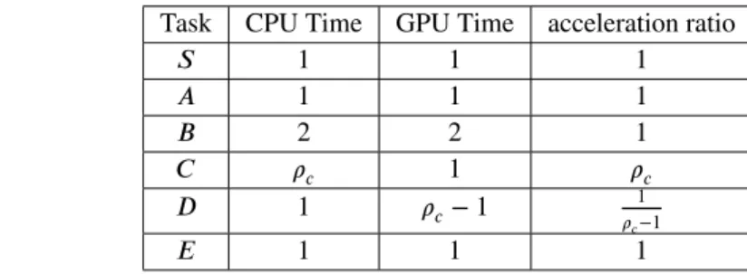
Indeed, such an adaptation of HeteroPrioIndep is necessary to achieve a bounded approximation ratio for task graphs, as shown by the following example. Let us consider a simple platform consisting of 1 CPU and 1 GPU, and the task graph depicted on Figure 1 , together with the expected time of the different tasks on both resource types.

S A C B D E

Task CPU Time GPU Time acceleration ratio

𝑆 1 1 1 𝐴 1 1 1 𝐵 2 2 1 𝐶 𝜌_𝑐 1 𝜌_𝑐 𝐷 1 𝜌_𝑐− 1 1 𝜌𝑐−1 𝐸 1 1 1

FIGURE 1 A task graph and duration of different tasks.

Let us analyze the behavior on this task graph with an algorithm for which spoliation is forbidden while there exists a ready task. Since tasks 𝑆, 𝐴, 𝐵 and 𝐶 have the same acceleration factor, let us assume1_{that 𝑆 and 𝐴 are processed on the CPU (that}

becomes available at time 2) and task 𝐵 by the GPU (that becomes available at time 3). At time 2, 𝐶 becomes ready and the CPU is available, so that it processes 𝐶 until time 2 + 𝜌_𝑐. Then at time 3, the GPU becomes ready and 𝐷 is the only ready task at that time. If the GPU only considers the set of ready tasks, and not the tasks running on the other resource, it misses the opportunity to process 𝐶 for which it is very well suited since 𝜌 ≫ 1, and processes 𝐷, for which it is badly suited, until time 2 + 𝜌_𝑐. Then both resources are available at time 2 + 𝜌_𝑐 and one picks task 𝐸, so that the makespan is 3 + 𝜌_𝑐if spoliation is forbidden while there exists a ready task.

Moreover, the minimum length of path 𝑆 → 𝐵 → 𝐷 → 𝐸 is 5, so that 𝐶_maxO𝑝𝑡 ≥ 5. Similarly, if 𝑆, 𝐵, 𝐶, 𝐸 are scheduled on the GPU and 𝐴, 𝐷 on the CPU, then the completion time is 5, so that 𝐶_maxO𝑝𝑡 = 5, and the approximation ratio achieved when spoliation is forbidden while there exists a ready task would be 𝜌𝑐+3

5 , which can be made arbitrarily large with 𝜌𝑐large enough.

On the other hand, let us consider HeteroPrioDep (Algorithm 2) where spoliation is allowed even if there exists a ready task. Then, at time 3, the best acceleration ratio among the ready tasks (task 𝐷) is 1

𝜌𝑐−𝜖

≪ 1, the best acceleration ratio among the tasks running on the CPU (i.e. task 𝐶) is 𝜌_𝑐 ≫1 and the GPU is able to complete 𝐶 at time 3 + 1 ≪ 2 + 𝜌𝑐, so that 𝐶 is spoliated

and processed on the GPU. In this case, the makespan of HeteroPrioDep is 𝐶_maxO𝑝𝑡 = 5, so that it is optimal on this instance. We will prove general approximation ratios for HeteroPrioDep in Section 6 and evaluate its performance in Section 7.

It is worth noting that spoliating while there exist ready tasks is never useful in the case of independent tasks: indeed, since all tasks are available from the beginning, the situation where both types of resources process tasks for which they are badly suited cannot happen. This is why in the case of independent tasks, we consider the version HeteroPrioIndep, as depicted in Algorithm 1.

3

RELATED WORKS

3.1

Independent Tasks Scheduling

The problem considered in this paper is a special case of the standard unrelated scheduling problem 𝑅||𝐶_max. This problem is made easier by preemption, i.e. the ability of stopping a task and storing its current state on a given machine and then to restart it from its current state onto another machine. In this context, Lawler et al. (18) have proved that the problem can be solved in polynomial time using linear programming. Unfortunately, in particular in the context of CPUs and GPUs, preemption is not feasible in practice. This is why we concentrate in this paper on spoliation, where a task is stopped and restarted from the beginning onto another resource. Without preemption, Lenstra et al (2) proposed a PTAS for the general problem with a fixed number of machines, and propose a 2-approximation algorithm, based on the rounding of the optimal solution of the linear program which describes the preemptive version of the problem. This result has recently been improved (19) to a 2 − 1

𝑚

approximation. However, the time complexity of these general algorithms is too high to allow using them in the context of runtime systems.

The more specialized case with a small number of types of resources has been studied in (10) and a PTAS has been proposed, which also contains a rounding phase whose complexity makes it impractical, even for 2 different types of resources. Greedy

1_{Strictly speaking, this depends on how ties are broken ; however this behavior can be forced by changing the acceleration ratios by arbitrarily small values. We do}

BEAUMONT .

Algorithm 2 The HeteroPrioDep Algorithm for a set of dependent tasks.

1: Sort input tasks in Queue 𝑄 by non-increasing acceleration factors

2: Create an empty Queue of running tasks 𝑄′by non-increasing acceleration factors

3: while there exists an unprocessed task do 4: if all workers are busy then

5: continue 6: end if

7: Select an idle worker 𝑊 8: if 𝑄′≠ ∅ then

9: Consider tasks from the beginning (resp. the end) of 𝑄′if 𝑊 is a GPU (resp. CPU) worker 10: Until finding a candidate task 𝐶′whose completion time would be smaller if restarted on 𝑊 .

11: end if 12: if 𝑄≠ ∅ then

13: Consider a candidate task 𝐶 from the beginning (resp. the end) of 𝑄 if 𝑊 is a GPU (resp. CPU) worker. 14: end if

15: Among 𝐶 and 𝐶′, choose the task 𝑇 with the highest acceleration factor if 𝑊 is a GPU (resp. the smallest acceleration

factor if 𝑊 is a CPU)

16: if a worker 𝑊′of the other type is idle then

17: Process task 𝑇 on its favorite resource between 𝑊 and 𝑊′

18: else

19: Process task 𝑇 on 𝑊 (potentially using spoliation).

20: end if

21: Update 𝑄 and 𝑄′.

22: end while

approximation algorithms for the online case have been proposed by Imreh on two different types of resources (20) and by Chen et al. in (21). In (21), a 3.85-approximation algorithm (CYZ₅) is provided in the case of online scheduling on two types of resources. These algorithms have linear complexity, however most of their decisions are based on comparing task processing times on both types of resources and not on trying to balance the load. Since these algorithms are tailored towards worst-case behavior, their average performance on practical instances is not satisfying (in practice all tasks are scheduled on the GPUs, see Section 7). For example, it is possible to show that there exist instances with arbitrarily small tasks for which the ratio to the optimal solution is bounded by 1.5, whereas the approximation ratio of all other algorithms tends to 1 when the size of tasks tends to 0.

Additionally, Bleuse et al (3, 22) have proposed algorithms with varying approximation factors (4

3, 3

2and 2) based on dynamic

programming and dual approximation techniques. These algorithms have better approximation ratios than the ones proved in this paper, but their time complexity is much higher, as we will discuss in Section 7. Furthermore, we also show in Section 7 that their actual performance is not as good when used iteratively on the set of ready tasks in the context of task graph scheduling. We also exhibit that HETEROPRIOperforms better on average than the above mentioned algorithms, despite its higher worst case approximation ratio.

Finally, there has recently been a number of papers targeting both a low computing cost and a bounded approximation ratio, such as (14, 12, 15). In (14), Cherière et al. propose a 2 approximation algorithm under the assumption that no task is longer on any resource than the optimal makespan. It is worth noting that under this restrictive assumption, Lemma 3 establishes the same approximation ratio for HeteroPrioIndep. The algorithm CLB2C proposed in (14) is based on the same underlying ideas as HETEROPRIO, as tasks are ordered by non-increasing acceleration factors and the highest accelerated task and the less accelerated task compete for being allocated respectively to the least loaded GPU and the least loaded CPU, under a strategy that slightly differs from HeteroPrioIndep. In (15), a preliminary version of this paper is proposed, that concentrate on independent tasks only. In (12), Canon et al. propose two strategies that also achieve a 2 approximation ratio for independent task scheduling. All these results are summarized in Table 2 . We describe these algorithms in detail in Section 7, where we also provide a detailed comparison both in terms of running time and in terms of average approximation ratio on realistic instances. Another

Name Complexity Approximation ratio

CYZ₅(21) 𝑁log(𝑚 + 𝑛) 3.85

LG (20) 𝑁log(𝑚 + 𝑛) 2 +𝑚−1_𝑛

MG(1,1) (20) 𝑁log(𝑚 + 𝑛) 4 − _𝑚2

DualHP (22) 𝑁log(𝑁𝑚𝑛) log(Δ) 2

DualDynamic (22) 𝑁2𝑚2𝑘3log(Δ) 4

3+ 1 3𝑘

DualAccel (22) 𝑁 𝑚log(𝑁) log(Δ) 3

2*

CLB2C (14) 𝑁log(𝑁𝑚𝑛) 2**

BalancedEstimate (12) 𝑁log(𝑁𝑚𝑛) 2

BalancedMakespan (12) 𝑁2log(𝑁𝑚𝑛) 2

HeteroPrioIndep 𝑁log(𝑁) + (𝑁 + 𝑚 + 𝑛) log(𝑚 + 𝑛) 3.42

TABLE 2 Summary of complexity and approximation ratios of different algorithms from the literature. We consider instances

with 𝑁 tasks, and two sets of resources of sizes 𝑛 and 𝑚, with 𝑛 ≤ 𝑚. The parameter Δ is the range of possible makespan values tested by the dual approximation algorithms, and is bounded by∑_𝑖max(𝑝𝑖, 𝑞𝑖) − max𝑖min(𝑝𝑖, 𝑞𝑖). Remarks: * DualAccel

assumes that all tasks execute faster on the GPUs. ** CLB2C assumes that ∀𝑖, max(𝑝𝑖, 𝑞𝑖)≤ 𝐶

O𝑝𝑡 max.

similar experimental comparison is available in (12), but it is limited to the case of independent tasks and based on less realistic randomly-generated instances.

3.2

Task Graph Scheduling

The literature on approximation algorithms for task graph scheduling on heterogeneous machines is more limited. In the case of related resources, Chudak et al. (23) and Chekuri et al. (24) propose a log 𝑚 approximation algorithm, where 𝑚 denotes the number of machines. To the best of our knowledge, these results are still the best approximation algorithms for the case of related machines, even though better approximation ratios are known for special cases, such as chains (25).

The special case of platforms consisting of two kinds of unrelated resources, typically CPUs and GPUs, has recently received a lot of attention. In (26), Kedad-Sidhoum et al. establish the first constant approximation ratio (i.e. 6) in this context. The same approximation ratio (but a better behavior in practice) has also been established in (27). These algorithms are based on a two phases approach, where the assignment of tasks onto resource types is computed using the rounding of the solution of a linear program and then the schedule is computed using a list scheduling approach. We will compare in detail the results obtained by this algorithm in comparison to all variants of HETEROPRIOboth in terms of running time and in terms of average approximation ratio on realistic instances in Section 7.

4

NOTATIONS AND FIRST RESULTS

4.1

General Notations

In this paper, we prove approximation ratios achieved by both HeteroPrioIndep for independent tasks and HeteroPrioDep for task graphs scheduling. The input of the scheduling problem we consider is thus a platform of 𝑛 GPUs and 𝑚 CPUs, a set of independent tasks (or a task graph 𝐺), where task 𝑇_𝑖has processing time 𝑝_𝑖on CPU and 𝑞_𝑖on GPU. Then, the goal is to allocate and schedule those tasks (or a task graph) onto the resources so as to minimize the makespan. We define the acceleration factor of task 𝑇_𝑖as 𝜌_𝑖 = 𝑝𝑖

𝑞𝑖

. 𝐶_maxO𝑝𝑡() and 𝐶maxO𝑝𝑡(𝐺) denote respectively the optimal makespan of set and task graph 𝐺. Throughout

this paper, even in the case of task graph scheduling, we neglect the communication times that happen when data has to be exchanged from CPU to GPU. Indeed, taking them into account would make this hard problem even more complex, and in many practical cases they can be overlapped by the computational tasks. A more precise model which handles communications is left for future work.

BEAUMONT .

4.2

H

P

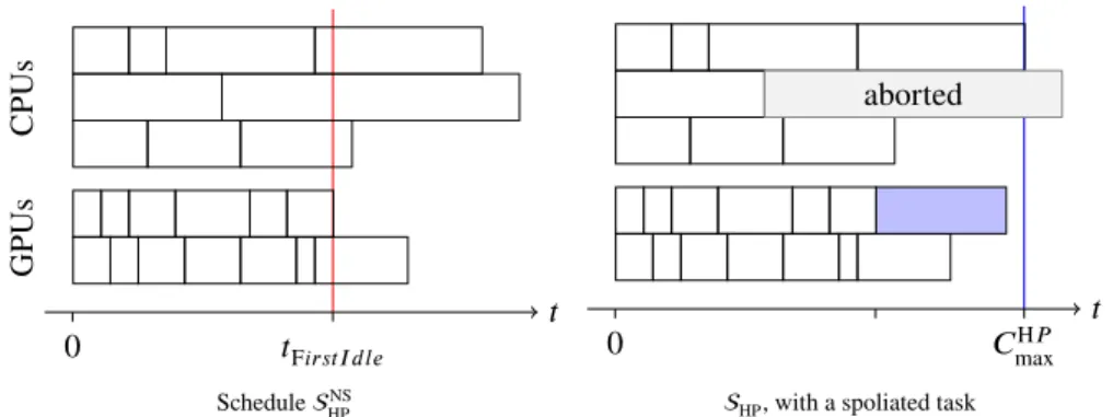
Schedule For a Set of Independent Tasks

To analyze the behavior of HeteroPrioIndep, it is useful to consider the list schedule obtained before any spoliation attempt. We will denote this scheduleNS

HP, and the final HeteroPrioIndep schedule is denotedHP. Figure 2 showsHPNSandHPfor a

set of independent tasks. We define 𝑡F𝑖𝑟𝑠𝑡𝐼 𝑑𝑙𝑒as the first moment any worker is idle inHPNS, which is also the first time any

spoliation can occur. Therefore, after time 𝑡F𝑖𝑟𝑠𝑡𝐼 𝑑𝑙𝑒, each worker processes at most one task inHPNS. Finally, we define 𝐶 H𝑃 max()

as the makespan ofHPon instance.

0 𝑡F𝑖𝑟𝑠𝑡𝐼 𝑑𝑙𝑒 𝑡 CPUs GPUs ScheduleNS HP aborted 0 𝐶H𝑃 max 𝑡

HP, with a spoliated task

FIGURE 2 Example of a HeteroPrioIndep schedule.

4.3

Area Bound For a Set of Independent Tasks

Let us now present and characterize a lower bound on the optimal makespan. This lower bound is obtained by assuming that tasks are fully divisible, i.e. can be processed in parallel on any number of resources without any efficiency loss. More specifically, any fraction 𝑥_𝑖of task 𝑇_𝑖is allowed to be processed on CPUs, and this fraction overall consumes CPU resources for 𝑥_𝑖𝑝_𝑖time units. Then, the lower bound 𝐴𝑟𝑒𝑎𝐵𝑜𝑢𝑛𝑑() for a set of tasks  on 𝑚 CPUs and 𝑛 GPUs is the solution (in rational numbers) of the following linear program.

Minimize 𝐴𝑟𝑒𝑎𝐵𝑜𝑢𝑛𝑑() such that ∑ 𝑖∈𝐼 𝑥_𝑖𝑝_𝑖≤ 𝑚 ⋅ 𝐴𝑟𝑒𝑎𝐵𝑜𝑢𝑛𝑑() (1) ∑ 𝑖∈𝐼 (1 − 𝑥𝑖)𝑞𝑖≤ 𝑛 ⋅ 𝐴𝑟𝑒𝑎𝐵𝑜𝑢𝑛𝑑() (2) 0≤ 𝑥𝑖≤ 1

Since any valid solution to the scheduling problem can be converted into a solution of this linear program, it is clear that

𝐴𝑟𝑒𝑎𝐵𝑜𝑢𝑛𝑑() ≤ 𝐶maxO𝑝𝑡(). Another immediate bound on the optimal is ∀𝑇 ∈ , min(𝑝𝑇, 𝑞𝑇)≤ 𝐶

O𝑝𝑡

max(). By contradiction and

with simple exchange arguments, one can prove the following two lemmas.

Lemma 1. In the area bound solution, the completion time on each type of resources is the same, i.e. constraints (1) and

(2) are both equalities.

Proof. Let us assume that one of the inequality constraints in the area solution is not tight. Without loss of generality, let us assume that Constraint (1) is not tight. Then some load from the GPUs can be transferred to the CPUs, what in turn

decreases the value of 𝐴𝑟𝑒𝑎𝐵𝑜𝑢𝑛𝑑(), in contradiction with the optimality of the solution.

Lemma 2. In 𝐴𝑟𝑒𝑎𝐵𝑜𝑢𝑛𝑑(), the assignment of tasks is based on the acceleration factor, i.e. ∃𝑘 > 0 such that ∀𝑖, 𝑥𝑖 <

Proof. Let us assume∃(𝑇₁,𝑇₂) such that (i) 𝑇₁is partially processed on GPUs (i.e., 𝑥₁ < 1), (ii) 𝑇₂is partially processed

on CPUs (i.e., 𝑥₂>0) and (iii) 𝜌₁< 𝜌₂.

Let 𝑊 𝐶 and 𝑊 𝐺 denote respectively the overall work on CPUs and GPUs in 𝐴𝑟𝑒𝑎𝐵𝑜𝑢𝑛𝑑(). If we transfer a fraction 0 < 𝜖₂ < 𝑚𝑖𝑛(𝑥₂,(1−𝑥1)𝑝1

𝑝2

) of 𝑇₂work from CPU to GPU and a fraction 𝜖2𝑞2

𝑞1

< 𝜖₁ < 𝜖2𝑝2

𝑝1

of 𝑇₁work from GPU to CPU, the

overall loads 𝑊 𝐶′and 𝑊 𝐺′become

𝑊 𝐶′= 𝑊 𝐶 + 𝜖₁𝑝₁− 𝜖₂𝑝₂ 𝑊 𝐺′= 𝑊 𝐺 − 𝜖₁𝑞₁+ 𝜖₂𝑞₂ Since 𝑝1 𝑝₂ < 𝜖₂ 𝜖₁ < 𝑞₁ 𝑞₂, then both 𝑊 𝐶

′ _{< 𝑊 𝐶and 𝑊 𝐺}′ _{< 𝑊 𝐺hold true, and hence the 𝐴𝑟𝑒𝑎𝐵𝑜𝑢𝑛𝑑() is not optimal.}

Therefore,∃ a positive constant 𝑘 such that ∀𝑖 on GPU, 𝜌𝑖≥ 𝑘 and ∀𝑖 on CPU, 𝜌𝑖≤ 𝑘.

This area bound can be extended to the case of non-independent tasks (13, 26) by adding a variable 𝑠_𝑖representing the start time of each task 𝑖, and the following set of constraints:

∀𝑖, 𝑗 such that 𝑖 → 𝑗, 𝑠_𝑖+ 𝑥_𝑖𝑝_𝑖+ (1 − 𝑥_𝑖)𝑞_𝑖≤ 𝑠𝑗 (3)

∀𝑖, 𝑠_𝑖+ 𝑥_𝑖𝑝_𝑖+ (1 − 𝑥_𝑖)𝑞_𝑖≤ 𝐴𝑟𝑒𝑎𝐵𝑜𝑢𝑛𝑑() (4) Constraint (3) ensures that the starting times of all tasks are consistent with their dependencies (𝑥_𝑖𝑝_𝑖+ (1 − 𝑥𝑖)𝑞𝑖 represent

the processing time of task 𝑖), and constraint (4) conveys the fact that the makespan is not smaller than the completion time of all tasks. This mixed bound (which takes into account both area and dependencies) will not be used in our proofs, but is used in Section 7 to analyze the quality of the schedules obtained by all algorithms.

4.4

Summary of Approximation Results

This paper presents several approximation results for HeteroPrioIndep depending on the number of CPUs and GPUs. The following table presents a quick overview of the main results for a set of independent tasks proven in Section 5.

(#CPUs, #GPUs) Approximation ratio Worst case ex.

(1,1) 1+ √ 5 2 1+√5 2 (m,1) 3+ √ 5 2 3+√5 2 (m,n) 2 +√2 ≈ 3.41 2 +√2 3 ≈ 3.15

We also present (𝑚 + 𝑛)-approx proof for HeteroPrioDep on 𝑚 CPUs and 𝑛 GPUs, and a tight worst-case example on 1 CPU and 1 GPU in Section 6.

5

PROOF OF HeteroPrioIndep APPROXIMATION RESULTS

5.1

General Lemmas

The following lemma gives a characterization of the work performed by HeteroPrioIndep at the beginning of the processing, and shows that HeteroPrioIndep performs as much work as possible when all resources are busy. For any time instant 𝑡, let us define′_{(𝑡) as the sub-instance of obtained by removing the fractions of tasks that have been processed between time 0 and}

time 𝑡 by HeteroPrioIndep. Then, a schedule beginning like HeteroPrioIndep (until time 𝑡) and ending like 𝐴𝑟𝑒𝑎𝐵𝑜𝑢𝑛𝑑(′_(𝑡))

completes in 𝐴𝑟𝑒𝑎𝐵𝑜𝑢𝑛𝑑().

Lemma 3. At any time 𝑡≤ 𝑡F𝑖𝑟𝑠𝑡𝐼 𝑑𝑙𝑒inHPNS,

𝑡+ 𝐴𝑟𝑒𝑎𝐵𝑜𝑢𝑛𝑑(′_{(𝑡)) = 𝐴𝑟𝑒𝑎𝐵𝑜𝑢𝑛𝑑()}

Proof. HeteroPrioIndep assigns tasks based on their acceleration factors. Therefore, at instant 𝑡,∃𝑘₁ ≤ 𝑘2 such that (i)

all tasks (at least partially) processed on GPUs have an acceleration factor larger than 𝑘₂, (ii) all tasks (at least partially)

allocated on CPUs have an acceleration factor smaller than 𝑘₁ and (iii) all tasks not assigned yet have an acceleration

BEAUMONT .

After 𝑡, 𝐴𝑟𝑒𝑎𝐵𝑜𝑢𝑛𝑑(′_{) satisfies Lemma 2, and thus ∃𝑘 with 𝑘}

1≤ 𝑘 ≤ 𝑘2such that all tasks of′with acceleration factor

larger than 𝑘 are allocated on GPUs and all tasks of_′_{with acceleration factor smaller than 𝑘 are allocated on CPUs.}

Therefore, combining above results before and after 𝑡, the assignment beginning like HeteroPrioIndep (until time 𝑡)

and ending like 𝐴𝑟𝑒𝑎𝐵𝑜𝑢𝑛𝑑(′_{(𝑡)) satisfies the following property: ∃𝑘 > 0 such that all tasks of with acceleration factor}

larger than 𝑘 are allocated on GPUs and all tasks of with acceleration factor smaller than 𝑘 are allocated on CPUs. This

assignment_{, whose completion time on both CPUs and GPUs (according to Lemma 1) is 𝑡+𝐴𝑟𝑒𝑎𝐵𝑜𝑢𝑛𝑑(}′_{) clearly defines}

a solution of the fractional linear program defining the area bound solution, so that 𝑡+ 𝐴𝑟𝑒𝑎𝐵𝑜𝑢𝑛𝑑(′_{)≥ 𝐴𝑟𝑒𝑎𝐵𝑜𝑢𝑛𝑑().}

Similarly, 𝐴𝑟𝑒𝑎𝐵𝑜𝑢𝑛𝑑() satisfies both Lemma 2 with some value 𝑘′_{and Lemma 1 so that in 𝐴𝑟𝑒𝑎𝐵𝑜𝑢𝑛𝑑(), both CPUs}

and GPUs complete their work simultaneously. If 𝑘′< 𝑘, more work is assigned to GPUs in 𝐴𝑟𝑒𝑎𝐵𝑜𝑢𝑛𝑑() than in , so

that, by considering the completion time on GPUs, we get 𝐴𝑟𝑒𝑎𝐵𝑜𝑢𝑛𝑑() ≥ 𝑡 + 𝐴𝑟𝑒𝑎𝐵𝑜𝑢𝑛𝑑(′_{). Similarly, if 𝑘}′ _{> 𝑘, by}

considering the completion time on CPUs, we get 𝐴𝑟𝑒𝑎𝐵𝑜𝑢𝑛𝑑() ≥ 𝑡 + 𝐴𝑟𝑒𝑎𝐵𝑜𝑢𝑛𝑑(′_).

Since 𝐴𝑟𝑒𝑎𝐵𝑜𝑢𝑛𝑑(_{) is a lower bound on 𝐶max}O𝑝𝑡(), the above lemma implies that 1. at any time 𝑡≤ 𝑡F𝑖𝑟𝑠𝑡𝐼 𝑑𝑙𝑒in

NS

HP, 𝑡 + 𝐴𝑟𝑒𝑎𝐵𝑜𝑢𝑛𝑑(

′_{(𝑡))≤ 𝐶}O𝑝𝑡 max(),

2. 𝑡_{F𝑖𝑟𝑠𝑡𝐼 𝑑𝑙𝑒}≤ 𝐶maxO𝑝𝑡(), and thus all tasks start before 𝐶 O𝑝𝑡

max() in HPNS,

3. if ∀𝑖 ∈_{, max(𝑝𝑖}, 𝑞𝑖)≤ 𝐶

O𝑝𝑡

max(), then 𝐶maxH𝑃() ≤ 2𝐶 O𝑝𝑡 max().

Another interesting characteristic of HeteroPrioIndep is that spoliation can only take place from one type of resource to the other. Indeed, since assignment in_NS

HP is based on the acceleration factors of the tasks, and since a task can only be spoliated if

it can be processed faster on the other resource type, we get the following lemmas.

Lemma 4. If, in_NS

HP, a resource type processes a task whose processing time is not larger on the other resource type, then

no task is spoliated from the other resource type.

Proof. Without loss of generality let us assume that there exists a task 𝑇 processed on a CPU inNS

HP, such that 𝑝𝑇 ≥ 𝑞𝑇. We

prove that in this case, there is no spoliated task on CPUs, which is the same thing as there being no aborted task on GPUs.

𝑇 is processed on a CPU inNS

HP, and

𝑝𝑇

𝑞𝑇 ≥ 1, therefore by definition of HeteroPrioIndep, all tasks on GPUs in 

NS

HPhave

an acceleration factor at least 𝑝𝑇 ′

𝑞𝑇 ′ ≥ 1. Non spoliated tasks running on GPUs after 𝑡F𝑖𝑟𝑠𝑡𝐼 𝑑𝑙𝑒

are candidates to be spoliated by the CPUs. But for each of these tasks, the processing time on CPU is at least as large as the processing time on GPU. It is thus not possible for an idle CPU to spoliate any task running on GPUs, because this task would not complete earlier on the CPU.

Lemma 5. In HeteroPrioIndep, if a resource type executes a spoliated task then no task is spoliated from this resource type.

Proof. Without loss of generality let us assume that 𝑇 is a spoliated task processed on a CPU. From the HeteroPrioIndep

definition, 𝑝_𝑇 < 𝑞_𝑇. It also indicates that 𝑇 was processed on a GPU inNS

HPwith 𝑞𝑇 ≥ 𝑝𝑇. By Lemma 4, CPUs do not have

any aborted task due to spoliation.

Finally, we will also rely on the following lemma, that provides the worst case performance of a list schedule when all tasks lengths are large (i.e. > 𝐶_maxO𝑝𝑡) on one type of resource.

Lemma 6. Let_{ ⊆  such that the processing time of each task of  on one resource type is larger than 𝐶max}O𝑝𝑡(), then any

list schedule of on 𝑘 ≥ 1 resources of the other type has length at most (2 − 1_𝑘)𝐶maxO𝑝𝑡().

Proof. Without loss of generality, let us assume that the processing time of each task of set_{ on CPU is larger than 𝐶max}O𝑝𝑡().

All these tasks must therefore be processed on the GPUs in an optimal solution. If scheduling this set on 𝑘 GPUs can be

done in time 𝐶, then 𝐶_{≤ 𝐶max}O𝑝𝑡(). The standard list scheduling result from Graham (28) implies that the length of any list

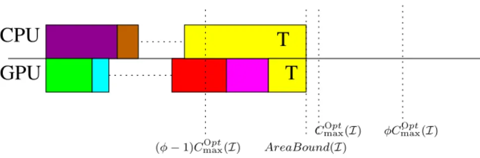
CPU

GPU

T

AreaBound(I)

CmaxOpt(I) φCmaxOpt(I) (φ− 1)CmaxOpt(I)

FIGURE 3 Situation where 𝑇 ends on CPU after 𝜙𝐶_maxO𝑝𝑡().

5.2

Approximation Ratio with 1 GPU and 1 CPU

With the above lemmas, we are able to prove an approximation ratio of 𝜙 = 1+

√ 5

2 for HeteroPrioIndep when the node is

composed of 1 CPU and 1 GPU. We will also prove that this result is the best achievable by providing a task set for which the approximation ratio of HeteroPrioIndep is 𝜙.

Theorem 7. For any instance_{ with 1 CPU and 1 GPU, 𝐶}H𝑃

max() ≤ 𝜙𝐶 O𝑝𝑡 max().

Proof. Without loss of generality, let us assume that the first idle time (at instant 𝑡_{F𝑖𝑟𝑠𝑡𝐼 𝑑𝑙𝑒}) occurs on the GPU and the CPU

is processing the last remaining task 𝑇 . We will consider two main cases, depending on the relative values of 𝑡F𝑖𝑟𝑠𝑡𝐼 𝑑𝑙𝑒and

(𝜙 − 1)𝐶maxO𝑝𝑡.

The easy case is 𝑡F𝑖𝑟𝑠𝑡𝐼 𝑑𝑙𝑒 ≤ (𝜙 − 1)𝐶

O𝑝𝑡

max. Indeed, inHPNS, the completion time of task 𝑇 is at most 𝑡F𝑖𝑟𝑠𝑡𝐼 𝑑𝑙𝑒+ 𝑝𝑇. If

task 𝑇 is spoliated by the GPU, its execution time is 𝑡_{F𝑖𝑟𝑠𝑡𝐼 𝑑𝑙𝑒}+ 𝑞𝑇. In both cases, the completion time of task 𝑇 is at most

𝑡F𝑖𝑟𝑠𝑡𝐼 𝑑𝑙𝑒+ min(𝑝𝑇, 𝑞𝑇)≤ (𝜙 − 1)𝐶 O𝑝𝑡 max+ 𝐶 O𝑝𝑡 max= 𝜙𝐶 O𝑝𝑡 max.

On the other hand, we assume now that 𝑡_{F𝑖𝑟𝑠𝑡𝐼 𝑑𝑙𝑒} > (𝜙 − 1)𝐶maxO𝑝𝑡. If 𝑇 ends before 𝜙𝐶

O𝑝𝑡

max on the CPU inHPNS, since

spoliation can only improve the completion time, this ends the proof of the theorem. In what follows, we assume that the

completion time of 𝑇 on the CPU inNS

HPis larger than 𝜙𝐶

O𝑝𝑡

max(), as depicted in Figure 3 .

It is clear that 𝑇 is the only unprocessed task after 𝐶_maxO𝑝𝑡. Let us denote by 𝛼 the fraction of 𝑇 processed after 𝐶_maxO𝑝𝑡on the

CPU. Then 𝛼𝑝_𝑇 >(𝜙−1)𝐶_maxO𝑝𝑡since 𝑇 ends after 𝜙𝐶_maxO𝑝𝑡by assumption. Lemma 3 applied at instant 𝑡= 𝑡_{F𝑖𝑟𝑠𝑡𝐼 𝑑𝑙𝑒}implies that

the GPU is able to process the fraction 𝛼 of 𝑇 by 𝐶_maxO𝑝𝑡(see Figure 4 ) while starting this fraction at 𝑡_{F𝑖𝑟𝑠𝑡𝐼 𝑑𝑙𝑒≥ (𝜙 − 1)𝐶max}O𝑝𝑡

so that 𝛼𝑞_𝑇 ≤ (1 − (𝜙 − 1))𝐶maxO𝑝𝑡 = (2 − 𝜙)𝐶

O𝑝𝑡

max. Therefore, the acceleration factor of 𝑇 is at least

𝜙−1

2−𝜙 = 𝜙. Since

HeteroPrioIndep assigns tasks on the GPU based on their acceleration factors, all tasks in_{ assigned to the GPU also}

have an acceleration factor at least 𝜙.

Let us now prove that the GPU is able to process_⋃{𝑇 } in time 𝜙𝐶_maxO𝑝𝑡. Let us split_⋃{𝑇 } into two sets1and2

depending on whether the tasks of⋃{𝑇 } are processed on the GPU (1) or on the CPU (2) in the optimal solution. By

construction, the processing time of_1on the GPU is at most 𝐶_maxO𝑝𝑡and the processing of_2on the CPU takes at most 𝐶_maxO𝑝𝑡.

Since the acceleration factor of tasks of2is larger than 𝜙, the processing time of tasks of2on the GPU is at most 𝐶

O𝑝𝑡 max∕𝜙

and the overall processing of_⋃{𝑇 } takes at most 𝐶_maxO𝑝𝑡+ 𝐶_maxO𝑝𝑡∕𝜙 = 𝜙𝐶_maxO𝑝𝑡. This concludes the proof of the theorem.

Theorem 8. The bound of Theorem 7 is tight, i.e. there exists an instance  with 1 CPU and 1 GPU for which HeteroPrioIndep achieves a ratio of 𝜙 with respect to the optimal solution.

Proof. Let us consider the instance consisting of 2 tasks 𝑋 and 𝑌 , with 𝑝𝑋 = 𝜙, 𝑞𝑋 = 1, 𝑝𝑌 = 1 and 𝑞𝑌 =

1

𝜙, such that

𝜌𝑋 = 𝜌𝑌 = 𝜙.

The minimum length of task 𝑋 is1, so that 𝐶maxO𝑝𝑡 ≥ 1. Moreover, allocating 𝑋 on the GPU and 𝑌 on the CPU leads to a

makespan of1, so that 𝐶_maxO𝑝𝑡 ≤ 1 and finally 𝐶maxO𝑝𝑡 = 1.

On the other hand, let us consider the following valid HeteroPrioIndep schedule, where CPU first selects 𝑋 and the GPU

first selects 𝑌 . GPU becomes available at instant 1

𝜙 = 𝜙 − 1 but does not spoliate task 𝑋 since it cannot complete 𝑋 earlier

BEAUMONT .

CPU

GPU

T

T

CmaxOpt(I) φCmaxOpt(I) (φ− 1)CmaxOpt(I)

FIGURE 4 Area bound consideration to bound the acceleration factor of 𝑇 .

5.3

Approximation Ratio with 1 GPU and 𝑚 CPUs

In the case of a single GPU and 𝑚 CPUs, we prove in this Section in Theorem 9 that the approximation ratio of HeteroPrioIndep becomes 1 + 𝜙 = 3+

√ 5

2 , and we show in Theorem 11 that this bound is tight, asymptotically when 𝑚 becomes large. Note

that these results are also valid for the symmetric case (1 CPU and 𝑛 GPUs), since we make no difference from both types of resources, except by their name. This Section presents the 1 GPU and 𝑚 CPUs case for simplicity, and because it is more common in practice.

Theorem 9. HeteroPrioIndep achieves an approximation ratio of(1+𝜙) = 3+

√ 5

2 for any instance on 𝑚 CPUs and 1 GPU.

Proof. Let us assume by contradiction that there exists a task 𝑇 whose completion time is larger than(1 + 𝜙)𝐶_maxO𝑝𝑡. We know

that all tasks start before 𝐶_maxO𝑝𝑡 inNS

HP. If 𝑇 is processed on the GPU in

NS

HP, then 𝑞𝑇 > 𝐶

O𝑝𝑡

maxand thus 𝑝𝑇 ≤ 𝐶

O𝑝𝑡

max. Since at

least one CPU is idle at time 𝑡_{F𝑖𝑟𝑠𝑡𝐼 𝑑𝑙𝑒}, 𝑇 should have been spoliated and processed by2𝐶_maxO𝑝𝑡.

We know that 𝑇 is processed on a CPU inNS

HP, and completes later than(1 + 𝜙)𝐶

O𝑝𝑡

maxinHP. Let us denote by the

set of all tasks spoliated by the GPU (from a CPU to the GPU) before considering 𝑇 for spoliation in the processing of

HeteroPrioIndep and let us denote by′_=⋃_{{𝑇 }. We now prove the following claim.}

Claim 10. The following holds true:

• 𝑝_𝑖> 𝐶_maxO𝑝𝑡for all tasks 𝑖 of′_,

• the acceleration factor of 𝑇 is at least 𝜙,

• the acceleration factor of tasks running on the GPU inNS

HP is at least 𝜙.

Proof of Claim 10. Since all tasks start before 𝑡_{F𝑖𝑟𝑠𝑡𝐼 𝑑𝑙𝑒}≤ 𝐶maxO𝑝𝑡inHPNS, and since 𝑇 completes after(1 + 𝜙)𝐶

O𝑝𝑡

maxinHPNS, then

𝑝_𝑇 > 𝜙𝐶_maxO𝑝𝑡. Since HeteroPrioIndep performs spoliation of tasks in decreasing order of their completion time, the same

applies to all tasks of′_{:∀𝑖 ∈}′_{, 𝑝}

𝑖> 𝜙𝐶

O𝑝𝑡

max, and thus 𝑞𝑖≤ 𝐶

O𝑝𝑡 max.

Since 𝑝_𝑇 > 𝜙𝐶_maxO𝑝𝑡 and 𝑞_𝑇 ≤ 𝐶maxO𝑝𝑡, then 𝜌𝑇 > 𝜙. Since 𝑇 is processed on a CPU inHPNS, all tasks processed on GPU in

NS HP

have an acceleration factor at least 𝜙.

Since 𝑇 is processed on the CPU inNS

HPand 𝑝𝑇 > 𝑞𝑇, Lemma 4 applies and no task is spoliated from the GPU. Let 𝐴 be

the set of tasks running on GPU right after 𝑡_{F𝑖𝑟𝑠𝑡𝐼 𝑑𝑙𝑒}inNS

HP. We consider only one GPU, therefore|𝐴| ≤ 1.

1. If 𝐴 = {𝑎} with 𝑞𝑎 ≤ (𝜙 − 1)𝐶

O𝑝𝑡

max, then Lemma 6 applies to′ (with 𝑛 = 1) and the overall completion time is≤

𝑡_{F𝑖𝑟𝑠𝑡𝐼 𝑑𝑙𝑒}+ 𝑞𝐴+ 𝐶 O𝑝𝑡 max≤ (𝜙 + 1)𝐶 O𝑝𝑡 max. 2. If 𝐴= {𝑎} with 𝑞𝑎 >(𝜙 − 1)𝐶 O𝑝𝑡

max, since 𝜌𝑎 > 𝜙by Claim 10, 𝑝𝑎 > 𝜙(𝜙 − 1)𝐶

O𝑝𝑡 max = 𝐶

O𝑝𝑡

max. Lemma 6 applies to′⋃𝐴,

so that the overall completion time is bounded by 𝑡_{F𝑖𝑟𝑠𝑡𝐼 𝑑𝑙𝑒}+ 𝐶_maxO𝑝𝑡≤ 2𝐶maxO𝑝𝑡.

3. If 𝐴= ∅, Lemma 6 applies to′_{and get 𝐶}H𝑃

max() ≤ 𝑡F𝑖𝑟𝑠𝑡𝐼 𝑑𝑙𝑒+ 𝐶 O𝑝𝑡 max≤ 2𝐶

O𝑝𝑡 max.

Therefore, in all cases, the completion time of task 𝑇 is at most(𝜙 + 1)𝐶_maxO𝑝𝑡.

Theorem 11. Theorem 9 is tight, i.e. for any 𝛿 >0, there exists an instance such that 𝐶H𝑃

max() ≥ (𝜙 + 1 − 𝛿)𝐶 O𝑝𝑡 max().

Proof. For any fixed 𝜖 >0, let us set 𝑥 = (𝑚 − 1)∕(𝑚 + 𝜙) and consider the following set:

Task CPU Time GPU Time # of tasks acceleration ratio

𝑇₁ 1 1∕𝜙 1 𝜙

𝑇₂ 𝜙 1 1 𝜙

𝑇₃ 𝜖 𝜖 (𝑚𝑥)∕𝜖 1

𝑇₄ 𝜖𝜙 𝜖 𝑥∕𝜖 𝜙

The minimum length of task 𝑇₂is1, so that 𝐶_maxO𝑝𝑡 ≥ 1. Moreover, if 𝑇1, 𝑇4and 𝑇3(in this order) are scheduled on CPUs,

then the completion time is at most1 + 𝜖 (since the total work is 1 and the last finishing task belongs to 𝑇₃). With task 𝑇₂on

the GPU, this yields a schedule with makespan at most1 + 𝜖, so that 𝐶_maxO𝑝𝑡 ≤ 1 + 𝜖.

Consider the following valid HeteroPrioIndep schedule. The GPU first selects tasks from 𝑇₄ and the CPUs first select

tasks from 𝑇₃. All resources become available at time 𝑥. Now, the GPU selects task 𝑇₁and one of the CPUs selects task 𝑇₂,

with a completion time of 𝑥+ 𝜙. The GPU becomes available at 𝑥 + 1∕𝜙 but does not spoliate 𝑇₂since it would not complete

before 𝑥+ 1∕𝜙 + 1 = 𝑥 + 𝜙. The makespan of HeteroPrioIndep is thus 𝑥 + 𝜙, and since 𝑥 tends towards 1 when 𝑚 becomes

large, the approximation ratio of HeteroPrioIndep on this instance can be arbitrarily close to1 + 𝜙.

5.4

Approximation Ratio with 𝑛 GPUs and 𝑚 CPUs

In the most general case with 𝑛 GPUs and 𝑚 CPUs, the approximation ratio of HeteroPrioIndep is at most 2 +√2, which will be proven in Theorem 12. To establish this result, we rely on the same techniques as in the case of a single GPU, but the result of Lemma 6 is weaker for 𝑛 > 1, which explains why the approximation ratio is larger than in Theorem 9. We have not been able to prove, as previously, that this bound is tight, but we provide in Theorem 14 a family of instances for which the approximation ratio is arbitrarily close to 2 +√2

3.

Theorem 12. ∀, 𝐶H𝑃

max() ≤ (2 +

√

2)𝐶_maxO𝑝𝑡().

Proof. We prove this by contradiction. Let us assume that there exists a task 𝑇 whose completion time inHPis larger than

(2 +√2)𝐶maxO𝑝𝑡. Without loss of generality, we assume that 𝑇 is processed on a CPU inHPNS. In the rest of the proof, we denote

by the set of all tasks spoliated by GPUs in the HeteroPrioIndep solution, and ′_{= ∪ {𝑇 }. We now prove the following}

claim.

Claim 13. The following holds true

(i) ∀𝑖 ∈′_{, 𝑝}

𝑖 > 𝐶

O𝑝𝑡 max

(ii) ∀𝑇′_{processed on GPU in}NS

HP, 𝜌𝑇′≥ 1 + √

2.

Proof of Claim 13. InNS

HP, all tasks start before 𝑡F𝑖𝑟𝑠𝑡𝐼 𝑑𝑙𝑒≤ 𝐶

O𝑝𝑡

max. By assumption, 𝑇 ends after(2 +

√

2)𝐶_maxO𝑝𝑡inHP, and

spoliation occurs only to improve the completion time of tasks, 𝑇 ends after(2 +√2)𝐶maxO𝑝𝑡 inHPNS as well. This implies

𝑝_𝑇 >(1+√2)𝐶maxO𝑝𝑡. The same applies to all spoliated tasks that complete after 𝑇 inHPNS. If 𝑇 is not considered for spoliation,

no task that complete before 𝑇 inNS

HPis spoliated, and the first result holds. Otherwise, let 𝑠𝑇 denote the instant at which 𝑇

is considered for spoliation. The completion time of 𝑇 inHPis at most 𝑠𝑇+ 𝑞𝑇, and since 𝑞𝑇 ≤ 𝐶

O𝑝𝑡

max, 𝑠𝑇 ≥ (1 +

√ 2)𝐶_maxO𝑝𝑡.

Since HeteroPrioIndep handles tasks for spoliation in decreasing order of their completion time inNS

HP, task 𝑇

′_{is spoliated}

after 𝑇 has been considered and not processed at time 𝑠_𝑇, and thus 𝑝_𝑇′>

√ 2𝐶_maxO𝑝𝑡.

Since 𝑝𝑇 >(1 +

√

2)𝐶_maxO𝑝𝑡and 𝑞𝑇 ≤ 𝐶

O𝑝𝑡

max, then 𝜌𝑇 ≥ (1 +

√

2). Since 𝑇 is processed on a CPU inNS

HP, all tasks processed

on GPU inNS

HPhave acceleration factor at least1 +

√ 2.

Let_{ be the set of tasks processed on GPUs after time 𝑡F𝑖𝑟𝑠𝑡𝐼 𝑑𝑙𝑒}in_NS

HP. We partition into two sets 1and2such that

∀𝑖 ∈1, 𝑞𝑖≤ 𝐶O𝑝𝑡_max √ 2+1and∀𝑖 ∈2, 𝑞𝑖> 𝐶_maxO𝑝𝑡 √ 2+1.

Since there are 𝑛 GPUs,|₁| ≤ || ≤ 𝑛. We consider the schedule induced by HeteroPrioIndep on the GPUs with

the tasks_⋃_′_{(if 𝑇 is spoliated, this schedule is actually returned by HeteroPrioIndep, otherwise this is what}

Hetero-PrioIndep builds when attempting to spoliate task 𝑇 ). This schedule is not worse than a schedule that processes all tasks

from_1 starting at time 𝑡_{F𝑖𝑟𝑠𝑡𝐼 𝑑𝑙𝑒}, and then performs any list schedule of all tasks from_2⋃_′_{. Since|}

BEAUMONT .

first part takes time at most 𝐶

O𝑝𝑡 max √ 2+1. For all 𝑇𝑖 in2, 𝜌𝑖 ≥ 1 + √ 2 and 𝑞𝑖 > 𝐶O𝑝𝑡_max() √ 2+1 imply 𝑝𝑖 > 𝐶 O𝑝𝑡

max. Thus, Lemma 6

applies to 2

⋃

′ _{and the second part takes at most 2𝐶}O𝑝𝑡

max. Overall, the completion time on GPUs is bounded by

𝑡_{F𝑖𝑟𝑠𝑡𝐼 𝑑𝑙𝑒}+ 𝐶 O𝑝𝑡 max √ 2+1+ (2 − 1 𝑛)𝐶 O𝑝𝑡 max< 𝐶 O𝑝𝑡 max+ ( √ 2 − 1)𝐶maxO𝑝𝑡+ 2𝐶 O𝑝𝑡 max= ( √

2 + 2)𝐶maxO𝑝𝑡, which is a contradiction.

Theorem 14. The approximation ratio of HeteroPrioIndep is at least2 +√2

3 ≈ 3.15.

Proof. We consider an instance, with 𝑛 = 6𝑘 GPUs and 𝑚 = 𝑛2_{CPUs, containing the following tasks.}

Task CPU Time GPU Time # of tasks acceleration ratio

𝑇₁ 𝑛 𝑛

𝑟 𝑛 𝑟

𝑇₂ 𝑟𝑛

3 see below see below

𝑟

3 ≤ 𝜌 ≤ 𝑟

𝑇₃ 1 1 𝑚𝑥 1

𝑇₄ 𝑟 1 𝑛𝑥 𝑟

where 𝑥= (𝑚−𝑛)_𝑚

+𝑛𝑟𝑛and 𝑟 is the solution of the equation

𝑛

𝑟 + 2𝑛 − 1 = 𝑛𝑟

3. Note that the highest acceleration factor is 𝑟 and

the lowest is1 since 𝑟 > 3. The set 𝑇₂contains tasks with the following processing time on GPU: one task of length 𝑛= 6𝑘,

and for all0≤ 𝑖 ≤ 2𝑘 − 1, six tasks of length 2𝑘 + 𝑖.

2𝑘 + 1 4𝑘 − 1 2𝑘 + 2 4𝑘 − 2 2𝑘 + 3 4𝑘 − 3 ⋯ 3𝑘 − 1 3𝑘 + 1 uses 𝑘 − 1 pr ocs repeated 6 times 3𝑘 3𝑘 3𝑘 3𝑘 3𝑘 3𝑘 2𝑘 2𝑘 2𝑘 2𝑘 2𝑘 2𝑘 6𝑘 uses 6 pr ocs 𝑡 2𝑘 4𝑘 − 1 2𝑘 + 1 4𝑘 − 2 2𝑘 + 2 4𝑘 − 3 ⋯ 3𝑘 − 1 3𝑘 uses 𝑘 pr ocs repeated 5 times 2𝑘 4𝑘 − 1 2𝑘 + 1 4𝑘 − 2 2𝑘 + 2 4𝑘 − 3 ⋯ 3𝑘 − 1 3𝑘 6𝑘 uses 𝑘 pr ocs 𝑡

FIGURE 5 2 schedules for task set 𝑇₂on 𝑛 = 6𝑘 homogeneous processors, tasks are labeled with processing times. Left one is an optimal schedule and right one is a possible list schedule.

This set 𝑇₂ of tasks can be scheduled on 𝑛 GPUs in time 𝑛 (see Figure 5 ).∀1 ≤ 𝑖 < 𝑘, each of the six tasks of length

2𝑘 + 𝑖 can be combined with one of the six tasks of length 2𝑘 + (2𝑘 − 𝑖), occupying 6(𝑘 − 1) processors; the tasks of length 3𝑘 can be combined together on 3 processors, and there remains 3 processors for the six tasks of length 2𝑘 and the task of

length6𝑘. On the other hand, the worst list schedule may achieve makespan 2𝑛 − 1 on the 𝑛 GPUs. ∀0≤ 𝑖 ≤ 𝑘 − 1, each

of the six tasks of length2𝑘 + 𝑖 is combined with one of the six tasks of length 4𝑘 − 𝑖 − 1, which occupies all 6𝑘 processors

until time6𝑘 − 1, then the task of length 6𝑘 is processed. The fact that there exists a set of tasks for which the makespan of

the worst case list schedule is almost twice the optimal makespan is a well known result (28). However, the interest of set

𝑇₂ is that the smallest processing time is 𝐶_maxO𝑝𝑡(𝑇₂)∕3, which allows these tasks to have a large processing time on CPU in

instance (without having a too large acceleration factor).

Figure 6 a shows an optimal schedule of length 𝑛 for this instance: the tasks from set 𝑇₂are scheduled optimally on the 𝑛

GPUs, and the sets 𝑇₁, 𝑇₃and 𝑇₄are scheduled on the CPUs. Tasks 𝑇₃and 𝑇₄fit on the 𝑚− 𝑛 CPUs because the total work is

𝑚𝑥+ 𝑛𝑥𝑟 = 𝑥(𝑚 + 𝑛𝑟) = (𝑚 − 𝑛)𝑛 by definition. On the other hand, Figure 6 b shows a possible HeteroPrioIndep schedule2

2_{Once again, it is possible to make sure that this is the only possible HeteroPrioIndep schedule with arbitrarily small changes to execution times: it is enough to make}

sure that tasks 𝑇4have a larger acceleration factor than tasks 𝑇1, and that the CPU execution times of some tasks in 𝑇2are slightly increased to ensure that spoliation results

Optimal schedule for 𝑇₂ Set 𝑇₃ 𝑇₄ 𝑇₁ CPUs GPUs 0 𝑛 𝑡 Optimal schedule Set 𝑇4 Set 𝑇3 𝑇₂(aborted) 𝑟𝑛 3 𝑇₁ Bad 𝑇2schedule 0 𝑥 𝑥+𝑛_𝑟 𝑥+𝑛_𝑟+ 𝑛 − 1 𝑥+𝑛_𝑟+ 2𝑛 − 1 𝑡

HeteroPrioIndep when trying to spoliate the last task

FIGURE 6 Optimal and HeteroPrioIndep on Theorem 14 instance.

for_{. The tasks from set 𝑇3} have the lowest acceleration factor and are scheduled on the CPUs, while tasks from 𝑇₄are

scheduled on the GPUs. All resources become available at time 𝑥. Tasks from set 𝑇₁are scheduled on the 𝑛 GPUs, and tasks

from set 𝑇₂are scheduled on 𝑚 CPUs. At time 𝑥+𝑛

𝑟, the GPUs become available and start spoliating the tasks from set 𝑇2.

Since they all complete at the same time, the order in which they get spoliated can be arbitrary, and it can lead to the worst case behavior of Figure 5 , where the task of length 𝑛 is processed last. In this case, spoliating this task does not improve

its completion time, and the resulting makespan for HeteroPrioIndep on this instance is 𝐶H𝑃

max(𝐼) = 𝑥 +

𝑛

𝑟 + 2𝑛 − 1 = 𝑥 + 𝑛𝑟

3

by definition of 𝑥. The approximation ratio on this instance is thus 𝐶H𝑃

max(𝐼)∕𝐶 O𝑝𝑡

max(𝐼) = 𝑥∕𝑛 + 𝑟∕3. When 𝑛 becomes large,

𝑥∕𝑛 tends towards 1, and 𝑟 tends towards 3 + 2√3. Hence, the ratio 𝐶H𝑃

max(𝐼)∕𝐶 O𝑝𝑡

max(𝐼) tends towards 2 + 2∕

√ 3.

6

PROOF OF HeteroPrioDep APPROXIMATION RESULTS

6.1

Approximation Guarantee

In this Section, we prove an (𝑛 + 𝑚) approximation ratio for HeteroPrioDep (Algorithm 2, page 6), the version of HETEROPRIO

adapted to task graphs. To analyze the schedule 𝑆 produced by HeteroPrioDep, let us first define happy tasks and prove a few lemmas.

Definition 1. A task 𝑇 is said to be happy in schedule 𝑆 at time 𝑡 if it runs on its favorite resource type.

We can note that by definition, a spoliated task is always happy after having been spoliated. The definition of HeteroPrioDep allows to state the following lemma.

Lemma 15. In the schedule 𝑆, if a task completes at time 𝑡 on resource type 𝑅, then at least one of the following holds:

• the schedule completes at time 𝑡,

• there is at least one happy task running just after time 𝑡,

• there is one task running on another resource, which was not a candidate for spoliation at time 𝑡 or earlier.

Proof. Let us assume that task 𝑇 completes at time 𝑡. If the schedule does not complete at time 𝑡, then there are remaining tasks to run and not all resources will stay idle. Furthermore, if no task is running alongside 𝑇 before time 𝑡, then resources of both types are idle at time 𝑡 and the last test in Algorithm 2 ensures that at least one of the next running tasks will be happy. Thus, if the schedule does not complete at time 𝑡 and no happy task runs after time 𝑡, there was a task running alongside

𝑇, that was not stolen at time 𝑡 (otherwise it would have become happy). We can identify two cases:

• Case 1: some task 𝑇′is running on the other type of resource at time 𝑡. Note that any unhappy task running on 𝑅 has a

worse acceleration factor for 𝑅 than 𝑇′_{. Since HeteroPrioDep decided either to run no task after time 𝑡 on resource 𝑅,}

or to run an unhappy task, it means that HeteroPrioDep did not consider 𝑇′for spoliation, and thus that it was not a