HAL Id: hal-01307532
https://hal.archives-ouvertes.fr/hal-01307532v2
Submitted on 11 Jul 2017
HAL is a multi-disciplinary open access
archive for the deposit and dissemination of
sci-entific research documents, whether they are
pub-lished or not. The documents may come from
teaching and research institutions in France or
abroad, or from public or private research centers.
L’archive ouverte pluridisciplinaire HAL, est
destinée au dépôt et à la diffusion de documents
scientifiques de niveau recherche, publiés ou non,
émanant des établissements d’enseignement et de
recherche français ou étrangers, des laboratoires
publics ou privés.
Paul Brunet, Damien Pous
To cite this version:
Paul Brunet, Damien Pous. A formal exploration of Nominal Kleene Algebra. MFCS, Aug 2016,
Cracovie, Poland. �10.4230/LIPIcs.MFCS.2016.22�. �hal-01307532v2�
Paul Brunet
1and Damien Pous
∗11 Univ Lyon, CNRS, ENS de Lyon, UCB Lyon 1, LIP
Abstract
An axiomatisation of Nominal Kleene Algebra has been proposed by Gabbay and Ciancia, and then shown to be complete and decidable by Kozen et al. However, one can think of at least four different formulations for a Kleene Algebra with names: using freshness conditions or a presheaf structure (types), and with explicit permutations or not. We formally show that these variations are all equivalent.
Then we introduce an extension of Nominal Kleene Algebra, motivated by relational models of programming languages. The idea is to let letters (i.e., atomic programs) carry a set of names, rather than being reduced to a single name. We formally show that this extension is at least as expressive as the original one, and that it may be presented with or without a presheaf structure, and with or without syntactic permutations. Whether this extension is strictly more expressive remains open.
All our results were formally checked using the Coq proof assistant.
1998 ACM Subject Classification F.1.1 Models of Computation, F.4.3 Formal Languages, F.4.1 Mathematical Logic
Keywords and phrases Nominal sets, Kleene algebra, equational theory, Coq
1
Introduction
Gabbay and Ciancia introduced a nominal extension of Kleene algebra [3], as a framework for trace semantics with dynamic allocation of resources. The associated semantics extends formal languages into nominal languages, where words have a nominal structure. Kozen et al. recently proved the completeness of the proposed axiomatisation [6], and proposed a coalgebraic treatment [5] yielding decidability of the equational theory.
They use the following syntax for nominal regular expressions:
e, f∶∶= a ∈ Σ ∣ 0 ∣ 1 ∣ e + f ∣ e ⋅ f ∣ e⋆ ∣ νa.e ,
where Σ is the alphabet, and νa.e makes it possible to generate a fresh letter (or name) a before continuing as e. For instance, the expression νa.νb.(a⋅b) denotes the language of all words of length two consisting of two distinct letters.
While such a syntax is natural from a nominal point of view, other choices are possible. For instance, one might expect expressions to be typed or classified according to their set of free names. Similarly, name permutations, which are available in any model, can be reified at the syntactic level. We first list four axiomatisations of the corresponding presentations—one of them corresponding to Gabbay and Ciancia’s axiomatisation, and we prove that all choices are in fact equivalent. For the sake of the proofs, we need to introduce the positive fragments, where the constant 0 denoting the empty language is excluded; these fragments are interesting
∗ This author was funded by the European Research Council (ERC) under the European Union’s Horizon
2020 programme (CoVeCe, grant agreement No 678157); this work has also been supported by the project ANR 12IS02001 PACE.
because they are stable: any proof of an equality whose members belong to the fragment only uses expressions from that fragment.
Kleene algebra are known to be complete not only with respect to language models, but also relational models. There, the letters from the alphabet are interpreted as binary relations, and the regular operations correspond to standard operations on binary relations: union, composition, reflexive transitive closure. This makes it possible to interpret imperative programs, seen as state transformers: binary relations between memory states. Kozen actually designed an extension of Kleene algebra, Kleene algebra with tests [4], which makes it possible to represent not only the control flow of such programs, but also the tests and conditions appearing in while loops and branching statements.
Extending Kleene algebra with names seems appropriate to model imperative programs with local variables, where parts of the memory is visible only locally. The previous notion of nominal Kleene algebra is however not really appropriate for this purpose: letters of the alphabet (i.e., atomic programs, instructions) are equated with names bound by the νa.e construct (i.e., memory locations). In contrast, the instruction x← y that assigns to variable
x the value of variable y should be an elementary construction depending on the names x
and y. For this reason, we provide an extension of the syntax where letters carry a list of names. (We could use arbitrary nominal sets, but we restrict to a concrete representation in this work for the sake of simplicity.) The typed version of this extension is more appropriate for modelling imperative programs with local variables; like above for plain nominal Kleene algebra, we show that the various presentations are equivalent. We moreover show that the extension is conservative: plain nominal Kleene algebra can be encoded into the extended ones. Whether a converse encoding is possible remains open.
Outline.
We define the various theories in Section 2 and we compare them in Section 3. In Section 4 we provide a relational interpretation for our extended model. We conclude in Section 5.
Notation.
We write℘f(A) for the set of finite subsets of A. The set of natural numbers is written N.Composition of two functions f and g is written f ○ g; it maps x to f (g (x)).
2
Expressions and proofs
2.1
Atoms and letters
LetA be an infinite set of atoms with decidable equality. We consider in this paper finitely
supported permutations of atoms, simply called permutations in the following. They are
bijections π such that there is a finite set A⊆ A such that a ∉ A ⇒ π (a) = a. The inverse of a permutation π is written π−1. The identity permutation is denoted by ⎧⎩⎫⎭, and the permutation exchanging a and b, and leaving every other atom unchanged, is written ⎧⎩a b⎫⎭. Finally, if π is a permutation and A is a finite set of atoms, π(A) ∶= {π (a) ∣ a ∈ A} is the
image of A under π.
We consider as letters an arbitrary nominal setL[2, 7], which we assume to be decidable. Such a set is specified through the data of its set of elements, a function♮ () ∶ L → ℘f(A) mapping every element to its support, and an action of the group of permutations onL.
These functions must satisfy the following axioms:
∀x ∈ L, ∀π, (∀a ∈ ♮ (x) , π(a) = a) ⇒ π (x) = x. (1)
∀x ∈ L, ∀π, ♮ (π (x)) = π (♮ (x)) . (2)
∀x ∈ L, ∀π, π′, π(π′(x)) = π ○ π′(x) . (3)
2.2
Expressions and sets of expressions
We define a single type for expressions, containing all possible operators, and we define several fragments of it afterwards. Doing so makes it possible to share several definitions, enabling important code-reuse in our proof scripts.
▸Definition 1 (Expressions). The set E of expressions is composed of terms formed over the
following syntax, where the letter A is a finite set of atoms, π denotes a permutation, a is an atom and l is a letter:
e, f∶= 0 ∣ 1 ∣ e + f ∣ e ⋅ f ∣ e⋆ ∣ νa.e ∣ l ∣ a ∣ ⟨π⟩ e ∣ A ∣ idA ∣ wa.e. Product (⋅), sum (+) and Kleene star (⋅⋆) are the regular operations, together with the associated constants 0 and 1, νa is name restriction. Variables can be either letters l or atoms a. We include a syntactic construction for explicit permutations⟨π⟩. The remaining entries (A, idA, and wa) are for the presheaf presentation; we discuss them in Section 2.2.2
2.2.1
Untyped expressions
▸ Definition 2 (Untyped expression). An expression e is untyped if it neither contains the
operator wa nor the constantsA and idA. The set of untyped expressions is written U. We define freshness only for untyped expressions:
▸Definition 3 (Freshness). An atom a is fresh for e if the judgement a # e can be inferred
in the following system.
a # 1 a # 0 a∉ ♮ (l) a # l a≠ b a # b a # e a # f a # e+ f a # e a # f a # e⋅ f a # e a # e⋆ a # νa.e a # e a # νb.e π−1(a) # e a #⟨π⟩ e .
Accordingly, the support of an untyped expression e, written ♮ (e), is the unique set such that∀a, a # e ⇔ a ∉ ♮ (e).
2.2.2
Typed expressions
For the presheaf approach, we replace freshness assumptions with type derivations. In order to enforce uniqueness of types, we replace the constants 0 and 1 from the untyped syntax by the annotated constants A and idA, and we use explicit weakenings (wa).
▸ Definition 4 (Typed expressions). For any e∈ E and A ∈ ℘f(A), e has the type A if the judgement e∶ A can be inferred in the following system:
idA∶ A A∶ A l∈ L l∶ ♮ (l) a∈ A a∶ {a} e∶ A f ∶ A e+ f ∶ A e∶ A f ∶ A e⋅ f ∶ A e∶ A e⋆∶ A e∶ A ∪ {a} a ∉ A νa.e∶ A e∶ A ∖ {a} a ∈ A wa.e∶ A e∶ π−1(A) ⟨π⟩ e ∶ A
If this is the case, then e is typed. The set of typed expressions is written T.
▸Remark. This type system is syntax directed and yields a simple decision procedure.
2.2.3
Expressions over letters or atoms
A significant motivation for this work was to study the differences between having atoms or letters as variables in expressions. Hence we define two other subsets.
▸ Definition 5 (Atomic expressions, literate expressions). An expression e is called atomic
(respectively literate) if it does not contain letters (respectively atoms) as variables. The set of atomic expressions is E ⟨A⟩, and the set of literate expressions is E ⟨L⟩.
Intuitively, there are two main differences between having atoms or letters as variables. First, a letter may depend on many atoms. Second, two letters with the same support can still be different, whereas the following equivalence holds :
∀a, b ∈ A, a = b ⇔ (∀c ∈ A, c # a ⇔ c # b) .
2.2.4
Positive expressions
For the sake of proofs, we also define the classes of expressions without 0 orA as a sub-expression. A motivation for excluding these is that in any reasonable system 0≡ 0 ⋅ e. Hence if there is an atom a not fresh for e, we would have two equivalent expressions with different sets of fresh variables.
▸Definition 6 (Positive expression). An expression e is positive if it does not contain 0 nor
A as a sub-expression. The set of positive expressions is E+.
For concision, we write E+⟨L⟩ for E ⟨L⟩ ∩ E+, and E+⟨A⟩ for E ⟨A⟩ ∩ E+.
2.2.5
Explicit permutations
Our syntax includes for explicit permutations⟨π⟩, while permutations are usually considered as external operations. This allows one to manipulate permutations inside the expressions, and we shall see that this addition does not raise the complexity of the problem.
Nevertheless, we need to formally define the semantics of permutations on expressions.
▸Definition 7 (Action of a permutation on an expression). Let e∈ E be an expression and π a
permutation. The action of π on e, written π& e, is defined as follows:
π& 1 ∶= 1 π& 0 ∶= 0 π& (wa.e) ∶= wπ(a).(π & e)
π& idA∶= idπ(A) π& A∶= π(A) π& (νa.e) ∶= νπ(a).(π & e)
π& a ∶= π (a) π& l ∶= π (l) π& (⟨π′⟩ e) ∶= ⟨⎧⎩⎫⎭⟩(π ○ π′) & e π& (e⋆) ∶= (π & e)⋆ π& (e ⋅ f) ∶= π & e ⋅ π & f π& (e + f) ∶= π & e + π & f
Expressions without explicit substitutions are called clean.
▸Definition 8 (Clean expressions). An expression e is clean if it never uses the operator⟨π⟩.
The set of clean expressions is C.
Ax⊢ f = e Ax⊢ e = f
Ax⊢ e = f Ax ⊢ f = g
Ax⊢ e = f Ax⊢ e = f (e, f) ∈ Ax
(a) Equivalence and axiom rules.
Ax⊢ 0 = 0 Ax⊢ 1 = 1 Ax⊢ idA= idA Ax⊢ A= A Ax⊢ l = l Ax⊢ a = a Ax⊢ e = g Ax ⊢ f = h Ax⊢ e + f = g + h Ax⊢ e = g Ax ⊢ f = h Ax⊢ e ⋅ f = g ⋅ h Ax⊢ e = f Ax⊢ e⋆= f⋆ Ax⊢ e = f Ax⊢ νa.e= νa.f Ax⊢ e = f Ax⊢ wa.e= wa.f Ax⊢ e = f Ax⊢ ⟨π⟩ e = ⟨π⟩ f (b) Congruence rules. Ax⊢ e + f = f + e Ax⊢ e + (f + g) = (e + f) + g Ax⊢ e + e = e Ax⊢ e ⋅ (f + g) = (e ⋅ f) + (e ⋅ g) Ax⊢ (e + f) ⋅ e = (e ⋅ g) + (f ⋅ g) Ax⊢ e ⋅ (f ⋅ g) = (e ⋅ f) ⋅ g Ax⊢ f + e ⋅ g ⩽ g Ax⊢ e⋆⋅ f ⩽ g Ax⊢ f + g ⋅ e ⩽ g Ax⊢ f ⋅ e⋆⩽ g
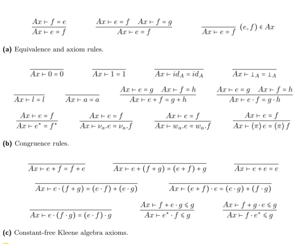
(c) Constant-free Kleene algebra axioms. Table 1 Modular deduction system
▸ Lemma 9. For any subset of expressions S chosen from{T, U, E ⟨A⟩ , E ⟨L⟩ , E+, C}, for
any permutation π, and for any expression e∈ E, e ∈ S ⇔ π & e ∈ S. Furthermore, if e has the type A then π& e ∶ π (A), and if a is fresh for e then π (a) # π & e.
(Note the equivalence in the first point, which is why we keep a residual empty permutation when we apply a permutation to an expression of the shape⟨π⟩ e.)
2.3
Proofs
A generic framework for proofs
We now describe a generic framework for defining equational theories over E. Given a relation
Ax⊆ E × E, we define the judgement Ax ⊢ e = f to hold if it can be inferred in the system
displayed in Table 1 (where Ax⊢ e ⩽ f is a shorthand for Ax ⊢ e + f = f). Notice that we have “hardwired” some laws of Kleene Algebra (KA) in this system, on the basis that they should hold for any reasonable equational system for Nominal Kleene Algebra. However, as we have two sets of constants, we cannot put inside the generic system the Kleene Algebra laws dealing with them. For instance when we consider expressions over the untyped syntax, the fact that e⋅ 1 = e will be stated inside Ax. It is a simple matter to check that whatever
Sets of axioms
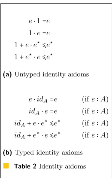
In Tables 2-6, we present a number of possible sets of axioms, which may be combined to axiomatise the different subsets we consider. All the axioms displayed here are implicitly universally quantified.
The first groups of axioms correspond to the axioms of KA for 1, declined in a typed and an untyped fashion. We then do the same for 0 andA, first with the KA axioms, and then for its interactions with⟨π⟩, νa and wa, always separating between the typed and untyped cases. These sets of axioms for constants are presented in Tables 2 and 3.
We then introduce sets of axioms to handle permutations. The axiom propagating wa is set apart, as it only makes sense for typed expressions. This group is displayed in Table 4. Notice that no law speaks about zeros, as it already has been dealt with in (3a).
The sets of axioms in Table 5 are simple distributive laws of the restriction and weakening operators. The next group, displayed in Table 6, constitutes the core of the nominal theory of expressions. The untyped axioms are mostly the classic nominal axioms, taken from [6]. The only new axiom here is (6b), where we use syntactic permutations rather than semantic ones. The typed axioms are for the most part straightforward reformulations of the previous ones. Notice that in the typed case, we do not need to use freshness conditions, but rather typing statements. The last law of the set (6f) reflects the fact that for an untyped expression
e, if a≠ b then a # e ⇔ a # νb.e.
2.4
Theories
A theory is given by a relation Ax, listing the axioms, and a set S from which we take expressions. As expressions may be typed or untyped, atomic or literate, clean or not and positive or not, there are 16 theories, listed in Table 7.
Notice that every subset of expressions mentioned in this table is associated with a single theory. In the following, for concision, we may refer to a theory by simply giving its base set. It is also worth mentioning that for every set S, the theories for E ⟨L⟩ ∩ S and E ⟨A⟩ ∩ S use the same set of axioms.
The theory E ⟨A⟩ ∩ U ∩ C corresponds precisely to the axiomatisation of NKA given in [6]. In our view, the best theory for defining the interpretation of a program would be E+⟨L⟩ ∩ U ∩ C, but a relational interpretation is best defined in E+⟨L⟩ ∩ T.
A difficulty is that if we have a theory(S, Ax), with two expressions e, f ∈ S such that
Ax⊢ e = f, it may be the case that the proof uses expressions outside of S. This is generally
what happens in systems with 0 (or A): if e∉ S and 0 ∈ S, then:
Ax⊢ 0 = 0 ⋅ e Ax⊢ 0 ⋅ e = 0 Ax⊢ 0 = 0
This is a bad property when one wants to prove results by structural induction on proofs. This phenomenon disappears with stable theories:
▸Definition 10. A theory(S, Ax) is stable if for any expressions e, f ∈ E such that Ax ⊢ e = f,
e∈ S if and only if f ∈ S.
e⋅ 1 =e
1⋅ e =e 1+ e ⋅ e⋆⩽e⋆ 1+ e⋆⋅ e ⩽e⋆
(a) Untyped identity axioms
e⋅ idA=e (if e∶ A)
idA⋅ e =e (if e∶ A)
idA+ e ⋅ e⋆⩽e⋆ (if e∶ A)
idA+ e⋆⋅ e ⩽e⋆ (if e∶ A) (b) Typed identity axioms
Table 2 Identity axioms
e+ 0 =e
e⋅ 0 =e (if e∈ U) 0⋅ e =e (if e∈ U) ⟨π⟩ 0 =0
νa.0=0
(a) Untyped zero axioms
e+ A=e (if e∶ A) e⋅ A=e (if e∶ A) A⋅ e =e (if e∶ A) ⟨π⟩ A=π(A) νa.A=A∖{a} (if a∈ A) wa.A=A∪{a} (if a∉ A) (b) Typed zero axioms
Table 3 Zero axioms
⟨π⟩ (e + f) = ⟨π⟩ e + ⟨π⟩ f ⟨π⟩ (e ⋅ f) = ⟨π⟩ e ⋅ ⟨π⟩ f ⟨π⟩ (e⋆) = (⟨π⟩ e)⋆ ⟨π⟩ (νa.e) =νπ(a).⟨π⟩ e ⟨π⟩ ⟨π′⟩ e = ⟨π ○ π′⟩ e ⟨π⟩ 1 =1 ⟨π⟩ idA=idπ(A) ⟨⎧⎩⎫⎭⟩e =e ⟨π⟩ a =π (a) (if a ∈ A) ⟨π⟩ l =π (l) (if l ∈ L) (a) General permutation axioms
⟨π⟩ (wa.e) =wπ(a).⟨π⟩ e
(b) Permutation vs. wa
Table 4 Permutation axioms
wa.(e + f) =wa.e+ wa.f
wa.(e⋆) = (wa.e⋆)
wa.(e ⋅ f) =wa.e⋅ wa.f
wa.(idA) =idA∪{a} (if a∉ A)
wa.(wb.e) =wb.(wa.e) (a) Weakening
νa.(e + f) =νa.e+ νa.f
νa.(νb.e) =νb.(νa.e) (b) Restriction
νb.e=νa.⎧⎩a b⎫⎭ & e (if a # e) (a) Untyped α-conversion with&
νb.e=νa.⟨⎧⎩a b⎫⎭⟩e (if a # e) (b) Untyped α-conversion with⟨π⟩
νb.e=νa.⎧⎩a b⎫⎭ & e (if νb.e∶ A and a ∉ A) (c) Typed α-conversion with&
νb.e=νa.⟨⎧⎩a b⎫⎭⟩e (if νb.e∶ A and a ∉ A) (d) Typed α-conversion with⟨π⟩
νa.e=e (if a # e)
νa.f⋅ e =νa.(f ⋅ e) (if a # e)
e⋅ νa.f =νa.(e ⋅ f) (if a # e) (e) Untyped nominal axioms
νa.wa.e=e (if νa.wa.e∶ A) (νa.f) ⋅ e =νa.(f ⋅ wa.e)
e⋅ (νa.f) =νa.(wa.e⋅ f)
νb.wa.e=wa.νb.e (if a≠ b) (f ) Typed nominal axioms Table 6 Nominal axioms
Name Set Axioms
NKAmpu E+⟨L⟩ ∩ U
(2a) (4a) (5b) (6b) (6e)
NKAspu E+⟨A⟩ ∩ U
NKAnmpu E+⟨L⟩ ∩ U ∩ C
(2a) (5b) (6a) (6e)
NKAnspu E+⟨A⟩ ∩ U ∩ C
NKAmu E ⟨L⟩ ∩ U
(2a) (3a) (4a) (5b) (6b) (6e)
NKAsu E ⟨A⟩ ∩ U
NKAnmu E ⟨L⟩ ∩ U ∩ C (2a) (3a) (5b) (6a) (6e)
NKAnsu E ⟨A⟩ ∩ U ∩ C NKAmpt E+⟨L⟩ ∩ T (2b) (4a) (4b) (5a) (5b) (6d) (6f) NKAspt E+⟨A⟩ ∩ T NKAnmpt E+⟨L⟩ ∩ T ∩ C (2b) (5a) (5b) (6c) (6f) NKAnspt E+⟨A⟩ ∩ T ∩ C NKAmt E ⟨L⟩ ∩ T (2b) (3b) (4a) (4b) (5a) (5b) (6d) (6f) NKAst E ⟨A⟩ ∩ T NKAnmt E ⟨L⟩ ∩ T ∩ C (2b) (3b) (5a) (5b) (6c) (6f) NKAnst E ⟨A⟩ ∩ T ∩ C Table 7 Theories
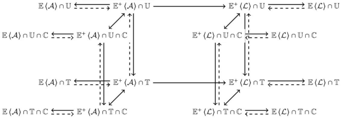
E+⟨L⟩ ∩T E+⟨L⟩ ∩U E ⟨L⟩ ∩ T E ⟨L⟩ ∩ U E+⟨L⟩ ∩T ∩ C E+⟨L⟩ ∩U ∩ C E ⟨L⟩ ∩ T ∩ C E ⟨L⟩ ∩ U ∩ C E+⟨A⟩ ∩T E+⟨A⟩ ∩U E ⟨A⟩ ∩ T E ⟨A⟩ ∩ U E+⟨A⟩ ∩T ∩ C E+⟨A⟩ ∩U ∩ C E ⟨A⟩ ∩ T ∩ C E ⟨A⟩ ∩ U ∩ C
Figure 1 The two cubes as sets
3
Ordering theories
3.1
Definitions
We define two preorders to compare theories. The first one is the strongest one:
▸ Definition 11 (Embedding preorder). A theory (S, Ax) can be embedded into (S′, Ax′),
written(S, Ax) ≼ (S′, Ax′) if there is a function φ such that for any e ∈ S, φ (e) ∈ S′, and for any e, f ∈ S, Ax ⊢ e = f ⇔ Ax′⊢ φ (e) = φ (f). In that case we say that φ is an embedding
of(S, Ax) into (S′, Ax′).
When a theory can be embedded into a second one, then every model of the latter one gives rise to a model former one. However, some intuitively equivalent theory cannot be compared using this preorder. For instance, E+⟨A⟩ ∩ T cannot be embedded into E+⟨A⟩ ∩ U. Indeed, while the typed expressions id{a}and id{a,b}are not equal (they have different types), they have the same untyped behaviour and both of them should be mapped to the untyped constant 1. To this end, we introduce a slightly weaker preorder:
▸Definition 12 (Reduction preorder). A theory(S, Ax) reduces to (S′, Ax′), which we denote
by(S, Ax) ≪ (S′, Ax′), if for any pair (e, f) ∈ S × S there is a pair of expressions (e′, f′) ∈ S′
such that Ax⊢ e = f ⇔ Ax′⊢ e′= f′.
▸Lemma 13. If (S, Ax) ≪ (S′, Ax′) and if (S′, Ax′) is decidable, then so is (S, Ax).
▸Remark. This lemma assumes an effective proof of(S, Ax) ≪ (S′, Ax′): there must be a
way to build the pair e′, f′ from the pair e, f . Our (Coq) proofs below have this property.
3.2
Embeddings
We summarise the results we obtained using Coq on Figure 1. (The scripts are available online [1]). A plain arrow is drawn between two theories if the source of the arrow can be embedded into the target of the arrow, and a dashed arrow when the source reduces to the target. Thanks to the decidability result for E ⟨A⟩ ∩ U ∩ C [5], this ensures that all atomic theories are decidable.
We discuss in more details how we obtained some of these results.
3.2.1
Reducing to positive fragments
The first step consists in getting rid of the constants 0 andA, so that we can focus on stable theories (Definition 10). We only present here the untyped case. In other words we choose a
theory(S, Ax), with S taken from the set {E ⟨A⟩ ∩ U, E ⟨A⟩ ∩ U ∩ C, E ⟨L⟩ ∩ U, E ⟨L⟩ ∩ U ∩ C}, the corresponding positive theory being(S ∩ E+, Ax∖ (3a)).
▸Definition 14. If e is an untyped expression, extract(e) is the unique normal form of e
with respect to the following confluent rewriting system:
e+ 0 → e 0+ f → f e⋅ 0 → 0 0⋅ f → 0 νa.0→ 0 ⟨π⟩ 0 → 0 0⋆→ 1. The interesting property of this function is that if Ax⊢ e = 0, then extract (e) is syntactically equal to 0, and extract(e) ∈ E+otherwise. Furthermore, for every e∈ S, Ax ⊢ extract (e) = e. The formal proof then relies on two key observations:
1. If(e, f) ∈ Ax ∖ (3a), then Ax ∖ (3a) ⊢ extract (e) = extract (f).
2. If(e, f) ∈ (3a), then extract (e) = extract (f). This allows to prove by induction on proofs that:
Ax⊢ e = f ⇒ Ax ∖ (3a) ⊢ extract (e) = extract (f) .
Because the positive axiomatisation is included in Ax, we also get:
Ax∖ (3a) ⊢ extract (e) = extract (f) ⇒ Ax ⊢ extract (e) = extract (f) .
The fact that extract(e) is provably equal to e with the axioms Ax allows to close the proof of equivalence, with the entailment:
Ax⊢ extract (e) = extract (f) ⇒ Ax ⊢ e = f.
However, if Ax⊢ e = 0 then extract (e) ∉ E+. This means that we cannot directly use
extract() as an embedding between theories. We obtain the reduction as follows: when
given the pair e, f , we compute extract(e) and extract (f). If both of these are equal to zero, then when map the pair to equal positive expressions, say 1, 1. If both of them are non-zero, then we produce extract(e) , extract (f). Otherwise we produce different positive expressions, say 1, a in the atomic case and 1, l in the literate case.
3.2.2
From presheaves to freshness, and back
Let(S, Ax) be a positive untyped theory, meaning S ⊆ E+∩ U, and (S′, Ax′) be the
corres-ponding positive typed theory. We show here how to transport S into S′, and vice versa. This corresponds to the vertical arrows on Figure 1. The key tools in this case are the erasure and retyping functions.
▸Definition 15 (Erasure). The erasure of e∈ T, written ⌊e⌋, is the expression obtained from
e by removing all weakenings(wa), and replacing all idAwith 1 and all A with 0.
▸Lemma 16. If e∈ S′ then⌊e⌋ ∈ S, and if e ∶ A then ♮ (⌊e⌋) ⊆ A.
▸Definition 17 (Retyping). Let e∈ U, we define the retyping of e, written ⌈e⌉, by structural
induction:
⌈0⌉ ∶=∅ ⌈1⌉ ∶=id∅ ⌈e + f⌉ ∶=w♮(f)∖♮(e).⌈e⌉ + w♮(e)∖♮(f).⌈f⌉ ⌈a⌉ ∶=a ⌈l⌉ ∶=l ⌈e ⋅ f⌉ ∶=w♮(f)∖♮(e).⌈e⌉ ⋅ w♮(e)∖♮(f).⌈f⌉
⌈e⋆⌉ ∶= ⌈e⌉⋆ ⌈νa.e⌉ ∶=νa.⌈e⌉ (if a∈ ♮ (e))
⌈⟨π⟩ e⌉ ∶= ⟨π⟩ ⌈e⌉ ⌈νa.e⌉ ∶=νa.wa.⌈e⌉ (if a∉ ♮ (e)) The notation wA.e is justified by the law wa.wb.e= wb.wa.e, holding in every typed theory.
▸Lemma 18. e∈ S entails ⌈e⌉ ∈ S′. Furthermore,⌈e⌉ has the type ♮ (e).
These functions allow one to go back and forth between S and S′:
▸Lemma 19. If e∈ S, then e = ⌊⌈e⌉⌋. If e ∶ A, then:
(6f) (5a) (4b) ⊢ e = wA∖♮(⌊e⌋).⌈⌊e⌋⌉ .
Furthermore, if S⊆ C, we may remove the axiom (4b).
From this lemma, we obtain that the retyping function is an embedding of S into S′. But it also shows a problem for the other direction. For instance the expressions e and wa.e have different types, and are thus different, but they will be mapped to the same expression. For this reason, we cannot use the erasure function to embed S′ into S.
Nevertheless, we can use it to show that S′is simpler than S. Given a pair of expressions
e, f∈ S′, if e and f have the same type, then we produce the pair⌊e⌋ , ⌊f⌋ which is equiprovable. If it is not the case, we purposely produce different expressions, as in the previous section.
3.2.3
From atomic to literate
We assume there is an atom α∈ A and an element λ ∈ L with ♮ (λ) = {α}. We show the transformation from E+⟨A⟩∩U to E+⟨L⟩∩U, which corresponds to the central horizontal top arrow on Figure 1. Let NKApu be the set of axioms(2a), (4a), (5b), (6b), (6e) corresponding to the theory of these sets.
▸ Definition 20 (From atoms to letters.). Given an expression e ∈ E+⟨A⟩ ∩ U, we obtain
the expression ⇃e⇂ ∈ E+⟨L⟩ ∩ U by replacing every atomic variable a by ⟨⎧⎩a α⎫⎭⟩λ. We write⇃E+⟨A⟩ ∩ U⇂ for the set of expressions f ∈ E+⟨L⟩ ∩ U, such that there is an expression
e∈ E+⟨A⟩ ∩ U such that f = ⇃e⇂.
For any expression e, e ∈ ⇃E+⟨A⟩ ∩ U⇂ if and only if each literate variable in e has the identifier x. It is also worth noting that⇃_⇂ preserves freshness: a # e ⇔ a # ⇃e⇂. As for typed and untyped expressions, we define an inverse operation.
▸Definition 21 (Going back). The inverse operation is only defined on literate expressions
whose variables carry the identifier x, and thus have a singleton support. The expression↿e↾ is then obtained by replacing every variable by the single atom in its support.
The function↿_↾ is the inverse of ⇃_⇂, ⇃_⇂ preserves NKApu-equality, and ↿_↾ preserves NKApu-equality on the image of⇃_⇂.
▸Lemma 22. ∀e ∈ E+⟨A⟩ ∩ U, NKApu ⊢ e = ↿⇃e⇂↾.
▸Lemma 23. ∀e, f ∈ E+⟨A⟩ ∩ U, NKApu ⊢ e = f ⇒ NKApu ⊢ ⇃e⇂ = ⇃f⇂.
▸Lemma 24. ∀e, f ∈ E+⟨L⟩ ∩ U ∩ ⇃E+⟨A⟩ ∩ U⇂, NKApu ⊢ e = f ⇒ NKApu ⊢ ↿e↾ = ↿f↾.
By putting all together, we obtain that⇃_⇂ is an embedding of E+⟨A⟩ ∩ U into E+⟨L⟩ ∩ U.
4
Relational interpretation of literate expressions
Our main motivation for developing the typed syntax was to define a relational interpretation of expressions. As explained in the introduction, the classical way of interpreting a program as a relation is to consider memory states as functions, associating values to memory cells. A
program is then simply a relation between memory states. Furthermore, in most high level programming languages, one cannot access every part of the memory: a variable should be declared before it is used. There are also constructs allowing one to declare a local variable, which is hidden from the rest of the program. Both of these considerations can be encoded by considering functions with a finite domain: the set of memory locations that are visible in the current scope.
Let us be more precise. Consider that the setA of atoms corresponds to memory locations, and that locations may contain values from an arbitrary setV. A memory state of domain
A∈ ℘f(A) is then a function from A to V, and an expression of type A will be interpreted as a binary relation over memory states of domain A (whence the presheaf structure).
Regular operations are interpreted using the standard operations on binary relations; in particular, idA is interpreted as the identity relation on VA. To interpret letters, we need to fix an equivariant map φ that assign to a letter x a relation between memory states with domain ♮ (x). Several choices are possible for the operations of restriction (νa) and weakening(wa), yielding slightly different theories. Here is a possibility which gives rise to a model of our theory: if R is a relation overVA, then we define
νa.R∶= {(f↾A, g↾A) ∣ (f, g) ∈ R} ; (if a∈ A)
wa.R∶= {(f, g) ∣ (f↾A, f↾A) ∈ R and f(a) = g(a)} . (if a∉ A) (Where f↾A is the restriction of a function f∈ VB for some superset B of A.)
Note that this model is not free: for all relations R, S we have νa.(R ⋅ S) ⊆ (νa.R) ⋅ (νa.S), which is not an inequation provable from the axioms.
Example.
Consider the program swap(x, y) that exchanges the contents of the variables x and y. The natural implementation of this program is the following: let t in t← x; x ← y; y ← t.
The instruction x← y may be represented by a nominal element assign (x, y) with support {x, y}, and such that π (assign (x, y)) = assign (π (x) , π (y)). Accordingly, the program swap is represented by the following expression, where the location is hidden using a top-level restriction.
νt.(assign (t, x) ⋅ assign (x, y) ⋅ assign (y, t)) .
Alternatively, one can obtain an expression with a single letter using explicit permutations: let a1 and a2 be two atoms, and set a ∶= assign (a1, a2). The instruction x ← y may be represented by⟨⎧⎩x a1⎫⎭⎧⎩y a2⎫⎭⟩a, and the program swap by
νt.(⟨⎧⎩t a1⎫⎭⎧⎩x a2⎫⎭⟩a) ⋅ (⟨⎧⎩x a1⎫⎭⎧⎩y a2⎫⎭⟩a) ⋅ (⟨⎧⎩y a1⎫⎭⎧⎩t a2⎫⎭⟩a).
5
Future work
We leave two questions for future work. First, is it possible to reduce the literate theory of nominal Kleene algebra to that of atomic nominal Kleene algebra? If not, is there a free language theoretic model for which we could obtain decidability?
Second, is there a free relational model for our literate theory?
Acknowledgements.
We would like to thank Daniela Petrisan and Alexandra Silva for the discussions that have led to this work.
References
1 Paul Brunet. Web appendix to this abstract, 2016. http://perso.ens-lyon.fr/paul. brunet/nka.
2 Murdoch Gabbay and Andrew Pitts. A new approach to abstract syntax involving binders. In Logic in Computer Science, 1999. Proceedings. 14th Symposium on, pages 214–224. IEEE, 1999.
3 Murdoch James Gabbay and Vincenzo Ciancia. Freshness and name-restriction in sets of traces with names. In Foundations of Software Science and Computational Structures,
FoSSaCS 2011, pages 365–380. Springer, 2011.
4 Dexter Kozen. Kleene algebra with tests. Transactions on Programming Languages and
Systems, 19(3):427–443, May 1997. doi:10.1145/256167.256195.
5 Dexter Kozen, Konstantinos Mamouras, Daniela Petrisan, and Alexandra Silva. Nominal Kleene Coalgebra. In Automata, Languages, and Programming, ICALP 2015, pages 286– 298. Springer, 2015.
6 Dexter Kozen, Konstantinos Mamouras, and Alexandra Silva. Completeness and incom-pleteness in Nominal Kleene Algebra. In Relational and Algebraic Methods in Computer
Science, RAMiCS 2015, pages 51–66. Springer, 2015.
7 Andrew M Pitts. Nominal Sets: Names and Symmetry in Computer Science, volume 57. Cambridge University Press, 2013.