Constraint-aware distributed robotic assembly and disassembly

Constraint-Aware Distributed

Robotic Assembly and Disassembly

by

Timothy Ryan Schoen

ARCHNES

Submitted to the Department of Electrical Engineering and Computer Science

in partial fulfillment of the requirements for the degree of

Master of Engineering in Electrical Engineering and Computer Science at the

MASSACHUSETTS INSTITUTE OF TECHNOLOGY

June 2012

@

Timothy Ryan Schoen, MMXII. All rights reserved.

The author hereby grants to MIT permission to reproduce and to distribute publicly paper and electronic copies of this thesis document in whole or in

part in any medium now known or hereafter created.

Author ... .

.. .. .. .. .. .. .. .. ..

..

.

Department of Electrical Engineering and Computer Science May 21, 2012 Certified by .... ... Daniela Rus Professor TJiesis Supervisor Accepted by...

Prof. Dennis M. Freeman, Chairman Masters of Engineering Thesis Committee

Constraint-Aware Distributed

Robotic Assembly and Disassembly

by

Timothy Ryan Schoen

Submitted to the Department of Electrical Engineering and Computer Science

on May 21, 2012, in partial fulfillment of the

requirements for the degree of

Master of Engineering in Electrical Engineering and Computer Science

Abstract

In this work, we present a distributed robotic system capable of the efficient assembly and disassembly of complex three-dimensional structures. We introduce algorithms for equitable partitioning of work across robots and for the efficient ordering of assembly or disassembly tasks while taking physical constraints into consideration. We then extend these algorithms to a variety of real-world situations, including when component parts are

unavailable or when the time requirements of assembly tasks are non-uniform. We

demon-strate the correctness and efficiency of these algorithms through a multitude of simulations. Finally, we introduce a mobile robotic platform and implement these algorithms on them. We present experimental data from this platform on the effectiveness and applicability of our algorithms.

Thesis Supervisor: Daniela Rus

Acknowledgements

I would like to thank the Boeing Corporation for sponsoring this research, and Daniela Rus

for her advice and guidance over the past two years. I am indebted to the members of the

Distributed Robotics Lab, and especially to my fellow robot wranglers David Stein and Ross Knepper. Special thanks to Seungkook Yun, without whose work none of this could have been possible. And finally, I am incredibly grateful for my friends and family, who

Contents

1 Introduction 17

1.1 Motivation . . . . 17

1.2 Algorithmic Contributions . . . . 20

1.2.1 Discrete Partitioning . . . . 20

1.2.2 Constraint-Aware Ordered Assembly . . . 20

1.2.3 Ordered Assembly with Part Unavailability . . . 21

1.2.4 Ordered Assembly with Time Constraints . . . 21

1.2.5 Constraint-Aware Ordered Disassembly . . . 21

1.3 Organization of Thesis . . . 21 2 Related Work 23 3 Problem Formulation 25 3.1 Assembly . . . 25 3.2 Robots.. ... ... .. .. .. .... ... . ... .. 25 3.3 Demanding Mass . . . 26 3.4 Task Partitioning . . . 26 3.5 Assembly Ordering . . . 27

4 Discrete Equal Mass Partitioning 29 4.1 Convergence . . . 32

4.2 Runtime . . . 33

5 Delivery & Assembly with Ordering 37

5.1 Runtime . . . 44

5.2 Convergence . . . 45

6 Adaptation in Decentralized Assembly 47 6.1 Decentralized Scheduling Algorithm in the Presence of Part Supply Uncer-tainty . . . 47

6.1.1 Convergence . . . 50

6.1.2 Runtime . . . 50

6.1.3 Generalization . . . 50

6.2 Decentralized Scheduling Algorithm with Non-Uniform Assembly Times . 51 6.2.1 Convergence . . . 51

6.2.2 Runtime . . . 52

6.2.3 Generalization . . . 52

6.3 Simulations . . . 52

7 Disassembly with Part Ordering 57 7.1 Runtime . . . 60

7.2 Convergence . . . 60

8 Implementation 61 8.1 Mobile Manipulators . . . 61

8.2 Localization . . . 61

8.3 Software and Communication . . . 63

8.4 Blueprints and parts . . . 63

8.5 Navigation. . . . 67

8.6 Manipulation . . . 67

8.7 Ordering . . . 68

8.8 Delivery . . . 68

8.9 Assembly . . . 68

9 Experiments

9.1 Two-Dimensional Experimental Results . . . . 9.1.1 Overall Results . . . .

9.1.2 Runtime and Efficiency . . . .

9.2 Three-Dimensional Experimental Results: Two Robots

9.2.1 Overall Results . . . .

9.2.2 Runtime and Efficiency . . . .

9.3 Three-Dimensional Results: Four Robots . . . . 9.3.1 Overall Results . . . .

9.3.2 Runtime and Efficiency . . . . 9.4 Experimental Results with Part Unavailability...

9.5 Handoff Experimental Results . . . .

71 . . . 71 . . . 71 . . . 72 . . . 73 . . . 73 . . . 75 . . . 75 . . . 75 . . . 76 . . . 76 . . . 78

10 Conclusion and Future Work

10.1 Summary of Contributions . . . .

10.2 Future Work . . . .

79

79 80

List of Figures

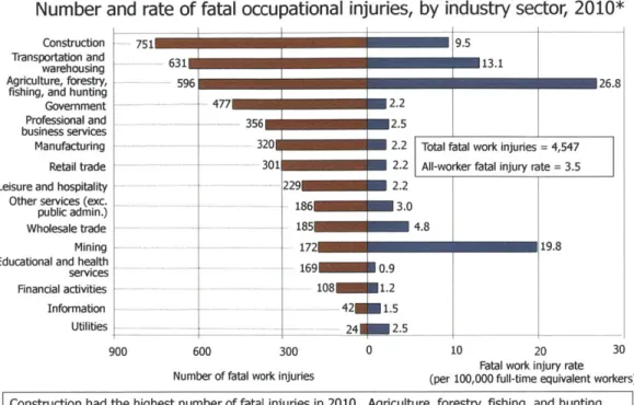
1-1 At 751 fatalities in 2010, construction results in the largest number of work-related fatalities of any industry. As reported by the U.S. Bureau of Labor Statistics. . . . . 18

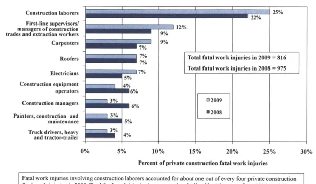
1-2 Among construction fatalities, about a quarter of the fatalities are suffered

by the construction laborers themselves. As reported by the U.S. Bureau of

Labor Statistics. . . . . 19

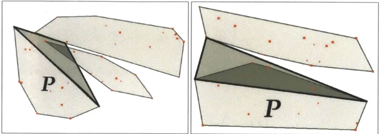
4-1 Test to identify stealable vertices. In the first image, the triangles with bold outlines mark the region that would be added to P due to a trade of a vertex. In the first case, adding the vertex would cause a collision between two polygons. In the second, the vertex under consideration would be a valid candidate to trade. . . . 31

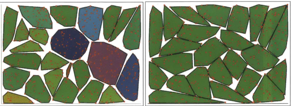
4-2 Data from running partitioning algorithm. The first image shows the initial configuration, and the second shows the partitions after 26 time-steps on a set of point-masses with random location and mass. Shade is a function of total m ass of a partition . . . 34

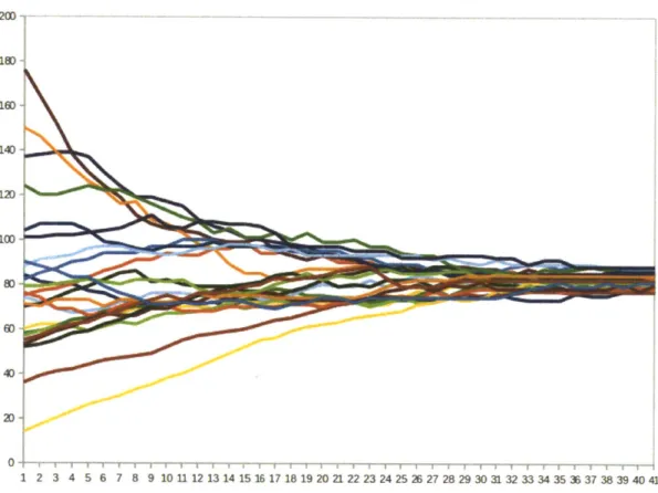
4-3 Total mass of each partition over time during a typical run of the

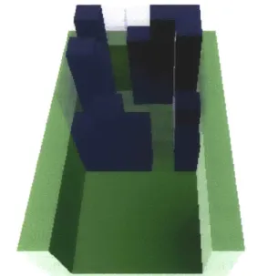
5-1 The state of the system mid-run building a hollow blue box at the end of a green hallway, with a uniform mass function. With nothing but ba-sic knowledge of the DAG the system can complete the structure, but part placement is suboptimal. Note that the front of the structure is mostly built, creating a bottleneck which limits the rate at which delivery robots can de-liver parts; and some parts of the structure are built to full height, limiting the number of assembly bots that can work simultaneously. . . . 40

5-2 The score function has the property that given two sets, the function will give a higher score to the set with most values generating the lowest value

off... 43

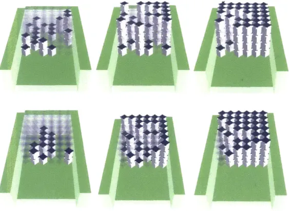
5-3 Part placement while building a solid cube using uniform mass (top) and

ordering (bottom). Note that without the ordering algorithm, work in the front occurs first (top middle), making it harder for delivery robots to reach subassemblies in the back. Also note how more of the stacks of blocks in the top right have reached their maximum height, leaving less opportunities for parallelism . . . 45 5-4 The average number of parts with positive mass across time over 50 runs of

building a solid cube at the end of a hallway with 5 assembly and 4 delivery robots, with uniform mass on placeable parts (top) and masses calculated

using the proposed algorithm (bottom) . . . 46

6-1 When the supply of a part type runs out, the assembly subtree with that part

as the root is temporarily pruned. When the part is resupplied, the subtree is added back into the overall assembly tree. . . . 49

6-2 ... ... ... 53

6-3 The average demanding mass over time of ten simulations using the

origi-nal algorithm (blue) and ten simulations using the modified algorithm (red). At t=20 the supply of plane panels is extinguished; at t=80 the supply is re-plenished. . . . 54

8-1 Side view of the KUKA YouBot. The holonomic base allows for omnidi-rectional movement, while the five d.o.f. arm provides a usable workspace in front of, to the side of, and on top of the robot. The spherical reflec-tive markers can be seen on both the base and manipulator for accurate localization. . . . . 62 8-2 System architecture and information flow. Each oval represents a separate

ROS node, and the arrows indicate messages being passed between nodes

(or in some cases, between robots). . . . . 64

8-3 Our test parts for the main algorithm, arranged in a simple two-layer "log cabin" design. Each part has a gripping area and two diamond-shaped

sup-ports, one on each end. . . . . 65

8-4 Our test parts for the part supply algorithm. Parts are divided into top parts

(red) and foundation parts (blue). Each part is a styrofoam cube with slots

cut into the top to allow the youBots to grip them. . . . . 66

8-5 Image of a delivery robot performing a delivery. Since the robots do not

have vision and the assembly parts are not tracked by the Vicon system, the handoff and communication must be precise. . . . . 69

9-1 Robot activity over time in trial 4. Solid blocks of color indicate when a robot was busy with a task, as opposed to idle. . . . 73

9-2 An assembly robot places the final part on the three-dimensional tower.

The tower is composed of six layers of the log cabin construction, or three of the simple squares from Section 9.1. This tower is the result of trial #1 from Table 9.2. . . . 74

9-3 Assembly sequence when no parts run out (top three images) and when the

top/red cubes run out after one has been placed (bottom three). Even with

the part supply running out, the robots continue to work and ultimately

List of Tables

8.1 Summary of differences between our theoretical algorithms and system

im-plem entation. . . . . 70

9.1 Summary of two-robot assembly trials for a square. . . . . 72

9.2 Summary of two-robot assembly trials for a tower . . . 73

9.3 Summary of four-robot assembly trials for a tower. . . . 75

9.4 Summary of two-robot assembly trials of stairs. In these trials, part supply never ran out. . . . 77

9.5 Summary of two-robot assembly trials of stairs. In these trials, part supply of the red parts ran out after the first placement, but was resupplied after three more placements. . . . 77

Chapter 1

Introduction

1.1

Motivation

Five million individuals in the United States are employed by the construction and extrac-tion services industry, making it an average-sized industry with about four percent of the

US workforce[l]. However, individuals in this industry suffer a disproportionate amount

of the work-related fatalities in the country; construction results in the largest number of work-related fatalities of any industry[2]. Among these fatalities, the largest portion of

them are the construction laborers themselves, the individuals performing the lowest-level construction tasks[3]. We believe that these trends extend to the other countries as well, and as such make construction a dangerous job.

Most constructions tasks require the transportation, manipulation, and precise assembly of a variety of objects, many of which may be heavy or hazardous in a variety of ways. We believe that humans are not particularly well-suited for these tasks, and propose instead the introduction of robotics to accomplish these assembly tasks. Thus we remove humans from the situations most hazardous to their health and well-being.

We acknowledge that there are many components of assembly for which a human is much more able to complete than a robot. The solutions we propose are not intended to completely replace humans in the assembly progress, but instead to replace only the most basic and dangerous of these activities. As the field of robotics progresses, one can imagine more responsibility being allocated to the robotic platform to complete assembly activities,

Number and rate of fatal

Construction 751

Transportation and 6 warehousing

Agriculture, forestry, 596

fishing, and hunting

Government - -4771

Professional and - - ---business services

Manufacturing

Retail trade - - - - -Leisure and hospitality

Other services (exc .

public admin.) Wholesale trade

Mining - - -

-Educational and health services Financial activities Information Utilities 900 600 Number of fa

occupational injuries, by industry sector, 2010*

- ~ ~95 13.1 1

-

-

1 I 26.8 356K 3201 -301 229 186 185 172 169 300 al work injuries E 2.2 M2.5

K 2.2 Total fatal work injuries = 4,547

K 2.2 All-worker fatal injury rate = 3.5

K 2.2 3.0 4.8 -19.8 108 421 - 241 0.9 1.5 2.5 0 10 20 30

Fatal work injury rate (per 100,000 full-time equivalent workers) Construction had the highest number of fatal injuries in 2010. Agriculture, forestry, fishing, and hunting sector had the highest fatal work injury rate.

*Data for 2010 are preliminary.

NOTE: All industres shown are private with the exception of government, which ndudes fatalities to workeis employed by governmental orgazat ons regardless of industry. Fatal injury rates exdlude workers under the age of 16 years, volunteers, and resident military. The number of fatal work injuries represents total published fatal injuries before the exclusions. For additional information on the fatal work injury rate methodology changes please see htto://www~bs.ovliifloshnotice10.htm 16

SOURCE: U.S. Bureau of Labor Statistics, U.S. Department of Labor, 2011.

Figure 1-1: At 751 fatalities in 2010, construction results in the largest number of work-related fatalities of any industry. As reported by the U.S. Bureau of Labor Statistics.

but still being supervised by skilled human workers.

One approach to robotic construction is a centralized controller that completes the as-sembly task in a predefined order. This approach has a number of drawbacks. The ef-ficiency and parallelism is limited, in the sense that the tasks are completed in a serial manner. In the case of multiple robots receiving commands from a centralized controller, parallelism increases but there is a lack of scalability. As the number of robots increases the complexity of processing and communication for the centralized controller grows quickly.

A centralized approach is also not adaptable to many types of failure or disturbance. A fatal

failure in the central controller would halt the assembly process regardless of the number of robots involved. A shortage of a particular part type could equally freeze the serial assembly process.

Distribution of fatal work injuries by selected occupations in the private construction industry, 2008-2009*

Construction laborers 2%

First-line supervisors/!2 2

manerf construction

trades and extraction workers 9%

Carpenters 9%

Roofers 7% Total fatal work injuries in 2009 = 816 E % Total fatal work injuries in 2008 = 975

Electricians -7

Construction equipment

operators 6%

0200 Construction managers _{3% 6%}

Painters, construction and 3% U2008

maintenance 5%

Truck drivers, heavy 3% and tractor-trailer

0% 5% 10% 15% 20% 25% 30%

Percent of private construction fatal work injuries

Fatal work injuries involving construction laborers accounted for about one out of every four private construction fatal work injuries in 2009. Total fatal work injuries in construction declined by 16 percent from 2008 to 2009. *Data for 2009 are preliminary. Data for prior years are revised and final.

SOURCE: U.S. Bureau of Labor Statistics, U.S. Department of Labor, 2010. 20

Figure 1-2: Among construction fatalities, about a quarter of the fatalities are suffered by the construction laborers themselves. As reported by the U.S. Bureau of Labor Statistics.

central to the future of manufacturing. To that end, our work has focused on developing and implementing these algorithms. We imagine a team of n robots working cooperatively to construct a given structure. We divide these robots into two classes. The first class, part delivery robots, are specialized for retrieving parts from a source location or repository and delivering them to the second class of robots. This second class, the assembly robots, are specialized for performing the assembly task given the parts delivered to them. These assembly tasks could be placing a part, bolting pieces together, applying adhesive, or any localized assembly task.

Each of the assembly robots is given a blueprint of the target structure, but beyond that the processing, control, and communication are completely decentralized. This presents several unique algorithmic challenges. The robots must decide amongst themselves how to partition the assembly work in a way that is equitable and maximizes parallelism. Given

these partitions, the robots must then decide how to sequence their order of operations, again to maximize efficiency and parallelism. Each robot must also be capable of respond-ing to disturbances -for example, the failure of a neighbor robot or the shortage of a part

supply.

We present algorithmic solutions to these challenges in a provably correct manner, while maintaining several desirable properties. We then implement our algorithms on a robotic platform to demonstrate their practicality in manufacturing tasks.

1.2 Algorithmic Contributions

The work presented in this paper builds on a body of knowledge developed at MIT and other institutions regarding the efficient construction of structures using teams of distributed robots. Specifically, it extends the work of Seungkook Yun and David Stein to make the set of assembly algorithms more robust. The main contributions of this work are as follows.

1.2.1

Discrete Partitioning

As many of the algorithms presented require the equal-weight partitioning of assembly tasks, we first present a novel algorithm to partition a set of discrete point-masses into equal partitions.' This allows the body of work available in a construction process to be equally partitioned across a team of robots, such that each can work efficiently and the overall goal can be completed in the least amount of time. The algorithm is extendable to any dimensionality, although we envision most applications in two or three dimensions.

1.2.2 Constraint-Aware Ordered Assembly

The work of Yun et al. addressed how to efficiently assemble arbitrary structures given a blueprint, but the resulting assembly order disregarded the physical constraints the struc-ture. We present an algorithm that considers these physical constraints, and develops an 'This is taken from previous work, "Constraint-Aware Coordinated Construction of Generic Structures"

assembly order designed to maximize parallelism and reduce bottlenecks in the task.2

1.2.3 Ordered Assembly with Part Unavailability

The above assembly algorithm is then adapted to account for the fact that some parts re-quired for assembly may not be always present. We present an adaptation to the algorithm

that continues to maximize robot parallelism in the face of part shortages.

1.2.4 Ordered Assembly with Time Constraints

The above assembly algorithm is again adapted to consider the fact that all assembly

op-erations are not equal. Some may be more complex than others, requiring more time to

complete. Our algorithm takes these timing parameters into consideration when

schedul-ing tasks, such that the structures are assembled in the most efficient manner.

1.2.5

Constraint-Aware Ordered Disassembly

Occasionally construction tasks are needed to build temporary structures, such as a scaf-folding of trusses used to support another assembly. These structures must be disassembled

after their purpose is complete, to clear the construction area and recycle the parts used in the structure. We present a novel algorithm for the ordering of tasks required to

disassem-ble an arbitrary structure, again considering the physical constraints of such a disassembly process.

1.3

Organization of Thesis

The first three chapters describe the challenges this thesis attempts to solve, as well as their importance and context in the manufacturing industry. Chapter 4 describes our algo-rithm for discrete partitioning of work among robots, and then Chapters 5 and 6 describe

the ordering algorithms used to maximize parallelism and efficiency in the assembly tasks.

2

This is taken from previous work, "Constraint-Aware Coordinated Construction of Generic Structures"

Chapter 7 then uses the principles described so far to develop algorithms for efficient dis-assembly. A robotic platform is described in Chapter 8, and then the results of experiments with our algorithms on this platform are presented in Chapter 9. Finally, conclusions and possibilities for future work are described in Chapter 10.

Chapter 2

Related Work

Our work builds on prior research on robotic construction and distributed coverage. A sim-ple distributed 3D construction algorithm is described by Theraulaz[5], while Werfel[6]

describes a 3D construction algorithm for modular blocks in a distributed setting. Fahlman

describes a system for planning how to build a structure using simple parts[7].

Stochas-tic algorithms for roboStochas-tic construction with dependency on raw materials are analyzed

by Matthey[8]. Three-dimensional construction with consideration to physical constraints

such as gravity and stacking was achieved by [9].

Ayanian and Kumar developed a decentralized feedback controller for a team of robots to navigate around obstacles[10]. Stochastic policies for parallel task allocation in robotic swarms were investigated by [11]. [12] developed methods for evaluating the complexity of structures, as it applies their distributed robotic construction.

The U.S. Air Force detailed their early efforts of robotic construction in [13]. Parker

et al. described a system for nest construction using a team of robots[14]. Human-robot

cooperation for construction of heavy items was explored by Lee, et al.[15] A coordinated robotic lego construction experiment was described by Schuil[16]. Stroupe et al. pre-sented a heterogeneous robotic assembly system designed to maximize a number of cost metrics[17]. Our previous work on robotic construction includes Shady3D [18] utilizing a passive bar and an optimal algorithm for reconfiguration of a given truss structure to a

target structure[ 19], and experiments in building truss structures[20].

deploy robots for coverage was originally proposed by Cortez et al.[22] and has been extended several times since then for tasks such as adaptive coverage[23] and equitable partitioning [24]. Pavone et al. described a method of distributed equitable partitioning[25]. Maini et al. explored a genetic graph partitioning algorithm[26], and Leland and

Hendrick-son presented a study of several load balancing algorithms, in this case for parallel com-puting but as could be applied to other uses[27]. Durham et al. presented a decentralized algorithm for creating Voronoi partitions among robots with pairwise communication[28]. Our recent work extends the idea of equitable partitioning and combines it with coordinated construction of truss structures[29], locational optimization[30], and adaptation to failure and shape change[3 1].

Our approach utilizes previous work on computation using barycentric coordinates[32] and convex hulls[33]. Our early algorithms were implemented on a team of robots by Bolger, demonstrating the early practicality of our approaches[34].

Chapter 3 .

Problem Formulation

In this work, we address the challenge of utilizing a team of robotic mobile manipulators

to construct a fixed assembly.

3.1 Assembly

We define an assembly to be a collection of parts connected to each other, creating a single structure. A blueprint defines the relative locations of each of these parts, as well as the nature of the parts, how they are connected to each other, and which parts have physical or reachability dependencies on each other. In this work, we assume that all structures are fixed; that is, after a part has been connected to an assembly, it will not be moved further.

Under this definition and assumptions a multitude of structures can be assembled, rang-ing from very simple two-party assemblies to complicated three-dimensional shapes such

as arches, pyramids, or furniture.

3.2

Robots

We are given a team of robots, some of which specialize in the assembly of components parts into the more complicated structure -we call these the assembly robots. The rest of the robots specialize in retrieving parts from a part cache and delivering them to the assembly robots - _{these in turn are called delivery robots. These robots are mobile, relatively small,}

and have communication capabilities with their closest neighbors. They can manipulate parts and their surroundings with manipulators of any type, including the possible use of external tools or the assistance of humans.

The team of robots is completely decentralized. There is no central robot or sched-uler determining the assembly order or issuing commands to the robots. Each robot acts independently and determines on its own best course of action to take.

3.3 Demanding Mass

We define a function

#(v)

over the assembly space, which we refer to as the demanding

mass. For each part v, the demanding mass indicates the priority of that part. The robots

utilize this mass function to determine the highest priority parts to place onto the assembly. In prior work the demanding mass function was smoothed so as to be continuous; in this work, the demanding mass function will be comprised of a delta function at the location of each part, and zero elsewhere.

3.4 Task Partitioning

In order to maximize parallelism, we follow the work of Yun et al. and divide the partition the demanding mass function into sections assigned to each robot[29]. There is exactly one partition per assembly robot, and each partition contains zero or more point masses representing parts that have not yet been assembled. We require that the partitions be convex and non-overlapping; each unassembled part is assigned to exactly one partition. Given this formulation, we would like partitions to have equal mass so that the work is equitable between robots and the overall structure is completed in the most efficient way possible.

The high-level description of our algorithm is as follows. Given the starting positions of the robots, we initially create a Voronoi partitioning of the parts. We calculate the convex hulls of each robot's partition. The robots then communicate with their neighbors to trade vertices on their hulls to create equal-work partitions. As we show, this is guaranteed to

converge to a local maximum.

3.5

Assembly Ordering

We assume that the blueprint provides information about the physical dependency and

reachability constraints of the structure, as will be defined later. We represent this

informa-tion in the form of two directed acyclic graphs (DAGs), G, = (V, E,) and G, = (V, E,). The nodes of the graphs represent the parts to be assembled, and the edges represent de-pendencies. The edges of the reachability graph point from parts that could be blocked

by other parts to those blocking parts. The edges of the physical dependency graph point

from parts that provide support to the parts they support. Under this formulation, edges

point from parts that will be assembled earlier in the assembly process to parts that will be assembled later.

These requirements, while providing a few hard constraints about the order of assembly

process, still leave a large amount of flexibility. Instead of assembling parts in a random

order within these constraints, we would like to optimize our ordering to maximize

par-allelism and reduce bottlenecks. That is, at any point, we would like a robot to decide deterministically which part it will next assemble in order to maximize a parallelism

Chapter 4

Discrete Equal Mass Partitioning

In our problem formulation we represent each part in the target structure as a point, which

is reasonable given the discrete nature of parts. We define the demanding mass of a part as a measure of its priority in placement order, where the mass of a part is 0 if a part is unplaceable or already placed and positive otherwise (this is discussed in more detail in Chapter 5). By partitioning based on this mass function, we can allocate roughly the same amount of reachable, actionable work to each robot. We repeat this algorithm continuously during runtime to maintain an equitable partitioning of the workspace

Q

as masses change dynamically while the structure is built.

A trade-off of the significant increase in fidelity we get by updating our model from a

geometry to a blueprint is a change in the nature of the density of the

Q.

The density of

Q

is used by most coverage algorithms, including canonical Lloyd algorithms for

equipar-titioning, to perform gradient descent to converge to equal-mass partitions. Our blueprint

forces the density of

Q

to be a dynamic summation of scaled Dirac delta functions, which has a gradient of either zero or infinity at all points, meaning we can not use the class of deployment algorithms that depend on Voronoi partitioning.

Vertex swap, which we present as a potential solution to this problem in [30], works

on a graph rather than in R", and requires multi-hop communication. In order to use this

algorithm, we need to define a graph that connects the set of positive mass points. If we create a relatively sparse graph we introduce unnecessary assumptions which limit which points can be in the same partition. If we create a well-connected graph we introduce the

assumption of excessively large communication radii as neighbors are defined by edges in the graph rather than L distance. We have developed a equipartitioning algorithm that does not require a graph connecting points, uses only local communication, and has lower complexity than vertex swap.

We identify partitions that are spatially compact and approximately equal mass, but as stated above Voronoi partitioning and vertex swap are not viable options. The problem of partitioning a set of point masses in R4 into non-intersecting, convex, equal-mass partitions is NP-hard, even in R2. We present the hull vertex swap algorithm (Algorithm 1), an

efficient distributed method for approximating equal-mass partitioning using only single hop communication.

Hull vertex swap converges to a convex partitioning of the points v C V distributed

across the space

Q

into a set of partitions. We allow each partition Pi, i E [1, n] to "steal"

points from its set of neighbors VpN. The focus of the algorithm is to determine which vertices can be transferred from one partition to another without creating an intersection between the convex partitions, and which vertices can be stolen to effectively converge to a solution that locally maximizes our measure of equality.

We now discuss how to determine which vertices can be stolen without introducing intersections between partitions. We then present how to compute which vertex is best to steal, if any, and finally present a proof of convergence and data from simulation. To compute which vertex to steal, each robot first computes the convex hull of its partition P; then for each vertex vi in the hulls of its neighbors, it considers the region that would be added to the polygon defined by the convex hull of P if vi were moved into P. Any vi that would not create an intersection between two polygons if added to P is considered

a stealable vertex. The area added to the region can be quickly tested for intersection by

finding the triangle formed by the tangent rays between P and vi and testing the edges of each of the hulls in

Np

for intersection with that triangle (see Figure 4-1). In higher dimensional cases this extends to the pyramid formed by tangent planes.

func-Figure 4-1: Test to identify stealable vertices. In the first image, the triangles with bold outlines mark the region that would be added to P due to a trade of a vertex. In the first case, adding the vertex would cause a collision between two polygons. In the second, the vertex under consideration would be a valid candidate to trade.

Algorithm 1 Partitioning Algorithm 1: Deploy into

Q

at random pose pi

2: P +- {v1(

lpose(v)

-pi I < Ipose(v) - pI|)Vj i}

3: loop

4: compute convex hull of P

5: update Nrp

6: X +- {v Iv E Np, v is stealable}

7: i +-- argmax(AWr, (vi)) viEX

8: if A~p(vi) > 0 then

9: communicate to NM : vi e Pu, to remove vi

10: P <- P U vi

11: end if

tion. Given that each vertex v has a mass

4(v):

MP E O

4(v)

(4.1)

vEP

INQ = Mm, (4.2)

ie[1,n]

Without loss of generality, if we consider moving a vertex v from P1 to P2, we can compute

the change in mass:

A Q=

(17

M ) (Mr2 + 4(v)) (M-4( - - Ro (4.3)

Af= Me (MlMr2 + 4(v) (Me1 - Mr2 - 4(v))) - (4.4)

Af MP, 4(v) (Me1 -M2 - 4(v)) (4.5)

When comparing two potential exchanges of vertices, we only need knowledge of the partitions that will change in order to compute both the sign and relative magnitude of our deltas. We therefore need only local knowledge to determine which vertex, if any, is best to trade. We can therefore compute a scaled local AWg of moving some v from some neighbor's partition Pi to Pe1f with:

A11N = Mpk p(v)(Mpi - MPsef - p(v)) (4.6)

(PA~jAPk#APi/

~ M~ (4.7)

4.1

Convergence

Proof 1 We know that the denominator in equation 4.7 will be unchanged by a vertex being stolen and that therefore

argmax(AWy(P +- vi)) = argmax(ANQ(P +- vi)) (4.8)

vieX viEX

so each stolen vertex will result in an increase in H Q. The value of W is bounded from above and all | ANI is bounded from below, so by induction the algorithm must converge to a local maximum.

4.2

Runtime

Theorem 2 The update at each step of Algorithm 1 runs in 0(||| + I N I I

I

P

) time.

Proof 2 Consider a single step of Algorithm ] running on a robot in R d. Finding a trian-gle or cone takes 0(1 P1) time. Checking for intersections takes 0(N || d-1). This check needs to be run on 0(1 A ) candidate points [33]. Computation of each AN takes con-stant time, so the computation of candidate points dominates this function. The runtime per

step is therefore 0(||I|(||\|- +( ||p|}

)

=

0(|II|Id

- I

IM IIIPI ).

Because only the hull is considered, this is often much faster in practice.

4.3

Simulations

We ran the partition algorithm on several hundred randomly generated sets of pointmasses with random mass. Point location was sampled from either a uniform distribution or 2D Gaussian. The partition masses converged on all pointsets such that their standard devia-tion was less than twice the average mass of a point. No partidevia-tionings contained outliers after convergence, which suggests that most local maxima are good approximations of equal-mass partitioning (see Figures 4-2 and 4-3). The simulations took 15.5 minutes in an environment with 500 point masses with 12 robot state machines each running in a separate thread on a single 1.2 GHz core. Running the same environment with 5 robots converged in

Figure 4-2: Data from running partitioning algorithm. The first image shows the initial configuration, and the second shows the partitions after 26 time-steps on a set of

point-masses with random location and mass. Shade is a function of total mass of a partition.

2.5 minutes, and with 5 robots and 250 points the system converged consistently in under

18D 160-140 12D i 60 40-2D 12 1 _{2 3 4 5 6 7 8 9 10 11 12 13 14 15 16 17 18 19 20 21 22 23 24 25 26 27 28 29 30 31 32 33 34 35 3 37 38 39 40 41}

Figure 4-3: Total mass of each partition over time during a typical run of the partitioning simulator.

Chapter

5

Delivery & Assembly with Ordering

Delivery robots repeatedly choose random assembly robots and deliver the part with the highest demanding mass inside the chosen assembly robot's partition. The assembly robot waits for a delivery and then performs whatever actions are necessary to attach the part to

the main structure.

Algorithm 2 Delivery Algorithm 1: loop

2: Move within communication range of random assembly robot r 3: Receive highest priority vertex in P, from r

4: Bring corresponding part from part source to r

5: end loop

In our definition, parts with 0 mass violate either physical or reachability constraints.

Between any two parts with non-zero mass, the part with higher mass is given priority

in placement. Given this planning algorithm, the mass function 0(-) dictates the order in which parts are placed. We need a mass function with the following properties:

" no part placement violates global constraints

" after a part is placed the number of placeable parts tends to increase or remain

con-stant

Algorithm 3 Assembly Algorithm 1: Start partition algorithm (Alg. 1)

2: loop

3: for v E Pself do

4: if v reachable from outside construction site then

5: dist(v) +- 1

6: else

7: dist(v) <- 1 + min({dist(u) (u, v) E E,})

8: end if

9: end for

10: yield until delivery

11: receive delivery of part v 12: place v and signal neighbors

13: for u E all children and parents of v do

14: update

4(u)

(Equation 5.24)

15: for w E all children and parents of u do

16: update O(w)

17: end for

18: end for 19: end loop

* changes to the local density function can be efficiently calculated and updated using only local information

The precise order in which parts are placed is partially a function of the assignment of partitions and availability of parts, which are respectively non-deterministic and outside of our control. The ordering should optimize over some set of local metrics. To build this function, we present mass functions that each satisfy one of our goals and then describe a combined definition. In each definition we represent the placement of a part by removing the vertex vi corresponding to the part placed and also removing any edge going into or out of vi from both graphs.

Before defining our mass function we need to make a modification to the reachability graph. We need local information about the global property of reachability, and one way to do this is to modify reachability into a DAG. We do this by defining G'(V, E') such that:

E' {(u, v)I(u, v) E E, A dist(u) > dist(v)} (5.1)

con-straints formally: any vi is placeable iff it will be physically supported and not render any unplaced parts unreachable. We define two boolean variables (,(v) and (, (v) to represent this criteria.

(,(v) = (degp (v) # 0) (5.2)

& (V) = (3j : ((vj, v) E E') A (deg' (vj) = 1)) (5.3)

(, indicates that a part will not be physically supported if its indegree is anything but

0; all the parts it depends on for support must already be placed.

&,

indicates that the part should not be placed if doing so would prevent delivery robots from reaching another part; that is, if placing a part blocks a unique exit it cannot be placed.

4c) 0 (,(V) V& (V) (5.4)

1 otherwise

Because the ordering of parts is defined by a set of DAGs, any mass function that obeys the constraints above and sets all other

#(vi)

to a positive value will terminate if the problem is solvable. This is sufficient to have a system that will build a structure without violating any physical constraints, however with binary mass placement order will be essentially

random.

The remaining mass functions allow behavior to be tuned to tend towards placement that allows for better parallelism of assembly tasks and access to the structure by delivery

robots.

Before presenting these functions, we introduce the following scoring function and briefly discuss its properties. Given some function

f

: x -+ Z+, and some candidate sets

Xi with the property ||Xill < cxVi:

score(f(-), X) = (2f W) x (5.5)

xEX

The correctness of ours algorithms depends on a property of the function, which we shall call the ranking property. The property is defined as follows. Assume we are given a

Figure 5-1: The state of the system mid-run building a hollow blue box at the end of a green hallway, with a uniform mass function. With nothing but basic knowledge of the DAG the system can complete the structure, but part placement is suboptimal. Note that the front of the structure is mostly built, creating a bottleneck which limits the rate at which delivery robots can deliver parts; and some parts of the structure are built to full height, limiting the

function f : x -+ Z+ and two sets X1 and X2 which are bounded in size by some integer

constant k > _{0. The ranking property states that the lowest value of f(x) produced by}

the members of the sets for which the two sets does not have an equal number of elements producing that value, the set with more elements producing that value will have a higher score. Formally, if

y = min{i: |f{x C X1|f(x) = i}||

#

|f{x e X2|f(x) = i}i} (5.6)

|I{x E XIf (x)

y}l

> |{x E X2|f(x) =

y}||

-=> score(f,X₁) > score(f,X₂)

(5.7)

For example: consider two nodes on a directed graph with sets of children X1 and X2,

and a function f(v) which returns the outdegree of a node. The node with more children that have outdegree 0 will have a higher score (score(f, Xi)). In the case of a tie, the node with more children with outdegree 1 will have a higher score. After that ties are broken by the number of children with outdegree 2, and so on. We use this function extensively in our definitions.

Theorem 3 The ranking property holds for the score function.

Proof 3 Assume we are given a function

f

: x -+ Z+ and two different sets X1 and X2

which are bounded in size by some integer constant k > 0. Without loss of generality, we

will say that the function

f

(-) produces the same number of results on X1 and X2 for all

values lower than some on-negative integer y. Stated differently, y is the lowest value for which

f

(-) produces a different number of results on the two sets. Again without loss of

generality, assume that f (.) produces more results on X1 at y than on X2 at y.

k > logk (5.8)

Subtracting a term kyfrom both sides and rearranging,

2-ky > k2-k(y+l)

Given either set Xj, i E {1, 2}, we can split the score function into parts.

score(f (.), Xj) = E (2-kf(x)) + (2-ky) +

3

(2 -kf(x)) xEXilf(x)<y xEXilf(x)=y xEXiIf(x)>y

(5.11)

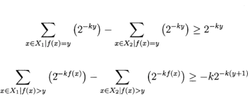
We observe that the first term in 5.11 is necessarily the same for both sets, and can therefore be treated as a constant. Furthermore, we see that the following bounds must exist:

(2-ky) - -ky) > 2-ky (5.12)

xEX1 If(x)=y xGX2 If(x)=y

(2-kf(x)) - (2-kf(x)) > -k2-k(y+l) (5.13)

XEXif(x)>y xEX21f(x)>y

Using 5.11, 5.12, and 5.13, the difference between can be represented as

score(f(-), X1) - score(f(-), X 2) > 2~-ky - k2-k(y+l) (5.14)

Per 5.10, this difference is strictly positive, and therefore

score(f(-), X1) > score(f(-), X2) (5.15)

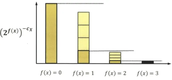
Figure 5-2 depicts this property of the score function.

First we define a function that will help to place parts such that we first maximize the number of parts still available to be placed (i.e., reveal as many new parts as possible). A reasonable function could rank parts first by the number of physical dependencies they satisfy. We can represent this ranking with the score function:

#

(vi) = score(deg- , {vI (vi, vj) E E,}) (5.16) (5.10)

(2f(x)-cx

f(x)

= 0 f(x)= 1 f(x)= 2 f(x)= 3

Figure 5-2: The score function has the property that given two sets, the function will give

a higher score to the set with most values generating the lowest value of

f.

Similarly, we would like to place blocks that are least likely to cause a bottleneck first.

By rating blocks by the number of different ways to reach their children we can place

preference against restricting high-traffic paths. We also would like to tend toward placing parts in harder-to-reach locations first, so we need to define a slightly more complex test

function g(vi) = max(degG,, (vj)) - deg',(vi).

0r (vi) ~ score(g, {vI(v3, vi) E E'}) (5.17)

We also would like to tend toward working in areas far from the easily reachable edge of the system first (i.e., at the end of a hallway). We can use the distance function from Algorithm 3 to measure this:

#r (vi) ~ dist(vi) (5.18)

To combine these two statements we normalize the distance function to between 1 and

1. The score function behaves such that multiplying by a half is the equivalent of redefining

the input function f'(-) = f(.) + 1. In this case doing so would effectively lower the

outdegree of each of a node's children by 1, thus lowering the node's priority. This allows

us to scale

#

by distance without breaking the tiered behavior of the score function. dist(vi ) - 1

kdist (i)-ds(vi) (5.19)

2(max(dist(v)Vv c V, 2) - 1)

Or(vi) = kdist (vi)score(g, {vI(vj, vi) c E'}) (5.20) Finally, in combining these three measures of mass, we need to rescale our masses to allow comparison between

#r

and

#,.

To achieve this we introduce two scaling factors:

#

which rescales the range of in-degrees of nodes in E' to match that of Ep, and 7y which can prioritize reachability or physical dependency as required by the task. The exact tuning of these functions varies depending on the capability and number of each class of robot, and this relationship is left as future work.

max(deg- (vi)) #+ (5.21) max(degG,(V)) Vj E {-1, 0,1} (5.22)

If we define g'(vj) =

#(g(vy)

+ -y), we can introduce those scaling factors to the

reach-ability function by substituting into equation 5.20, which will normalize it to resemble the physical dependency function:

'(vi) = kdist(vi)score(g', {vj|(vj, vi) c E'}) (5.23)

We can now combine equations (5.23), (5.16), and (5.4) to define our combined mass function for use by the controller.

#(Vi) O=c(v1)(#,.(vi) + #,(vi)) (5.24)

5.1

Runtime

Upon the placement of a part, at most c parts will have a change of degree, which in turn means only c2 _{parts have a potential change in mass. This allows constant time for a robot}

Figure 5-3: Part placement while building a solid cube using uniform mass (top) and or-dering (bottom). Note that without the oror-dering algorithm, work in the front occurs first (top middle), making it harder for delivery robots to reach subassemblies in the back. Also note how more of the stacks of blocks in the top right have reached their maximum height, leaving less opportunities for parallelism.

to update all masses after a part has been placed.

5.2

Convergence

Theorem 4 The controller outlined in algorithms 2 and 3 will converge to a complete structure if possible.

Proof 4 Our constraints are described by two DAGs. The mass function we describe here gives positive mass to all vertices with no unplaced parents, which by definition describes and follows a valid topological ordering of both G, and G', and will therefore converge without violating either sets of constraints.

Figure 5-4: The average number of parts with positive mass across time over 50 runs of building a solid cube at the end of a hallway with 5 assembly and 4 delivery robots, with uniform mass on placeable parts (top) and masses calculated using the proposed algorithm (bottom).

Chapter 6

Adaptation in Decentralized Assembly

6.1 Decentralized Scheduling Algorithm in the Presence

of Part Supply Uncertainty

Let us define Av as the part type of part v, and assume all types of the same part are identical and that there are a finite number of part types. Many parts may have the same type, and each assembly requires one or more types of part.

Let the function n(A) represent the number of parts available of type A. We assume that all robots have information about the number and type of robots available, although for our purposes it is sufficient to represent n(A) E {0, 1} as the presence or lack of parts of type

A.

The first modification to our algorithm ensures that a part which we lack is not consid-ered "placeable". We introduce another boolean variable

(6.1)

s(v) = (n(\Av) = 0)

and then redefine our constraint weight to include this variable.

G (v) V (,(V) V G(c)

otherwise

We now introduce two algorithms: one for when a robot receives communication that a

(6.2)

<pc~) = 0 1V)

supply of a certain part type has been extinguished, and another when it receives commu-nication that a part type has been replenished. A diagram demonstrating how a subtree is pruned upon running out of a particular part type can be found in Figure 6-1.

Algorithm 4 Part has been extinguished

1: Receive communication that n(A) = 0

2: E _p - 0

3: El< E,

4: for (vi, vj) E E, : A 3 = Ado 5: E- E U {(vi,v)} 6: _{E +- EP \(v j, vj)}

7: end for 8: E, +- E'

Algorithm 5 Part has been replenished

1: Receive communication that n(A) > 0

2: Ep +- Ep E'\

By making these modifications, we achieve several improvements. First, since a part is

not considered placeable if its supply has run out, an assembly robot will not assign positive demanding mass to those parts. This prevents delivery robots from seeking that part.

Second, by removing the physical dependency of extinguished parts from the parts they depend on, Algorithm 3 will now weight those depended-on parts less. This is desired, because part types that are currently lacking do not provide the robot additional work to perform. Placing physical dependencies does not free up more parts for the assembly robots to place. Doing this ensures that we maintain efficient ordering construction, by pretending that the parts no longer exist in the assembly blueprint.

Note that in this algorithm we did not modify the reachability graph, G,. This is done so that even though we are ignoring the extinguished parts in the dependency graph, we still do not place parts that would prevent placing the extinguished part once the part supply has been replenished.

run out of this part type

temporarily prune subtree

Figure 6-1: When the supply of a part type runs out, the assembly subtree with that part as the root is temporarily pruned. When the part is resupplied, the subtree is added back into the overall assembly tree.

6.1.1

Convergence

Theorem 5 The controller; when modified by algorithms 4 and 5, will converge to a

com-plete structure if possible.

Proof 5 Any time the supply of a part type runs out, the graph will be modified iff parts of

that type remain to be assembled in the structure. Therefore, if the structure is possible to complete the parts will be resupplied. At that time, the controller takes its previous form.

Therefore, if the structure is possible to complete, the modified algorithm will converge to a complete structure.

6.1.2

Runtime

Algorithm 4 requires O(1 V I+

I

I|E ) time to run, since it makes copies of the physical dependencies edges and loops through all nodes in the graph. Algorithm 5 simply makes a copy of the edges, so its runtime is O(1|E,|1).

These two algorithms are only run when a part supply is extinguished or resupplied. Since these two events rely on factors external to the algorithm, it is impossible to com-pletely describe what effects they have on the runtime of the algorithm. However, the mod-ifications that they make to the physical dependency graph do not change the asymptotics

of the underlying algorithm.

6.1.3 Generalization

Note that in the presence of no part supply restrictions, neither algorithm will be utilized during assembly. Therefore this modification can be viewed as a generalized version of the original algorithm that takes part supply into account.

6.2 Decentralized Scheduling Algorithm with Non-Uniform

Assembly Times

Our previous algorithms have assumed that all assembly operations take the same amount of time to accomplish, which is rarely true in practice. For example, one can imagine an assembly where one task is twice as valuable to complete in order to maximize parallelism and efficiency; our prior algorithms would choose the former task to complete first. How-ever, if the first task takes three times as long to complete, then the second task is actually more desirable to complete first. It will make additional work available sooner.

Once we introduce the concept of assembly time, we are no longer interested in the ability of a task completion to make work available; instead, the quantity of interest is a task's ability to make work available divided by the amount of time it takes to complete the task. Mathematically, we introduce this into the algorithm by altering the scoring function. It now takes the form:

score(f(-), X) =[ (2 .(6.3) xEX

where Tx _{represents the amount of time required to complete task x. In the algorithm} the function f (x) represents the number of other nodes that will be affected by completing a task (for example, by fulfilling physical dependencies). By dividing this by the time required to complete that task, we now ensure that we weight assembly tasks according to their actual value to the assembly process.

6.2.1

Convergence

Theorem 6 The controller; when modified by equation 6.3, will converge to a complete

structure if possible.

Proof 6 We have already proved that the original controller will converge to a complete

structure if possible. A part's mass has only a simple linear relationship on the score function. Assuming the time to complete an assembly task, Tx, is a positive number the

sign of the score function is not affected. Therefore the sign of every part's mass is equally unaffected. The order of part placement may change, but a placeable part will not become unplaceable and vice versa. Therefore the structure will converge if originally possible.

6.2.2 Runtime

The addition of an assembly time term to the scoring function does not affect computational complexity or runtime in any significant way.

6.2.3 Generalization

In the case of uniform assembly times such that Tx = T is a constant, the equation 6.3 can be reformatted:

score(f (-), X) = 2- X| (2f(x))C. (6.4)

xEX

As such, the scores and therefore the part weights would be linear scaled version of the

part weights from the original algorithms. As overall scaling does not influence part order,

the assembly order would remain the same. We can therefore view this as a generalized version of the original algorithm that takes assembly time into consideration.

We can also combine this modification with the above part supply algorithm, to make a fully generalized version that takes both assembly time and part supply into consideration.

6.3

Simulations

To test the effectiveness of the part supply modification to our algorithm, we ran it on our

airplane simulation seen in Figure 6-2 using six assembly robots and six delivery robots.

In order to evaluate its effectiveness with respect to part supply, at t=20 the supply of plane

wall panels is extinguished. At t=80 the supply is replenished so that the assembly can

be fully constructed. The simulation was run twenty times: ten times using the original

algorithm, and ten times using the modified part supply algorithm. The results from each

(a) At t = 20 the fuselage panels have run out. Much (b) At t = 80, the fuselage panels are resupplied. of the structure is left to complete. The assembly robots have constructed much of the framework of the fuselage, but were unable to place any fuselage panels in the past 60 timesteps.

(c) The plane has been fully assembled at t = 102 with the resupplied fuselage panels.

Figure 6-2: The plane assembly used in simulation contains a fuselage, two wings, and a tail section, each of which is composed of many individual parts. The parts are color-coded to indicate which robot of the six assembly robots placed each part (e.g., red parts were placed by robot 1, green were placed by robot 2). There are a variety of structural dependencies between parts, making the construction order complex. The plane is shown