A correction function method to solve incompressible fluid flows to high accuracy with immersed geometries

ARCHVEs

A Correction Function Method to Solve

Incompressible Fluid Flows to High Accuracy with

Immersed Geometries

Alexandre N7oll Marques

Submitted to the Department of Aeronautics and Astronautics

in partial fulfillment of the requirements for the degree of

Doctor of Philosophy

at the

MASSACHUSETTS INSTITUTE OF TECHNOLOGY

June 2012

@

Massachusetts Institute of Technology 2012. All rights reserved.

A u th or ...

...

I epartment o

onauticsyd Astronautics

'

e rur

27, 2012

Certified

by...

Rodolfo R. Rosales

Professor of Applied Mathematics

Thesis Supervisor

C ertified by ...

...

...

Jean-Christophe Nave

Professor of Mathematics

Thesis Supervisor

Certified by...

...

Jaime Peraire

Professor of Aeronautics and Astronautics

I

/Thesis

Committee

Certified by...

...

y

'

Steven G. Johnson

Associate Professor of Applied Mathematics

Thesis Committee

A ccepted -by

...

...

Eytan H. Modiano

Chair, Department Committee on Graduate Theses

A Correction Function Method to Solve Incompressible

Fluid Flows to High Accuracy with Immersed Geometries

by

Alexandre Noll Marques

Submitted to the Department of Aeronautics and Astronautics on February 27, 2012, in partial fulfillment of the

requirements for the degree of Doctor of Philosophy

Abstract

Numerical simulations of incompressible viscous flows in realistic configurations are increasingly important in many scientific and engineering fields. In Aeronautics, for instance, relatively cheap numerical computations replace costly hours of wind tunnel investigations in the early design stages of new aircraft. However, standard methods to obtain numerical solutions over complex geometries require sophisticated meshing techniques and intensive human interaction. In contrast, "immersed methods" incor-porate complex boundaries and/or interfaces into regular meshes (Cartesian meshes or simple triangulations). Hence, immersed methods simplify the task of mesh gen-eration and are of great interest in the study of incompressible viscous flows.

The objective of this thesis is to advance current immersed methods by formula-tions that yield highly accurate discretizaformula-tions without compromising computational efficiency. This is achieved by introducing a new type of immersed method, the

cor-rection function method. This new method is based on the concept of a corcor-rection

function that provides smooth extensions of the solution across boundaries and/or interfaces, such that standard (accurate and efficient) discretizations of the governing equations remain valid everywhere in the computational domain. Furthermore, the key concept behind the correction function method is the introduction of the correc-tion funccorrec-tions as solucorrec-tions to partial differential equacorrec-tions, which are defined locally around the immersed boundaries and interfaces. Then, we can solve these equations to any desired order of accuracy, resulting in high accuracy methods.

Specifically, in this thesis the correction function method is implemented to 4 th

order of accuracy in the context of Poisson's equation, the heat equation, and the nonlinear convection advection diffusion in 2D. Then, these techniques are combined

to solve the incompressible Navier-Stokes equations, which govern the dynamics of incompressible viscous flows.

Thesis Supervisor: Rodolfo R. Rosales Title: Professor of Applied Mathematics Thesis Supervisor: Jean-Christophe Nave Title: Professor of Mathematics

Acknowledgments

There are many people that I need to thank for their support and guidance during this challenging journey. First I must thank my advisors, Profs. Ruben Rosales and Jean-Christophe Nave. It was my first time working closely with Mathematicians, and it was decisively one of the most interesting and rewarding experiences I ever had. It was Profs. Nave's vision and enthusiasm that persuaded me to get involved in this particular project and kept me on track to achieve so much. Prof. Rosales' uncanny capacity to identify and simplify the hardest problems was crucial in the development of this work. I am also thankful for their loyalty and commitment when I needed to overcome bureaucratic hurdles so I could focus on science for most of the time.

Furthermore, I thank all MIT professors with whom I had the pleasure to work. In particular, I thank the members of my thesis committee for their constructive criti-cism and recommendations: Profs. Jaime Peraire, Steven Johnson, Youssef Marzouk, and David Darmofal. I also thank the help I received from all the colleagues that I met in this time, specially the Applied Mathematics Fluids Lunch group, David Shirokoff, and Anas Alfaris. In addition, I thank the always prompt assistance from the Department of Aeronautics and Astronautics' staff, specially Jean Sofronas, Beth Marois and Marie Stuppard, and the people at the Department of Mathematics head-quarters.

This work counted with the financial support by Coordenagio de Aperfeigoamento de Pessoal de Nivel Superior (CAPES -Brazil) and the Fulbright Commission through grant BEX 2784/06-8. It was also partially funded by the National Science Foundation through grant DMS-0813648, and the NSERC Discovery program.

Finally, I must thank the unwavering and unconditional love and support I received from my family. I am specially grateful to my loving and caring wife, Nielle Marques, who gave me strength and purpose to move forward, and always made everything possible.

Contents

1 Introduction

1.1 M otivation . . . .

1.2 Literature Review: Immersed Methods . . . .

1.3 Contributions . . . . 1.4 Organization of the thesis . . . .

2 The Correction Function Method 2.1 Definition of the problem . . . . 2.2 The basic idea . . . .

2.3 The correction function and the equati

2.4 A 4th order accurate scheme in 2D . .

2.4.1 Overview . . . .

2.4.2 Standard Stencil . . . . 2.4.3 Definition of Q2 j)...

2.4.4 Solution of the local PDE 2.4.5 Computational Cost . . . . . 2.4.6 Interface Representation . . . 2.4.7 Error analysis . . . . 2.4.8 Computation of gradients . . 2.5 Results . . . . 2.5.1 Example 1 . . . . 2.5.2 Example 2 . . . . 2.5.3 Example 3 . . . . 27 28 . . . . 29 on defining it . . . . 31 . . . . 35 . . . . 35 . . . . 36 . . . . 38 . . . . 42 . . . . 44 . . . . 45 . . . . 4 6 . . . . 4 6 . . . . 4 7 . . . . 48 . . . . 50 . . . . 5 1 7 15 . . . . . 15 . . . . . 18 . . . . . 23 . . . . . 25

2.5.4 Example 4 ... . 55

3 Extensions of the Correction Function Method 59 3.1 Boundary conditions on complex geometries . . . . 60

3.1.1 Overview . . . . 60

3.1.2 The correction function and the equation defining it . . . . 61

3.1.3 Definition of .j..) 63

3.1.4 Solution of the Local PDE . . . . 64

3.1.5 Neumann boundary condition . . . . 66

3.1.6 Results . . . . 67

3.2 Poisson's equation with discontinuous coefficient . . . . 69

3.2.1 Overview . . . . 69

3.2.2 Smooth extensions of the solution . . . . 71

3.2.3 Solution of the Local PDE . . . . 73

3.2.4 Results . . . . 76

4 Alternative Method to Solve the Poisson equation - using boundary integral equations 81 4.1 Solution procedure . . . . 82

4.1.1 Laplace equation . . . . 83

4.1.2 Including a non-homogeneous source . . . . 86

4.1.3 Poisson equation with Piece-wise constant coefficients . . . . . 87

4.1.4 Sum m ary . . . . 90

4.2 R esults . . . . 93

4.2.1 Example 1. Imposing boundary conditions over arbitrarily shaped surfaces . . . . 94

4.2.2 Example 2. Poisson equation with piece-wise constant coefficients 96 5 Dynamic Problems 99 5.1 Heat equation . . . . 100

5.1.1 Overview . . . . 100 8

5.1.2 A compact discretization . . . . 5.1.3 The Correction Function Method . . . . 5.1.4 R esults . . . .

5.2 Convection-Diffusion equation . . . .

5.2.1 Overview . . . . 5.2.2 A compact discretization . . . . 5.2.3 Results . . . .

6 Incompressible Navier-Stokes Equations

6.1 Formulation . . . .

6.2 Numerical Scheme . . . . 6.3 R esults . . . .

6.3.1 Purely periodic boundaries . . . .

6.3.2 Immersed Boundary . . . .

6.3.3 Flow over a cylinder . . . .

7 Conclusion

7.1 Final Remarks. . . . .

7.2 Future work . . . .

A The 9-point stencil for the Poisson equation

B Bicubic interpolation

C Issues affecting the construction of Q''

C.1 Naive Grid-Aligned Stencil-Centered Approach. .

C.2 Compact Grid-Aligned Stencil-Centered Approach. C.3 Free Stencil-Centered Approach . . . .

C.4 Node-Centered Approach . . . . D Ill-posed problem 9 101 103 105 106 106 109 112 115 116 119 123 124 125 129 137 137 139 141 143 145 147 148 149 150 153

List of Figures

1-1 Examples of body-fitted and immersed meshes for the domain between circles of radius 0.1 and 1. . . . . 16

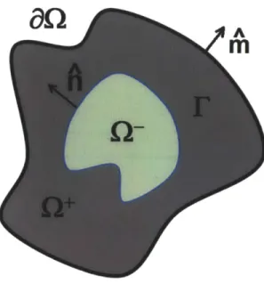
2-1 Example of solution domain Q. The solution is discontinuous across the interface r. . . . . 29

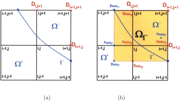
2-2 Example in 1D of a solution with a jump discontinuity. . . . . 30 2-3 (a) The 9-point compact stencil next to the interface F. (b) The set

QO 'j) for this stencil. . . . . 37

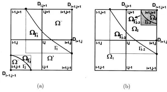
2-4 Configuration where multiple QOf') are needed in the same stencil. (a) Same interface crossing the stencil multiple times. (b) Distinct inter-faces crossing the same stencil. . . . . 41

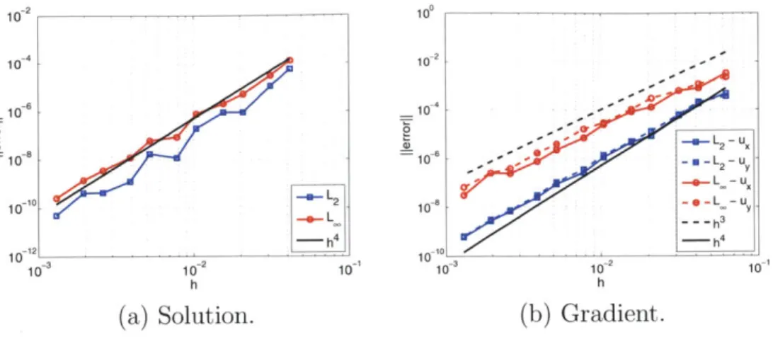
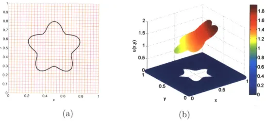
2-5 Example 1. (a) Solution domain embedded in a 33 x 33 Cartesian grid. (b) Solution obtained with a 193 x 193 grid. . . . . 49

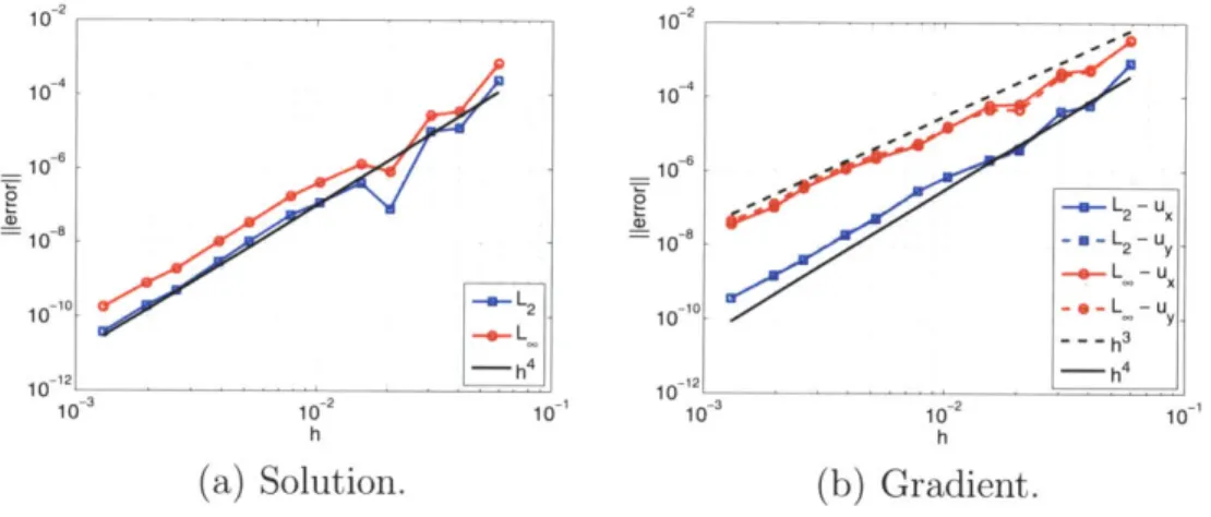
2-6 Example 1. Convergence of the error in the solution and its gradient

in the L2 and L, norms. . . . . 49

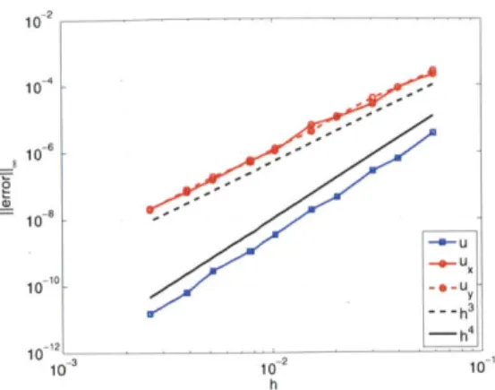
2-7 Example 1. Convergence of the error in the solution and its gradient

evaluated along the interface. . . . . 50 2-8 Example 2. Convergence of the error in the solution and its gradient

in the L2 and L. norms. . . . . 52

2-9 Example 2. Convergence of the error in the solution and its gradient

in the L2 and L, norms. . . . . 52

2-10 Example 2. Convergence of the error in the solution and its gradient evaluated along the interface. . . . . 53

2-11 Example 3. Convergence of the error in the solution and in the L2 and L, norms. . . . .

2-12 Example 3. Convergence of the error in the solution and in the L2 and L, norms. . . . .

2-13 Example 3. Convergence of the error in the solution and

evaluated along the interface. . . . .

2-14 Example 4. Convergence of the error in the solution and in the L2 and L, norms. . . . .

2-15 Example 4. Convergence of the error in the solution and

in the L2 and L, norms. . . . .

2-16 Example 4. Convergence of the error in the solution and

evaluated along the interface. . . . . 3-1 Example of a solution domain with arbitrary shape. . . . 3-2 Steps involved in forming

4Q

...

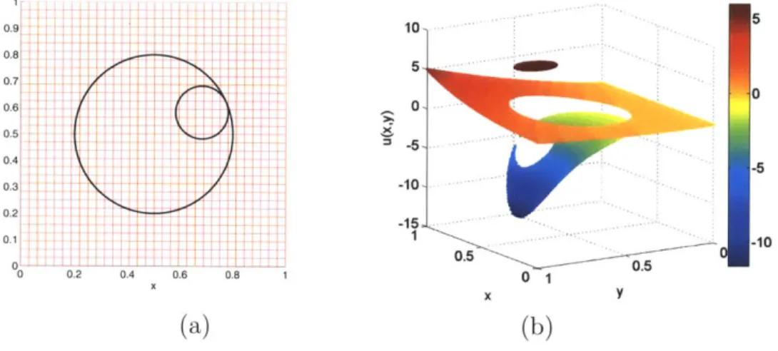
3-3 (a) Solution domain embedded in a 65 x 65 Cartesian grid.

obtained with a 193 x 193 grid. . . . .

3-4 Convergence of the error in the L2 and L. norms...

3-5 Convergence of the error evaluated along the interface. 2-1 Example of solution domain with arbitrary shape. . . . .

3-6 Regions where the extended solutions are defined. This sumes that node (i,

j)

3-7 (a) Solution domain embedded in a 65 x 65 Cartesian grid.

obtained with a 193 x 193 grid. . . . . ...

3-8 Convergence of the error in the L2 and L, norms....

3-9 Convergence of the error along the interface. . . . .. 4-1 Rectangular domain B that involves Q. . . . . 4-2 (a) Solution domain embedded in a 33 x 33 Cartesian Grid.

obtained with a 193 x 193 grid. . . . .

4-3 Error convergence in L2 and L, norms .. . . . .

its gradient its gradient its gradient its gradient its gradient its gradient (b) Solution example as-(b) Solution (b) Solution 12 85 95 96

4-4 (a) Solution domain embedded in a 33 x 33 Cartesian Grid. (b) Solution

obtained with a 193 x 193 grid. . . . . 98

4-5 Error convergence in L2 and L. norms. . . . . 98

3-1 Example of solution domain with arbitrary shape. . . . . 100

5-1 (a) Solution domain embedded in a 65 x 65 Cartesian grid. (b) Con-vergence of the error in the L2 and L, norms. . . . . 106

5-2 Solution at different times. . . . . 106

5-3 Convergence of the error along the boundary. . . . . 107

5-4 Solution domain discretized with a 65 x 65 Cartesian grid. The internal boundary is immersed in the grid. . . . . 113

5-5 Plot of the u component of the solution at different times. . . . . 113

5-6 Plot of the v component of the solution at different different in time. 113 5-7 Convergence of the error in the L, and L2 norms. . . . . 114

5-8 Convergence of the error along the boundary. . . . . 114

6-1 Solution at t = 10 for Re = 1. . . . . 125

6-2

L.

6-3 Convergence of the error in the L. norm. . . . . 126

6-4 Solution domain with the boundary immersed in a 96 x 96 Cartesian grid. . . . .. . .. . . . . . . 127

6-5 Solution at t = 1 for Re = 1. . . . . 127

6-6 (a) Variation of the L, norm of the divergence of the velocity over time. (b) Convergence of the error in the L. norm. . . . . 128

6-7 Convergence of the error along the boundary. . . . . 128

6-8 One period of the infinite array of cylinders. The boundary is immersed in a 268 x 128 Cartesian grid. . . . . 130

6-9 Solution at t = 6 for Re = 1. Speed denotes s = vu2 + 2. . . . . 131

6-10 Streamlines of the flow around the cylinder at t = 6, with Re = 1. . . 131

6-11 (a) Variation of the L, norm of the divergence of velocity over time. (b) Nondimensional forces acting over the cylinder: drag and lift. . . 132

6-12 Solution at t = 6 for Re = 30. Speed denotes s = / 2

+

. . . . . . 132 6-13 Streamlines of the flow around the cylinder with Re = 10. . . . . 133

6-14 (a) Variation of the L, norm of the divergence of velocity over time.

(b) Nondimensional forces acting over the cylinder: drag and lift. . . 133 6-15 Solution at t = 30 for Re = 20. Speed denotes s = /u2+ v2. . . . . . 134

6-16 Solution at t = 60 for Re = 20. Speed denotes s =

V2+

6-17 Streamlines of the flow around the cylinder with Re = 20. . . . . 135 6-18 Streamlines showing vortex shedding behind cylinder for t > 50. . . . 136 6-19 (a) Variation of the L, norm of the divergence of velocity over time.

(b) Nondimensional forces acting over the cylinder: drag and lift. . . 136

3-1 Q~j as defined by the naive grid-aligned stencil-centered approach. . 147

3-2 Qbj as defined by the compact grid-aligned stencil-centered approach. 148

3-3 Q2j as defined by the free stencil-centered approach. . . . . 150

3-4 Q5j as defined by the node-centered approach. . . . . 151

Chapter 1

Introduction

1.1

Motivation

Many applications in science and engineering involve the dynamics of incompress-ible viscous flows. From mixtures of immiscincompress-ible fluids [1, 2], to motion of micro-organisms [3], to flight of insects [4,5], to the flow of blood in the heart [6]. In Aero-nautics, the airflow over low-speed aircrafts can often be idealized as incompressible. Such is the case with many of the unmanned air vehicles (UAVs) in production today (e.g. USAF's MQ-1B Predator cruises at Mach 0.11 [7]). Moreover, even though many of the characteristics of the airflow over these vehicles can be estimated with simplified inviscid models, there are important features that can only be accurately determined by including viscous effects, such as drag force and flow separation.

The advances in computational power and memory over the last decades have made it possible to study increasingly realistic and complex flow configurations with numerical methods. However, an accurate representation of the complex geometries involved in many applications demands sophisticated meshing techniques, such as multi-block meshes [8,9], octree decomposition [10], automatic triangulations [11], and hybrid methods [12,13] (for a thorough review, see [14]). Although these tech-niques constitute very powerful tools for mesh generation, the task of creating ade-quate meshes for complex geometries still requires a considerable amount of human interaction. This issue is even more complicated if the boundaries or the interfaces

are moving in unsteady simulations. Since regular solvers require a body-fitted mesh (see figure 1-1(a)), one needs an algorithm to adapt the mesh to the motion of the boundary at every time step. A common practice is to deform the original mesh to account for the motion of the boundary [15-17]. In some situations, it is possible to construct a smooth mapping between the deformed mesh and a reference mesh. In this case, one can use arbitrary Lagrangian-Eulerian (ALE) methods to account for the mesh deformation in a accurate fashion [16]. However, in general situations the process of mesh deformation can be costly and adds errors to the solution. More-over, in extreme cases (e.g. large deformations, interfaces merging/splitting) complete remeshing may be necessary.

crl _o 0.2 _. -0.2 ... 0 .2 i -0.4... _-0.2 -0.46 ....-. -0.8-r -1 05 0 0. 1 0. 1 X X

(a) Body-fitted mesh. (b) Immersed mesh.

Figure 1-1: Examples of body-fitted and immersed meshes for the domain between circles of radius 0.1 and 1.

To avoid the complications related to creating quality body-fitted meshes and adapting the mesh to moving boundaries, a family of "immersed methods" for in-compressible viscous flows has arisen over the last four decades. In these methods, one does not need to fit the mesh to the boundary or interface (see figure 1-1(b)): boundaries and/or interfaces are immersed into regular meshes (Cartesian meshes or simple triangulations), and the methods automatically adapt the discretization to the boundary or interface conditions. A thorough literature review of this class of methods is presented in the next section.

Despite recent advances, many of these methods are at most second order accurate

- with a few exceptions. Moreover, in general, either immersed methods do not offer clear extensions to higher orders of accuracy, or the extensions are excessively convoluted and inefficient. The objective of this thesis is to contribute to the theory of immersed methods by introducing a general formulation that allows the systematic creation of numerical schemes with high order accuracy. Hence, this thesis is focused on a completely new concept, rather than simply on extending the already existing immersed methods.

The method presented in this thesis is based on the construction of smooth ex-tensions of the solution across boundaries and interfaces. These exex-tensions are then used to define correction functions, which can be used to "complete" standard dis-cretizations of the equations. Hence the name correction function method (CFM). The key concept behind the CFM is characterizing the correction functions as solu-tions to partial differential equasolu-tions defined locally in the vicinity of the boundaries and interfaces. The idea of extending the solution is not new, but defining these extensions as the solution to PDEs is an entirely original concept. Furthermore, in principle one can devise schemes to solve these local PDEs to any desired order of accuracy. Therefore, this concept is the main feature of the CFM that allows us to obtain high order of accuracy.

The incompressible viscous flows of interest in this thesis are described by the incompressible Navier-Stokes equations (INSE). A common practice to solve these equations is reformulate the problem in terms of a nonlinear convection-diffusion equation for the velocity distribution, and a Poisson equation for the pressure distri-bution [18-26]. The core contridistri-butions of this thesis are

(i) A new and highly accurate CFM to solve the Poisson equation with immersed boundaries.

(ii) A new and highly accurate CFM to solve the nonlinear convection-diffusion equation with immersed boundaries.

(iii) The integration of these methods to solve the incompressible Navier-Stokes equa-tions to high order of accuracy with immersed boundaries.

1.2

Literature Review: Immersed Methods

Immersed methods were originally conceived to solve problems with interfaces (or infinitely thin membranes) dividing multiphase flows, and later extended to deal with complex boundaries in a immersed fashion. Hence, much of the development in this area happened around interface problems. Two important aspects must be considered when using immersed methods: (a) the representation (and tracking) of the interface, and (b) the discretization of the governing equations in the vicinity of the interface. The latter ultimately characterizes the different methods, but the development of both aspects is intertwined.

There are two classes of methods used to represent the interface: explicit and implicit. Explicit methods are based on introducing fictitious particles that represent the location of the interface. The advantage of explicit representations is that one can follow the interface by simply tracking the individual particles that move according to simple kinematics. Probably the first explicit method was the marker and cell

(MAC) method introduced by Harlow and Welch [27-29]. This method is aimed

at flows with a free surface. Basically, fictitious markers are introduced within the fluid and the position of the outermost markers characterize the location of the free surface. Another explicit approach is to place particles along the interface itself

[30-32]. The location of the neighboring particles is used to produce local interpolations

(e.g. splines), which are then applied to compute geometric information - such as curvature and normal directions. Although this approach can be quite accurate, it requires special treatment when the interface undergoes either large deformations or topological changes - such as mergers or splits. This issue can be particularly

challenging in 3D [32].

On the other hand, in an implicit representation the location of the interface is extracted from some function that is defined everywhere in the regular computational grid. An early implicit representation was obtained by extending the MAC method

into the volume-of-fluid (VOF) method [2, 33, 34]. In the VOF, instead of using

markers, one registers the partial volume occupied by the fluid in each cell of the grid.

This approach is more efficient than MAC since it considerably decreases the number of degrees of freedom necessary to track the free surface, but it does not result in better accuracy. A more popular approach to represent the interface implicitly is the level set (LS) method introduced by Osher and Sethian [35-39]. In the LS method, the interface is given by the zero level of a function defined everywhere in the domain. The basis of the LS method, however, is the effective and efficient algorithm that is used to advance the interface by advecting the LS function with the local fluid velocity. The success of the LS method gave rise to a vast literature that covers a wide range of applications other than flow problems [40,41]. In particular, in this thesis the gradient-augmented level set (GA-LS) method [42] was adopted. With this extension of the LS method, one can obtain highly accurate representations of the interface, and other geometric information, with the additional advantage that this method uses only local grid information.

As mentioned before, a common practice to solve the incompressible Navier-Stokes equations (INSE) is to reformulate the problem in terms of a nonlinear convection-diffusion equation and a Poisson equation. When the solution is known to be smooth, it is easy to obtain highly accurate discretizations to these equations on a regular grid. Furthermore, these discretizations usually yield symmetric and banded linear systems, which can be inverted efficiently [43]. On the other hand, when singularities occur (e.g. discontinuities) across internal interfaces, some of the regular discretization stencils will straddle the interface, which renders the whole procedure invalid.

Several strategies have been proposed to tackle this issue. Peskin [30] introduced the immersed boundary method (IBM) [6, 30, 44-47], in which the discontinuities are re-interpreted as additional (singular) force terms concentrated on the interface. These singular terms are then "regularized" and appropriately spread out over the reg-ular grid - in a "thin" band enclosing the interface. This approach is very appealing since the discretization of the flow equations is not affected, only the right-hand-side (RHS). The result, however, is a first order scheme that smears discontinuities. Gold-stein [48] presents an extension of the IBM where linear control theory is used to compute the singular forces needed to impose the no-slip condition on a boundary

of the domain. A more direct method to determine the singular forces for this prob-lem was later introduced by Fadlun et al. [49]. A recent review of the IBM and its applications was presented in [47].

In order to avoid the smearing of the interface information, LeVeque and Li [50] developed the immersed interface method (IIM) [50-54], which is a methodology to modify the discretization stencils, taking into consideration the discontinuities at their actual locations. The IIM guarantees second order accuracy and sharp discontinuities, but at the cost of added discretization complexity and loss of symmetry. The IIM was also extended to treat no-slip boundary conditions by adding singular forces along the boundary in the work of Le et al. [55]. This extension preserves the second order accuracy of the IIM. Recently, Zhong [56] introduced a new version of the IIM where the modified discretization stencils are obtained by matching polynomials on both sides of the interface. The result is a high order method based on wide dimension-by-dimension stencils.

The new method advanced in this thesis builds on some ideas introduced by the ghost fluid method (GFM) [57-62]. The GFM is based on defining both actual and "ghost" fluid variables at every grid node that lies in a narrow band enclosing the interface. The ghost variables work as extensions of the actual variables across the interface - the solution on each side of the interface is assumed to have a smooth extension into the other side. After the ghost values are computed, one can apply standard discretizations everywhere in the domain. Moreover, in most GFM versions the ghost values are written as the actual values, plus corrections that are inde-pendent on the underlying solution to the problem. Hence, the corrections can be pre-computed, and moved into the source term for the equation. In this fashion, the

GFM yields the same linear system as the one produced by the problem without

an interface, except for changes in the RHS only. Thus, this linear system can be inverted just as efficiently as in problems with smooth solutions. The key difficulty in the GFM is the calculation of the correction terms, since the overall accuracy of the scheme depends heavily on the quality of the assigned ghost values. In [57-61] the authors develop first order accurate approaches to deal with discontinuities.

It is relevant to note other methods developed to solve boundary problems in a immersed fashion. Mayo [31] introduced a method to solve the Laplace equation in which one first solves a boundary integral equation to obtain "jump conditions" over the boundary. After these jump conditions are known, one can solve the Laplace equation using finite differences. The jump conditions are used to create corrections to the RHS of the discretized equation, similarly to the GFM (even though Mayo's method preceded the GFM). Moreover, since the solution to the integral equation can also yield jump conditions in derivatives of the solution, this method can be used to create corrections to high order accuracy. Mayo [31,63] shows second and fourth order results. Extensions of Mayo's method to the Poisson equation are presented in [63,64]. In §4 similar ideas are used to solve Poisson equations in general configurations.

Johansen and Colella [65] introduced a second order accurate finite volume dis-cretization of the incompressible Navier-Stokes equations (INSE). This method is based on building second order approximations to the fluxes on the edges of partial cells (cells cut by the boundary) based on quadratic interpolations in the direction normal to the boundary. The result is a second order accurate method that yields non-symmetric linear systems. Jomaa and Macaskill [661 use a similar concept to obtain a finite-difference discretization of the Poisson equation with immersed boundary. In their work, however, Jomaa and Macaskill [66] show that stencil modifications based on dimension-by-dimension linear interpolations suffice to yield second order accuracy, resulting in a symmetric discretization. In addition, Linnick and Fasel [67] were able to build a fourth order accurate method to solve the Navier-Stokes equa-tions in stream function-vorticity formulation with complex boundaries in a immersed fashion. This method introduces modifications to a fourth order accurate compact finite-difference discretization of the equations using concepts similar to the IIM.

Similar methods were also developed for situations where Dirichlet-type condi-tions are applied to an internal interface. Such is the case with Stefan problems that describe the solidification/liquefaction of pure substances, including unstable solidifi-cation that leads to dendritic crystal growth [37,68]. Udaykumar et al. [32] introduced a method to solve the full INSE to second order of accuracy for problems with phase

transformation. In this method, the INSE are discretized using regular second-order finite-difference stencils, except for the vicinity of the interface, where a first order and non-symmetric discretization is devised to enforce the appropriate interface con-ditions. Gibou et al. [69] introduced a formulation similar to the GFM to discretize the Poisson equation to solve the Stefan problem. However, in this work, the final discretization is second order accurate and symmetric. Later, Gibou and Fedkiw [70] developed a fourth order accurate version of this discretization, at the cost of giving up symmetry. More recently, the same problem has also been solved, to second order of accuracy, in non-graded adaptive Cartesian grids by Chen et al. [71].

The finite element community has also made significant progress in incorporating the IIM and similar techniques to solve the Poisson equation using immersed grids. Finite element formulations have the advantage that they usually produce symmet-ric discretizations of self-adjoint operators, and that they are (in principle) easily extendible to high orders of accuracy and to higher dimensions. However, they also require (at least for the current approaches for immersed problems) "special" elements and/or integrations over partial elements. Hence, even though most of these methods yield symmetric discretizations, most applications are still restricted to second order accuracy in 2D.

One popular finite element method to solve elliptic problems with immersed in-terfaces is the penalty method [72-74], where interface conditions are added with penalization parameters to the weak formulation of the problem. Mo~s et al. [75] in-troduced the extended finite element method (X-FEM) in the context of modelling the growth of cracks. In essence, the X-FEM uses an enriched basis to represent the so-lution adjacent to cracks, incorporating appropriate enrichment functions that model displacement discontinuities introduced by the cracks. Other more general immersed finite-element formulations include the finite-element embedded interface method by Dolbow and Harari [76], the virtual node method by Bedrossian et al. [77], and ex-tensions of the IIM [54,78-80], and the exact subgrid interface correction method by Huh and Sethian [81].

In the context of the finite volume method, the cut-cell method [82-84] became a 22

standard approach in fluid flow applications with immersed boundaries. This method was later adapted to finite elements [85], and recently incorporate in a DG discretiza-tion of the compressible Navier-Stokes equadiscretiza-tions [86].

1.3

Contributions

In this thesis a new method is presented - the correction function method - to solve incompressible viscous flows to high order of accuracy. This new method is of the "immersed" kind, in which the boundaries and/or interfaces are immersed into un-derlying regular meshes.

One key step needed to solve the incompressible Navier-Stokes equations (INSE) is the solution of the Poisson equation. Hence, one of the core contributions of this thesis is the development of a correction function method that can be used to solve the Poisson equation to high order of accuracy using immersed grids. Furthermore, within the context of the Poisson equation there is a number of configurations of interest to fluid flow applications. In this thesis the Poisson equation is solved in the context of (i) discontinuous solutions across internal interface, (ii) discontinuous coefficients, and (iii) immersed boundaries. The method used to solve situation (i) is called the "original" correction function method, since it serves as the foundation for the correction function method used in all other applications discussed in this thesis. This original version of the CFM was published in the Journal of Computational

Physics [87].

Other contribution of the thesis is the extension of the CFM to dynamic problems related to fluid flow phenomena. In particular, the thesis includes the solution of the heat equation and of the nonlinear convection-diffusion equation with immersed boundaries. This contribution involves the creation of a concept of extended solutions and correction functions that stretches over time and is valid for dynamic equations. In addition, this extension is crucial to fluid flow applications because we need to solve a nonlinear convection-diffusion equation to obtain the velocity distribution in incompressible viscous flows.

The final contribution of the thesis is putting the techniques mentioned above together to create a numerical solver for the INSE. This numerical solver is capable of obtaining solutions to high order of accuracy with boundaries that are immersed into regular Cartesian grids. This step also involves writing the INSE in a formulation that is suitable for an accurate CFM discretization.

In summary, the contributions of this thesis can be separated into three categories:

1. Poisson equation: development of a new family of immersed schemes - the

cor-rection function method (CFM). These schemes yield highly accurate

discretiza-tions that can be efficiently inverted for the following problems.

" Constant coefficients Poisson equation with jump discontinuities across an

internal interface.

" Discontinuous coefficient Poisson equation with jump discontinuities across

an internal interface.

" Poisson equation with "immersed boundaries."

2. Dynamic problems: extension of the CFM to dynamic equations of interest in fluid flow applications. In particular, this thesis includes

" the heat equation.

" the nonlinear convection-diffusion equation.

3. Incompressible flow solver: use of the CFM to solve the incompressible

Navier-Stokes equations. This step involves splitting these equations into a nonlinear convection-diffusion equation for the velocity distribuion, and a Poisson equation for the pressure distribution. Then, the techniques developed in items 1 and 2 are used to create a numerical scheme that can solve incompressible viscous flows to high order of accuracy with immersed boundaries.

1.4

Organization of the thesis

The remainder of this thesis is organized as follows. In §2 the "original" version of the correction function method is introduced. This version is designed to solve the constant coefficients Poisson equation, with jump discontinuities (with some restric-tions) imposed across an interface internal to the solution domain. In this chapter, the basic concepts and machinery that are behind all other versions of the CFM are discussed in detail.

Then in §3 the original CFM is extended to solve (i) the Poisson equation with an immersed boundary, and (ii) the discontinuous coefficient Poisson equation. The biggest difficulty in these cases is that the PDE that defines the correction function is coupled to the underlying solution of the Poisson equation. The approach used to handle this coupling between the equations is discussed in §3. Next, §4 presents an alternative approach to solve these same problems. In this alternative approach, one first solves a boundary integral equation to obtain new "jump conditions." After this step, a general Poisson equation can be rewritten as an equivalent constant coefficients Poisson equation with discontinuous solution. Then this equivalent problem can be solved with the original CFM.

Chapter §5 is dedicated to the solution of the heat equation and of the nonlin-ear convection-diffusion equation, both with immersed boundaries. In this chapter the concept of a correction function is extended to the context of dynamic prob-lems. Then, in §6 the techniques discussed in §3 and §5 are combined to solve the incompressible Navier-Stokes equations. Finally, in §7 are the concluding remarks, including a summary the most important features of the methods described in the thesis, and a list of open areas for possible future work.

Chapter 2

The Correction Function Method

In this chapter the original version of the correction function method (CFM) [871 is introduced. This original version was designed to solve the constant coefficients Pois-son equation in situations where the solution is discontinuous across some arbitrary interface. A formal definition of this problem is presented in §2.1. Extensions of the CFM to solve the Poisson equation under more general circumstances are discussed

in in §3 and §4.

The basic idea behind the correction function method is to create smooth exten-sions of the solution from both sides of the discontinuity into the other side. Once these extensions are known, one can use a standard discretization of the Poisson equation everywhere in the solution domain. This idea, and its relationship to the ghost fluid method, are explained in detail in §2.2. Furthermore, these extensions can be used to define a correction function, which is characterized as the solution to a partial differential equation, as shown in §2.3. Next, in §2.4 this concept is applied to build a 4th order accurate scheme in 2D. In addition, the domain of definition of the correction function deserves special attention, so appendix C is dedicated to explaining some details that are left out of §2.4. Finally, in

§

accuracy of the 2D scheme are demonstrated by applying it to numerical examples.

2.1

Definition of the problem

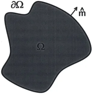
The original version of the CFM was designed to solve the constant coefficients Poisson equation in a domain Q in which the solution is discontinuous across a co-dimension 1 interface IF. This interface divides the domain into the subdomains Q+ and Q-, as illustrated in figure 2-1. The notation

(.)+

conditions are imposed on the outer boundary 8Q. Thus the problem to be solved is

AUs) = f V)

for Y E Q,

(2.la)

[u] = a(g) for Y E F, (2.1b)

[un] =

b(Y)

Y

IF,

u(9) = g(g) for Y E a, (2.1d)

where

[. ()

G_()-

(2.2a)

denotes jumps across an internal interface. Throughout this chapter, z = (x1, x2, .-. ) E

R' is the spatial vector (where v = 2, or v = 3), and A is the Laplacian operator

defined by

A (2.3)

Furthermore,

U"

iU

denotes the derivative of u in the direction of ft, the unit vector normal to the interface

F pointing towards Q+ (see figure 2-1).

Moreover, note that this version of the CFM is focused on the discretization of the problem in the vicinity of the interface only. Thus, the method is compatible with

Figure 2-1: Example of solution domain Q. The solution is discontinuous across the

interface F.

any set of boundary conditions on &Q, not just Dirichlet, as long as these boundary

conditions are properly enforced. In the examples included in this chapter, OQ is

rectangular. Extensions of the CFM to arbitrarily shaped boundaries are discussed

in §3 and §4.

2.2

The basic idea

The correction function method is based on the concept of a correction function. This

concept is a generalization of the ideas of the ghost fluid method (GFM). In essence,

one starts with a standard finite-differences discretization of the Laplace operator

(e.g. 5-point or 9-point stencil). Whenever the discretization stencil straddles the

interface F, the corrections are used on the right-hand-side (RHS) of the discretized

equation to incorporate the jump conditions. As a consequence, the linear system

that results from the finite-differences discretization is not altered, only the RHS.

Thus, this linear system can be inverted as efficiently as in the case of a solution

without discontinuities.

a

b

.

i-1

]

Q

+1

Figure 2-2: Example in 1D of a solution with a jump discontinuity.

dimensional Poisson equation: uX (x)

f(x),

for

Then, assume that u

is discontinuous at

with Q+

X :

< x

and Q

The standard

order centered differences discretization of the equation is

+ ~ -1 - 2 +1 _(2.5)

uX, ~" _h2

where h

xi+1

-

xi is the grid spacing - see figure 2-2. However, in the situation

depicted in figure 2-2, x <

< xi+1. Thus, at xi+

only u;+

is defined, not u+1

A1,

(2.5)

1 - 2+ (u+1

+

(26)

uX~ , ~ h2(26

Note that, if the correction Di+

is independent on the solution u, then it can be

moved to the RHS of the equation, and absorbed into

f.

That is

ut_ - 2nit

ut1i

+

(2.7)

h2 h2.(27

With this procedure, the problem with discontinuities can be solved with the same

discretization used to solve the continuous problem. Hence, the resulting linear system

can be inverted using the same well established and efficient techniques available for

D.-the continuous Poisson equation [43].

Remark 2.1. The final accuracy of the discretization depends on the quality of D.

Liu, Fedkiw, and Kang [59] estimate D using a dimension-by-dimension linear ex-trapolation of the interface jump conditions - i.e. the functions a and b in (2.1). The

result is a first order approximation for D. The CFM is based on generalizing the idea of the correction term to that of a correction function, which can be characterized as the solution to a partial differential equation. Then, high accuracy representations of

D follow from solving this equation to high order accuracy, without the complications

introduced by dimension-by-dimension Taylor expansions. 4

Remark 2.2. An additional advantage of the correction function approach is that

D can be evaluated at any point near the interface F. Hence, the CFM can be used

with any finite differences discretization of the Poisson equation, without regard to the particulars of the stencil (as would be the case with any approach based on Taylor expansions).

2.3

The correction function and the equation

defin-ing it

As mentioned above, the idea of the CFM is to generalize the concept of correction terms defined at certain grid nodes to that of a correction function, and then to find a partial differential equation (PDE) - with appropriate boundary conditions - that uniquely characterizes the correction function. Then, at least in principle, one can design algorithms to solve this PDE to obtain the correction

function to any desired

Consider a small region Qr that encloses the interface r, defined as the set of all the points within some distance R of r. The value R is of the order of the grid size h. As explained below, R must be as small as possible. On the other hand, Qr has to include all the points where the CFM requires corrections to be computed,

which means that R depends on the discretization stencil being used'. In addition, algorithmic considerations (to be seen later) may force R to be slightly larger than what is needed to include the discretization stencil.

Next, assume that both u+ and u- can be extrapolated, so that they are valid everywhere within Qr and satisfy the following Poisson equations.

Au+(V) =

f+(+)

Au-(V) =

f-(V)

where

f+

f-

f

The correction function is then defined by D(Y) = u+

(i)

AD(Y) =

f+(Y)

Qr,

D(Y) = a(Y) for Y E I, (2.9b) Dn(Y) = b(Y) for Y E F. (2.9c)

This PDE defines the correction function as the solution to a set of equations, with some provisos - see remark 2.4 below. Note that:

1. If the source term is continuous across Q, then fD = 0.

2. Equation (2.9c) imposes the true jump condition in the normal direction, whereas some versions of the GFM rely on a dimension-by-dimension approximation of this condition [59].

Remark 2.3. The smoothness requirement on

f+

f

'In particular, the 9-point stencil is used in this thesis, so 1R cannot be smaller than Vrh.

if D is at least C4 . Hence, in this case, fD = +

f-

46

Remark 2.4. Equation (2.9) is an elliptic Cauchy problem. In general, such

prob-lems are ill-posed. However, (2.9) is well posed in the special context of a numerical approximation where

(a) There is a frequency cut-off in (i) the data a = a(Y) and b = b(z!), and (ii) the

description of the curve IF.

(b) The solution is needed only a small distance away from the interface IF, where

this distance vanishes simultaneously with the inverse of the cut-off frequency mentioned in point(a).

Because of these conditions, the arbitrarily large growth rate for arbitrarily small perturbations, which is responsible for the ill-posedness of the Cauchy problem, does not occur.

The reason the arbitrarily large growth does not occur is as follows. Consider a perturbation to the solution to Poisson equation along some straight line. Assume a sinusoidal perturbation with wave number 0 < k < o. Then the perturbation grows as e2,skd, where d is the distance from the line. However, by construction, in the present case conditions (a) and (b) guarantee that kd is bounded.

4

Remark 2.5. A number characterizing how well posed the discretized version of (2.9) is can be defined as:

a = _{largest growth rate possible,}

where growth is defined relative to the size of a perturbation to the solution on the interface. This number is determined by R (the "radius" of Gr), as the following calculation shows. First, there is no loss of generality in assuming that the interface is flat, provided that the numerical grid is fine enough to resolve F. In this case, consider an orthogonal coordinate system y on F, and let d be the signed distance to F (say, d < 0 in Q-). Expanding the perturbations in Fourier modes along the

interface, the typical mode has the form

= e2ik-±2,rkd

where k is the Fourier wave vector, and k =

Iki.

maximum growth rate is

a ~e7rR/h.

Moreover, as noted in item (b) of remark 2.4, the size of 1? is proportional to h.

Hence, the maximum growth rate is always bounded. 4

Remark 2.6. Clearly, a is intimately related to the condition number for the

dis-cretized problem - see §2.4. In fact, at leading order, the two numbers should be (roughly) proportional to each other - with a proportionality constant that depends on the details of the discretization. For the discretization used described in §2.4, -Vh <

1? <

Remark 2.7. Equation (2.9) depends only on the known inputs of the problem:

f+,

f-,

Remark 2.8. When developing an algorithm for a linear Cauchy problem, such as (2.9), the two key requirements are consistency and stability. In particular, when

the solution depends on the "initial conditions" globally, stability (typically) imposes stringent constraints on the "time" step for any local (explicit) scheme. This would seem to suggest that, in order to solve (2.9), a "global" (involving the whole domain

Qr) method will be needed. This, however, is not true: because the solution of (2.9)

is needed for one "time" step only - i.e. within an 0(h) distance from 1, stability is

not relevant. Hence, consistency is enough, and a fully local scheme is possible. In the algorithm described in

§2.4

contained in each patch is of the same order as the diagonal length of the patch. This result is in line with the calculation in remark 2.5: we want to keep the "wavelength" (along r) of the perturbations introduced by the discretization as long as possible. In particular, this should then minimize the condition number for the local problems

-see remark 2.6.

4

2.4

A

order accurate scheme in 2D

2.4.1

Overview

In this section the general ideas presented in §2.3 are used to develop a specific example of a 4 th order accurate scheme in 2D. The key points of this scheme are

(a) The Poisson equation is discretized using a compact 9-point stencil - see appendix

A. Compactness is important since it is directly related to the size of R, which

has an impact on the problem's conditioning - see remarks 2.4 to 2.6.

(b) The interface F is represented using the gradient-augmented level set method

-see [42]. This method guarantees a local ₄th order representation of the interface, as required to keep the overall accuracy of the scheme.

(c) The domain Qr is sub-divided into small rectangular regions dubbed O-'i. Each of these regions is associated with a point in the grid at which the standard discretization of the Poisson equation involves a stencil that straddles the interface

17. Furthermore, '(ij) encloses a portion of F, and all the nodes where D is needed to complete the discretization of the Poisson equation at the (i, j)-th stencil. (d) Within each O('j, the correction function D is approximated using a bicubic

interpolation. This approximation guarantees local 4th order accuracy with only

12 interpolation parameters 2

(e) In each O('j, the PDE (2.9) is solved in a least squares sense. Namely: First we define an appropriate positive quadratic integral quantity J, equation (2.14), for which the solution is a minimum (actually, zero). Next, we substitute the bicubic approximation for the solution into J, and the integrals are discretized using Gaussian quadrature. Finally, we find the bicubic parameters by minimizing the discretized J.

Remark 2.9. Solving the PDE in a least squares sense is crucial, since an

algo-rithm is needed that can deal with the myriad ways in which the interface F can be placed relative to the fixed rectangular grid used to discretize the Poisson equation.

This approach provides a scheme that (i) is robust with respect to the details of the interface geometry, (ii) has a formulation that is (essentially) dimension independent

- there are no fundamental changes from 2D to 3D, and (iii) has a clear theoretical underpinning that allows extensions to higher orders, or to other discretizations of

the Poisson equation. ₄

2.4.2

Standard Stencil

In this thesis we use the standard ₄th order accurate 9-point discretization of the Poisson equation (see appendix A):

LoUi,3 + ±(h + hy)&22byy&uu = fij + - (f ), + h (y),), (2.10) where L5 is the 2nd order 5-point discretization of Laplace's operator - see equation

(A.1).

In the absence of discontinuities, expression (2.10) provides a compact 4th order

accurate representation of the Poisson equation. On the other hand, in the vicinity 2

The standard bicubic interpolation requires 16 interpolation parameters. However, in the the-sis we use the version introduced in [42], which needs only 12 parameters. For more details, see appendix B.

of the interface F we need to compute correction terms to complete the

discretiza-tion, as described in detail next. To understand how the correction terms affect the

discretization, consider the situation depicted in figure 2-3(a). In this case, the node

(i, j) lies in Q+ while the nodes (i+1, j), (i+1,

j

+1), and (i,

j+1)

are in Q~. Hence,

to be able to use the discretization (2.10), we need to compute Di+1,,, Di+

, +

, and

Di,j+1-(a)

Figure 2-3: (a) The 9-point compact stencil next to

for this stencil.

After having solved for D where necessary (see

terms modify the RHS on (2.10) as follows.

(b)

the interface 1.

(b)

§2.4.3 and §2.4.4), the correction

L u,j +

2(h2 + h

nij = fij

+

2(h2

+

h2 (fyy),j)

Ci,,

(2.11)

Here the Cjj are the CFM correction terms needed to complete the stencil across the

discontinuity at F. In the particular case illustrated in figure 2-3(a),

(2.12)

(h

+ h

(h

+ h

1-Csy=6

(hxhy)2

(hx

1

(h2

+

Or ""V~