Correlation detection using stored signals

DECLASSIrgN

CLAS

SJFAE

This material contains information affecting the

fnationasl flefo-

4.pof

1Tnitd

n tqtfRf witln +baw

me .1: nin- o* .e E ;niz\nagb Laws, Tit.e 18, lU. S. C.,

sections 793 i,'d 7)4. The transmission or the revelation f its contenkis

in

any mrrinner to an

unauthorized person is prohibited by

law.

CORRELATION ETECTION USING STORED SIGNALS

by

Clatssflcation

Changed

p·v B

Nr

1

I."!J

t4

4IFIED

PAUL EIOT GREEN, JR.

D

r

/

L t

..

W8 Date

A.B., University

of

North Carolina

M.5., North Carolina State College

(19h8)

IN PARTIAL FFILLMNT OF THE

REMENTS FOR THE DGEE OF

DOCTOR OF SCIENCE

at the

SETTS INSTITUTE OF TECHNOLOGY

September, 1953

Signature of Author

_-____

_-

-_

Department of Electrical Engineering,

t 2,

953

Certified by__

_

_

T

Accepted by

..

...

Chairman, Departmental Committee on Graduate Students

Archives

nFCLASS

FfIE

,

- , '4-4

--M

--9 C2 =

n M CS

1a-a

;

-

0

32ar I r

*Ilr·r J·r···r· UICI\VIIU 7P(IIX*II il*C

I

I

f-' 17; An

~E-.·,

._

tICSS1EiLD

CORRELATION DETECTION USING STORED SIGNALS

by

Paul Eliot Green, Jr.

ABSTRACT

The problem of sending a message, consisting of a sequence of symbols, through additive white gaussian noise is

dis-cussed with reference to military crmunication requirements.

The

NOMAC

system, a type of comunication system employing

noise-like signals and crosscorrelation detection, is

de-scribed as a meaningful answer to this problem In order

for desired operating characteristics

to be achieved,

synch-ronised reference copies of the signalling waveforms must

be available independently at both transmitter and receiver.

In the past, operating

NOMAC

systems have used the expedient

of transmitting these waveforms to the receiver by an

auxi-liary commnmication channel, thus circumventing storage and

synchronization problems, but at the expense of a reduction

in system performance.

Preparatory to investigating ways of storing the reference

signals, a study is made of the degree of synchroniation

required and the mount of distortion which can be tolerated.

It is found that these problems are not of an insuperable

order of magnitude and so attention proceeds to possible

storage methods. The nature of the correlation operation

suggests storage either as the impulse response of a matched

filter or simply as a function of time. Of these two,it is

concluded that in spite of rather more difficult

synchroniza-tion problems, the process of storage of a funcsynchroniza-tion of time

is more immediately practical.

Accordingly, an experimental

system has been devised, deriving its stable time base from

a crystal oscillator and producing signals of required

charac-teristics.

A description-of this system and its performance

is followed by an outline of the problems of providing

synch-ronization in actual operating use, together with suggested

procedure for accomplishing this.

Pl!NCL

LA4

a

DECLASSIIED

nr c-T J11qi~qTV1ET)

iii

The original assumption that the channel was disturbed only

by additive white gaussian noise is sometimes an incomplete picture of operating conditions. Of the factors which have been neglected, perhaps the most important is the maltipath

condition. In an effort to Judge the usefulness of NOMAC systems in a more meaningful frame of reference, the effect of quasistationary multipath conditions is analyzed. From

this study the superior performance with multipath

of

either

storage type system is demonstrated as is the advantage of

using wide band signals (originally postulated on the basis

of military considerations alone).

It is concluded that signal storage systems of the type

developed experimentally are practical and that further

implementation should proceed not only along these lines

but also toward the development of a practical

matched

filter system. The results of the multipath study con.

firm the importance of these two techniques.

Thesis Supervisor:

Dr. Wilbur B. Davenport, Jr.

Title: Group Leader, Lincoln Laboratory,M.I.T.

.DECLASSIIED.

4 ..

A-ENOLnEDGMENT

In conducting the research described here, the author has benefited

from the help and interest

of a number of people.

He would especially

like to express his deepest appreciation to Dr. W. B. Davenport, Jr., who

in sapervising the research in his careful and searching fashion has been

a constant source of inspiration and encouragement. He is lastingly

indebted to Mr. Robert Price, who through his keen interest

and under.

standing has contributed greatly in the course of many discussions

In

the formative phases of this research, the writer benefited greatly from

discussions with his friend Dr. B. L. Basore, and Professor R. M. Fanoe

The work has enjoyed the closest possible support from the directors of

the Research Laboratory of Electronics and Lincoln Laboratory, to whom

the author would like to express his thanks. Miss Ann Field and Mrs.

Virginia Johnson have performed numerous calculations,

ad Miss Roberta

Gagnon

has exercised considerable skill and clairvoyance in typing the

present manuscript.

I iit i -I

D:DECLASSIFIED

J6 V I k z

V CONTENTS ABSTRACT PAGE . . . . . . . . . . . . . . .

*

. ACKNOWLEDGEMENT . ·

..

· ·

..

. . · .

.·

· · TALE OF CONTENTS · .

.

. .

.

.

.

. . . .

·

_{. vii}

CORRELATION DETECTION OF NOISE-LIKE SIGNALS

1.1 A Communication

System

Model .

. .

.

.

1.2 The

Case

of Additive White Gaussian Noise

1.3

Crosscorrelation

Detectiohi

.

.

.

.

.

1.4 NOMAC Systems . .. . . . .

1.5 The Storage Problem .

*

. . . .

CHAPTER

II.

* · . 1 * 0 3 .0 5 * . . 10 · · · 13

OUTPUT SIGNAL-TO-NOISE RATIO

2.1 Significance and Definition of Output Signal-to-Noise

Ratio . . . · ·

..

*.

.

.

. . . . 15

2.2 Low-Pass Fixed Detection

*

. . . . . . . . 17

2.3 Matched Filter Detection . . .

*

21

2.4 Continuous operation of the Low-Pass Detector . . * 21 2.5 Continuous Operation of the Band-Pass Detector * . . 27

2.6 Interpretation and Remarks . ·

*

..

*

.

.

.

31

CHAPTER

III.

PROBLEMS OF STORAGE

3.1 Introduction .

.

.

.

* * .

.

. .

.

.

3.2 Desynchronization · · · · * · · · . ·

A. Low-Pass Detection of Fixed Low-Pass Signals

*

B. Low-Pass Detection of Fixed Band-Pass Signals .

C. Matched Filter Detection . . . . . . . D. Low-Pass Continuous Detection

.

. . . .

E. Band-Pass Continuous Detection . . . * .

3.3 Amplitude Distortion. .

.

. . . .

A. Low-Pass and Matched Filter Detection . . .

B. Band-Pass Detection . . .

*

*

.

. 3.* Frequency Distortion .. . . .

.

. 3,5 Conclusions .

...

. .

')ECLASSITIE

· 0 0

i

LIST OF FIGURES

CHAPTER

I.

. . ii

iv

· · V

· 0

·

0

* * *

0

*

*

·

*

0

*

.

40

42

*

45

· 51

·

56

* 57

* 59

* 60 * 61

64

.

67

·

68

I l I

DECLASSIFIE

vi

CONTENTS (conttd)

CHAPTER IV. AN EXPERIMENTAL STORED-SIGNAL SYSTEM

4.l1 Introduction

... .

. · .

4.2 Requirements on the Storage Medium .

4.3 Description of the Experimental System .

4.4 Experimental Results . . .

.

.

4.5 The Synchronization Problem . . . .

.

* 0 0 *

* 0 * *

* 0 * 0 MULTIPATH EFFECTS

5.1 Introduction

...

*

.

.

*

.

5.2 Stored-Signal System (Contimnous Signals)

A. Band-Pass Detection . . . . . B. Low-Pass Detection . . . . . * * * . * * 0 0 95 98

*

. . . 98 . .

*

103

5.3 Transmitted-Reference System (Continuous Signals).

5.4

Matched Filter System and Stored Signal System Using

Fixed Signals. . . . .

5.5 A Comparison of System Performance

.

.

.

CHAPTER VI. REFERENCES APPENDIX. CONCLUSIONS . ..

.

. . . . . .. . . . .·

*

· 0

·

* 0

* 0

* 0 0 0 0

·

*

* 0 0

*

*

SCHEMATIC DIAGRAMS OF EXPERIMENTAL STORED-SIGNAL SYSTEM .

BIOGRAPHICAL NOTE

*.

. .

.

* ·

*

. .

.

. · . . · ·

DECLASSIFIED

CHAPTER V. 72 72 77 86 89

105

109

n0

120

125

129

135

V

flECLASSTID

vii

I

L3T OF FIGRES

FIGURE PAGE TITLE

1.1

2

A Commnuication System Model

1.2

2

The Mean.Square DifferenceReceiver

1*3

6

Correlation Detectors

2.1

18

Correlation Detectors of Figure 1.3 Modified for (S/N)

Calculation

2.2

18

Spectra Involved in Low-Pass Continuous (S/N) Calculation

2.3

18

Vector Diagrams Representing Output Signal

and

Noise

3.1

48

Effect of Desynchronization on Fixed Low-Pass Signals

3.2

48

Effect of Desynchronization on Fixed Band-Pass Signals

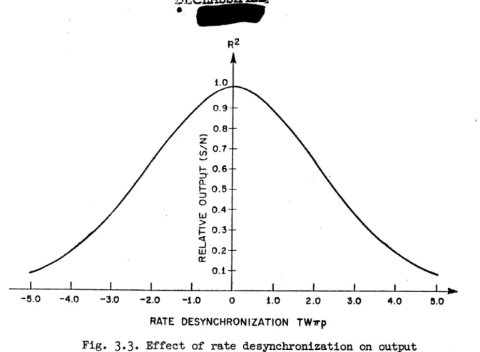
3.3

52

Effect of Rate Desynchronization on Output Signal-to-Noise

Ratio for Low-Pass or Matched Filter Detection of LowPass

Rectangular-Band Signals

3.-4

52

Relative Correlator Output Signal-to-Noise Ratio for

Sym-metrical Peak-Clipping

4.1

79

Block Diagram of Digital Signal Generator

4,2

80

Experimental Stored.Signal

System

4.3 84 1500.-sec Section of Output Noise-Like Signal Waveform

4.4

79 Block Diagram of Experimental System Using Stored Signal

Generator of

Figure

4L1

4L5 87 Stored-Signal Normalized Power Density Spectra for Three

Different Stagger-Tuning Configurations

4.6

87

/

Output Voltage Versus Time Desynchronization for

Experi-mental System

5.1

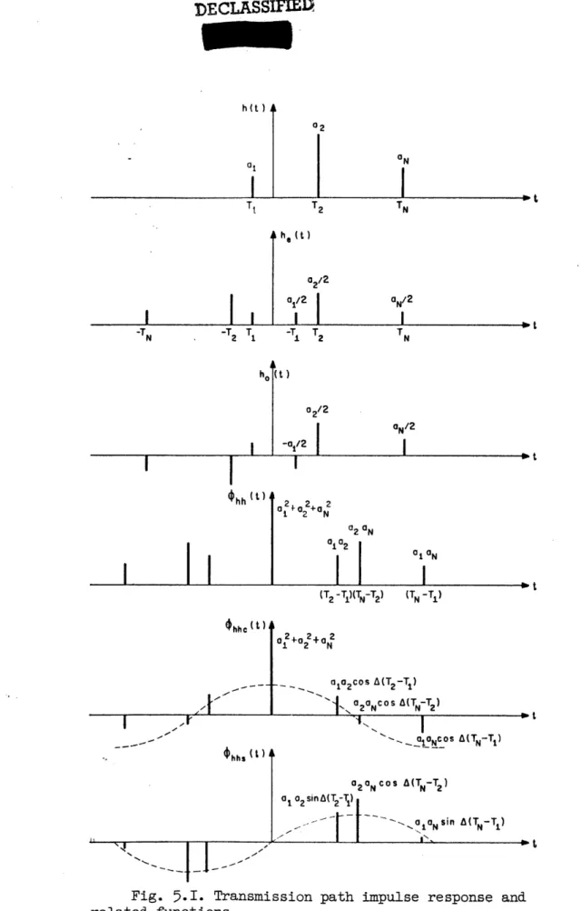
101

Transmission Path Impulse Response and Related Functions

5.2

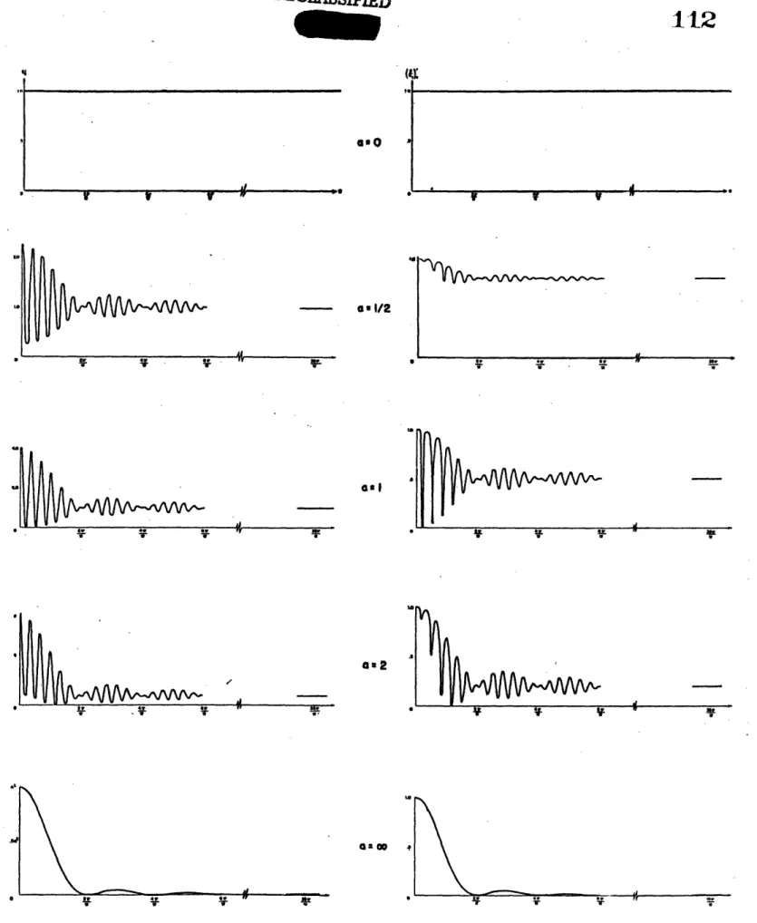
112

Signal Output Power and Signal-to-Self-Noise Ratio for

Stored-Signal System Using Band-Pass Continuous Detection

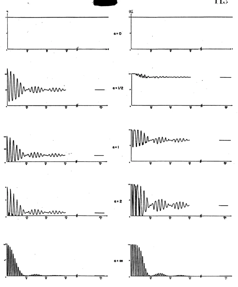
5.3

113

Signal Output Power and Signal-to-Self-Noise

Ratio for

Stored-Signal

System

using

Low-Pass

Continuous

Detection

5.4

114

Signal Output Power and Output Signal-toSelf-Noise

Ratio

for Transmitted Reference System

A.1

130

Driver Unit Schematic Diagram

A.2

131

Commtator Schematic Diagram

A.3

132

Resonator Unit Schematic Diagram

A.4

133

5-ac Oscillator Schematic Diagram

A.5

133

Sideband Generator Schematic Diagram

A.6

134

Channel Noise Source Schematic Diagram

A.7

134

Correlator

Unit Schematic Diagram

VTy .- p W '

I

DE(

CHAPTER I

CORREIATION DETECTION OF NOISE-LIKE SIGNALS

1.1 A Communication System Model

The basic purpose of any communication system is the transmission from one point to another of data in the form of certain messages chosen out of a set of possible messages. Such a system is the one schematized in Figure 1.1. The message emanating from the source and intended for the destination is assumed to be a sequence of independent symbols. Certain signals xi are used to represent the various symbols and these are sent by the transmitter to the receiver through an intervening medium

denoted as the channel. The action of the channel is such that it causes

the received signals yj to be in general different from the xi. In fact, since the channel acts on the xi in a random way, it is possible that a

given y may result from a particular xi one time and another the next.

Inasmuch as the sequence of symbols will not be known in advance at the receiver there will be for the receiver an ambiguity or uncertainty, even after receiving a yj as to which symbol was intended. Upon reception of a yj, the receiver must therefore deal with a situation described not by

a certainty as to which signal xi was sent, but only by the various prob-abilities that different signals xi were sent.

In some communication environmentsl these probabilities are actually available at the receiver, in principle, since it may be assumed to have knowledge of the a priori symbol probabilities p(xi) and of the channel

transition probabilities p(y/txi) (the probability that if xi is sent,

T' CLASSI FIE

W-~P

DECLASSIFIED

rJ_a) co ., 4-_o -,

I

H . PC4

DECLASSIFIED

o

a

.. Z - x

!

I

w w U w cr w

I

z

(/) 4 aC I a) C.) r,_a,4 r4 ra_{- I}

I

() raf U) a) o) -, ___ __-_ I l

n-DECLASSIFIED

yj is received). That these data are sufficient to determine the desired a posteriori probabilities p(xi/yj) can be seen by writing

P(Y/xi)P(xi)

P(xi/Yj)P(Yj),

(1.1)

from which

p(x)p(y

x.)

p(xi/y_j) = p(xi)P(Y-Xi) (1.2)

p(yj)

In the communication systems of interest in the present study the destination requires as its input the original sequence of symbols with as few errors as possible. The complete function of the receiver is there-fore not fulfilled merely by determining the various probabilities p(xi/yj);

it must go one step further and make a decision in favor of one xi or another and pass on to the destination the symbol represented by this signal. Clearly,

if the frequency of errors is to be made as small as possible, the receiver should consistently select the most likely of the transmitted symbols, i.e., that i for which p(xi/yj) is the highest.

1.2 The Case of Additive White Gaussian Noise

The probability-computing operation of the receiver takes a particularly convenient physical form for the case in which the effect of the channel is to add white gaussian noise to the transmitted signals. This type of inter-ference is defined by saying that it is a stationary random function of time

having a power density spectrum flat over any frequency range in which signal components are present and that its multiple-order probability distributions

are all multivariate gaussian. The assumption that the channel is characterized

DECLASSFTEn

pir ·*

4.

ED

only by additive white gaussian noise can often only be regarded as a first approximation to actual conditions, but in a great many cases it is a completely adequate model.

If the power density of this noise is N (watts-per-cycleper-second) it can be shown that the a posteriori symbol probability p(xi/yj) after reception of a given waveform y(t) is

Kp(x )e 1 N 0 To

,

(1.3) P(y)

where T is the signal duration, K is a constant, and x (t) is the explicit

form of the i-th transmitted signal. This expression defines the following operations at the receiver: Upon reception of a y(t), the mean-square-difference between received signal and a locally-available copy of each xi(t) is computed. If the x are equally likely (as we shall assume them), the decision is made in favor of the i for which this quantity is the smallest,

(otherwise an appropriate weighting of these differences with the logarithm of the p(xi) is seen to be necessary). It is seen that the channel

conver-sion probabilities -- p(y /xi) in Section 1 but actually densities, say w(y/xi) here -- need not appear as explicitly stored data but may appear implicitly as the reference copies of signals xi(t) and the mean-square difference operation.

A receiver performing these operations is schematized in Figure 1.2.

By rewriting the mean-square difference expression, we have

T T 0 0 T y (t)dt 2 0 rWCT,Aq-ST1S11 ... E i LI I

xi (t) -y (t) dt

xi(t)y(t)dt

,

(4)

x

;a (t) dt

DECLASSIF=E

where the first two terms are recognized as the energies of xi(t) and y(t) and the last as -2 times the crosscorrelation between xi(t) and y(t). This is the familiar crosscorrelation function x y(¶) evaluated at the origin, where

X( ' x(t)y(t +r)dt (1.5)

0

Therefore, if the x(t) all have equal energy, the minimum mean square

difference criterion for decision can be replaced by that of maximum cross-correlation. In practice this is somewhat more convenient since the mean-square difference operation requires that the reference copies of the xi(t) all have the same amplitude as those that would be received in the absence of channel noise, while this amplitude requirement is not present with crosscorrelation detection. All that is required is that the reference waveforms have the proper amplitude relative to each other.

1.3 Crosscorrelation Detection

The use of crosscorrelation techniques for the detection of signals in noise has received quite some attention in recent years, and several practical methods have been evolved for implementing this operation. The types most directly connected with the present study are depicted in Fig-ure 1.3 with appropriate nomenclatFig-ure, and will be described here and analyzed more thoroughly in Chapter II.

It should be noted that the output of these detectors corresponding

to each

xi(t)

is not

a waveform,

but a number.

These numbers are compared

in making the decision.

DECLASSIFEIf

_ x

L

U) 0: a 2

0:

.p $. 4 L 2 ( a ro .0u K C

DECLASSIFIED

ao +) Cd c I 0o l a C) u4 0Cd .0 +H UQ)a a, CH C II

t

+ n N 1-1

ar

I I i -I '

DECLASSIFIED

In low-pass correlation detection the signals x(t) and y(t) are multiplied and passed through an integrating circuit. (For convenience the representation x_i will now be written simply x since attention will

center on a typical correlator-and-signal combination.) If the action of this circuit is to perform exactly the integration of the product from t=O to t=T (as would be the case for the rectangular filter impulse re-sponse given in the figure), the output sampled at T is

T

fo(T) = x(t)y(t)dt (1.6)

the desired crosscorrelation. We will refer to the rectangular type of integrator characteristic as ideal. If the impulse response of the inte-grator does not have this rectangular form but is instead some arbitrary i(t), the process is spoken of as non-ideal integration and the output function of time is given by

t

fO(t)= S x(t)y(r)i(t-r)d¶ . (1.7)

The operation of matched filter detection involves a linear system whose impulse response r(t) is (apart from a constant time shift) the time

reverse of x(t), say

r(t) = x(T-t) . (1.8)

The output function of time will be

fo(t) W y(T)r(t-)d-- y(T)x(T-t+)dT, (1.9).

which is the crosscorrelation function

%xy

(of Equation 1.5) in real time with origin at time T. If x(t) is defined as nonzero only in the time

DECLASSIFIED

7

interval (0, T), the output sampled at time T is seen to be mathematically

identical with that given in Equation 1.6 for low-pass detection. In effecting band-pass correlation detection the incoming y(t) is multiplied not by x(t) but by a function x' (t) which is different from x(t) only in that all its frequency components are displaced by a constant frequency A from those of x(t). That is, if we express x(t) for example as

x(t)

=

e(t)cos(pt

+

0(t)

) ,

(1.10)

thus describing x(t) by the two time functions e(t) and

0(t)

and the fre-quency parameter p, then the last has a new value p- in

x'(t) = e(t)cos( (p-A)t + (t) ) . (1.11)

The product function is passed through a band-pass filter which is termed ideal if its impulse response has a rectangular envelope as depicted in Figure 1.3 and non-ideal otherwise. The envelope detector registers the envelope of the filtered difference frequency tone appearing in the output fo(t) due to interaction of x(t) and x'(t). Writing

y(t) = d(t)cos(pt + (t) ) , (1.12)

the output at time T from an ideal filter (of impulse response cos At in the range (O, T) and zero elsewhere) is

T

fo(T ) = I cos At e(t)d(t)cos( (Fp-)t +

(t)

)cos(pt+e(t))dt

O (1.13) which is

DEtCLASSIFIE

mNt T y A .I r W4'

F-~

~DECLASS1IE1

9

T T

E1 e(t)d(t)cos(pt + 0(t) )cos(pt + (t) )dt 1 x(t)y(t)dt

2 2

0

o

(1.14)

for the usual condition p )) A )) 1/T. The function of the envelope detector and sampler in operating on fo(t) is discussed in more detail in ChapterIIo

The use of the correlation function in studying random time functions first gained real prominence in the works of Wiener on the power density

spectra of such functions2 (1930) and on the filtration of random signals

by linear systems3 (1942). (It appears now that part of the former theory

was employed by Michelson4 on a heuristic basis as early as 1891.)

The possibilities of auto- and cross-correlation techniques for the detection of signals in noise was recognized by Lee and others5 in their

investigations of the practical ramifications of Wiener's theories. They used still a different type of correlation detector from those considered

above, namely the sampling correlator, in which a number of readings are made by sampling the functions x(t) and y(t) simultaneously. Products of corresponding samples then are added to approximate the desired integral of the product. This type of correlator is generally inapplicable in practice to the detection problem defined here because of the greater equipment complexity required.

The low-pass type of correlation was first studied by Fano6 and

Davenport7 using a point of view different from that defined above for

this type of correlator. It will be noted that in the previous discus-sion, the function xi(t) was considered to be the same waveform every time the symbol i is sent. The situation studied by Fano and Davenport

nECLASSIFrE

1

I I I I i

' . '}DECLASSs1tF

I

is that in which the observations are made not on the same explicitly defined signal function (of specified duration T), but on different portions of an indefinitely long function specified only on a statis-tical basis. This type of operation, which is sometimes very convenient in practical communication systems, will be termed continuous operation throughout the remainder of this paper. The term fixed operation will be used to describe the situation in which xi(t) is the same waveform segment each time the symbol i is sent.

The use of low-pass and band-pass type correlation detectors in the continuous sense for the detection of signals in noise was discussed by Fano.8 The notion of using a matched filter for signal detection is not

new, but its implementation into a system of the type outlined in Section 1.1 was first suggested, also by Fano, in 1952.9 (Incidentally, it should

be clear that "continuous" operation of the matched filter is not defined since the filter is constructed to have a fixed impulse response.)

1,4 NOMAC Systems

In the next chapter it will be found that a certain signal-to-noise ratio which is a central parameter in specifying the frequency of symbol errors, depends principally on the ratio of energy in each of the set of

signal waveforms to the noise density N so that the explicit form of the waveforms is to a great extent arbitrary. Because of this, it is possible to choose them so that their effectiveness against additive noise is sup-plemented by effectiveness in situations in which waveform structure is important. Such a situation is the military environment in which the sys-tems of the present paper are required to operate.

i.

.1

g

~~IEzL-SSIFE=

cf'

III

A military communication operation is characterized by a tactical

L h4~ ont

--I-

4U·

e-m;

lo__a~aIffi

ht

hawQ

--

L;LAU.LI.; UCIWWOLL t WdALO JLLV %li CiUU.LLC6.UULL ArLLfr:.LVt WllVJ5 'U.LuJyu Wi described in Section 1.1 as the transmission of a succession of symbols

(in private, it should be added) and a third party in the person of the

enemy. His purposes are to detect the communication and either disrupt it or recover the message for himself. The desirable characteristics then of the communication are, first, that its very existence be as dif-ficult to detect as possible, and second, that if intercept is inevitable,

the transmission be of such a type that jamming, analysis, or imitation be as difficult as possible. By choosing as the signalling waveforms ones which have an even distribution of the energy in time and frequency, the

first

of these requirements is served, since by

doing

so

the

possibility

that the ambient noise will conceal the transmission is enhanced. The

wide bandwidth feature is also desirable as protection against random

noise jamming, as will be seen in Section 2.6. If, in addition, the

wave-forms have to the outside observer a complex and "unpredictable" structure,

the system has a better chance against cryptanalysis and deception.

These requirements have suggested the use of signals in the form af

segments

of

random

noise, and communication systems using noise-like signals

detected by crosscorrelation have been termed NOMAC systems (for NOise

Modu-lation And CorreModu-lation). In the present discussion we will call noise-like any signals which fit the above requirements of deliberate complexity and even energy distribution in time and frequency, whether or not they actually

derived from such a source as thermal or shot noise, Physically, NOMAC sys-tems may be divided into several clear-cut categories, the division being according to the method by which reference copies of the x(t) are supplied.

I

I

DECiASSIIE

ZD

In the transmitted reference system the reference signals are all sent to the receiver concurrently with the message transmission over a separate "auxiliary channel" (as contrasted with the "intelligence channel" bearing the message). In the stored reference system the signals are

actually stored separately at transmitter and receiver as originally assumed. There is a subdivision into two types of stored-reference sys-tem, the stored-signal type in which the waveforms are stored as functions of time and read out of storage in synchronism with the incoming signal, and the matched filter type in which they are stored as the time-reversed impulse responses of a set of linear systems. Detection in the last type is by definition matched filter detection, whereas the stored signal type may use either low-pass or band-pass detection. It is customary to employ band-pass detection for the transmitted reference type since the intelli-gence and auxiliary channels must usually be separated in frequency.

The idea of using noise-like signals in a correlation type

communica-tion system seems to have originated in "Project Hartwell,lO" a study

project conducted at M.I.T. in 1950, at which time the transmitted

refer-ence type was suggested by Wiesner and the stored referrefer-ence type by DeRosa and Adams. One of the recommendations of this study project was that the

possibilities

of such systems be looked into.

Subsequent work on the

sub-ject has centered principally in Lincoln Laboratory, M.I.T. A detailed

exploration of much of the underlying theory, particularly the subject of

error probability,

has been made by Basore.l

A number of versions of the

transmitted reference system have been built and used

in

actual

communica-12

tion circuits,

and some exploratory work has been done on physical matched

filters 13

DECLA SSI

1.5 The Storage Problem

That attention in system development would center first on the trans-mitted reference system is only natural, since problems of signal storage

and synchronization

are

circumvented

by this type of operation.

The

trans-mitter signals may be currently chosen segments of the noise output of a

gas tube, for example.

However, this equipment convenience is bought at the expense not only

of error probability (since much of the transmitter power is used to send

the reference signals, and since the receiver must perform its correlation and decision operations using faulty, noisy reference signals), but also

at the expense of security. Since the signal waveforms are no longer known

only to transmitter and receiver, but are available to anyone having access to the channel, the hoped-for advantages against intercept, analysis, jamming, and deception are lost. Once the principle of operation of the system is

found out by the enemy, detection of the transmission and recovery of the message are simple, since the set of reference signals, the "key," is avail-able with no "cryptanalysis" necessary. Jamming and deception are easily effected by supplying the receiver with bogus intelligence and reference signals which it cannot differentiate from the legitimate ones.

These inadequacies of the present transmitted reference type system are so serious as to constitute a strong argument for the development of workable stored-reference systems, in spite of more difficult equipment realization problems. The stored-reference system is the point of emphasis of most of the remainder of this paper, the problem of actual equipment

realization being dealt with in Chapter V. This is preceded by a formulation

EEcLSSFE

ef

4

of the output signal-to-noise ratio parameter and an analysis of the effect upon it of various factors peculiar to the stored-reference sys-tem. The effect of multipath conditions on both types of NOMAC systems

is dealt with in Chapter V.

DEcLSSIE

:

CHAPTER II

OUTPUT SIGNAL-TO-NOISE RATIO

2.1 Significance and Definition of Output Signal-to-Noise Ratio It has been mentioned that the task of the communication systems considered here is to convey a sequence of symbols to the destination with as few errors as possible. Thus the significant quantity speci-fying the degree to which the system performs this task is the prob-ability of error.

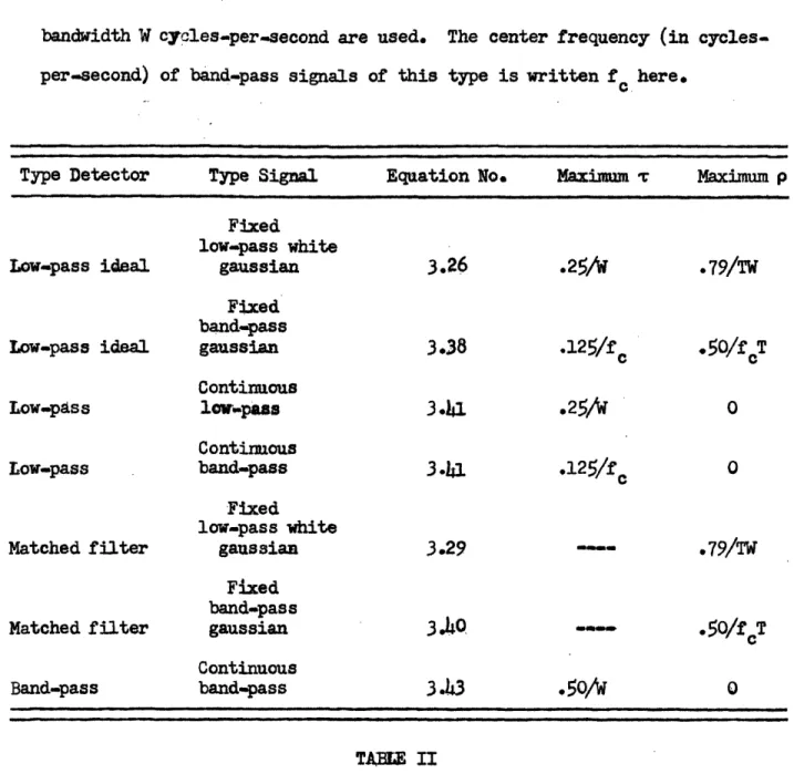
The results of previous studiesll of probability of error appli-cable to low-pass and matched filter detection can be stated in terms of 1) the number of equally-likely transmitter signals, 2) certain orthogonality relationships between these signals, and 3) a suitably defined output signal-to -noise power ratio from any one correlator. For fixed operation of the low-pass correlator, where x(t) is an explicitly determined time function, the output signal-to-noise ratio (S/N)o is defined in terms of the following hypothetical experiment: the crosscorrelation operation (Figure 1.3a) is performed once using each member of an infinite ensemble of additive noise waveforms of the specified statistical character. The output signal-to-noise ratio is defined as the ratio of mean output squared to output variance:

(S/N)= fo(T) /ff(To )

(2.1)

(Throughout this paper the bar will represent an ensemble average.) The

mean output is the ensemble average of the numerical readings which the

DECLASSIFIED

correlator registers at its output, and the variance is the ensemble average of the squared difference between each reading and the mean output. The definition of (S/N)o is applicable to the probability of error studies only when this difference is gaussianly distributed over the ensemble.

For continuous operation of the low-pass correlator, the function x(t) will be defined on a statistical basis only, and not as an explicit waveform. The output signal-to-noise ratio will then be the mean out-put voltage squared divided by the power in the outout-put voltage

fluctua-tions, this time the average being taken over the ensemble of infinitely

long noise and signal functions. Again the probability of error studies

require that the output fluctuations be gaussian.

For band-pass detection the pertinent studies of probability of error require that the signal-to-noise ratio be treated somewhat dif-ferently. Reference to Figure 1.3c shows that the numerical quantity

delivered from the detector is not a reading of the filtered product waveform, but a reading of the envelope of this waveform. The

prob-ability

of

error

is

specified

in terms of quantities

identical

to the

three enumerated above for low-pass and matched filter detection, except that the last of these, the signal-to-noise ratio is that at the envelope detector input. It is defined for continuous signals as the ratio of the

square of the average amplitude of the filtered difference frequency tone,

divided by the power in the fluctuation component of the output. This fluctuation component is presumed to have the character of filtered random noise. The use of a band-pass correlation detector under fixed conditions will not be discussed in the present paper.

Ls.

DECLASSIFED

rEC L SSFI

I(

In the remaining sections of this chapter the output signal-to-noise ratio will be computed for conditions somewhat more general than

those implicit in the original communication system model in which arbi-trary signal and white gaussian noise were assumed. Figure 2.1 depicts

the modifications to the block diagrams of Figure 1.3. The additive gaussian channel noise will be allowed to have an arbitrary spectrum, and independent additive noises will be assumed present in both multi-plier inputs for the case of band-pass detection, thus treating the situ-ation encountered in the transmitted-reference system (which customarily employs band-pass detection for frequency separation of the intelligence and reference channels.) Further, in all three detector types, one channel will be assumed to have in cascade an arbitrary linear two-terminal pair system. The precise character of this linear system will remain unspeci-fied for the present analysis. In later chapters its presence in the

signal-to-noise ratio expressions will be exploited in determining the

influence

of

certain factors,

such as multipath, on system

performance.

2.2 Low-Pass Fixed Detection

The noise n(t) indicated in Figure 2.1a is assumed to be a stationary and ergodic random function having a zero mean and power density spectrum N(W). The function u(t) is given by

T

u(t)

=

x)(z)h(t-)dr

.

(2.2)

0

Assuming the integrator characteristic ideal,

DECLASSIFIP

1.f.I x(t) C x(~t) lt) fo

xt)

,

1

¢tt )

, s

I

fo(t)

n(t) (b)

Fig.2.1. Correlation detectors of Fig.l.3 modified for (S/N)o

cal-f,(t) culation.

(a) low-pass type

(b) matched filter type (c) band-pass type.

(b)

(C) Fig.2.2. Spectra involved in

low-pass continuous (S/N)o

computa-tion.

(a) power spectrum of x(t) (b) power spectrum of u(t) (c) power spectrum of n(t) (d) X x N multiplier input term id) X x N multiplier input term

(f) integrating filter characteris-tic I(w)12. (d) (e) (O) POWER X U N XxU Id ... I.. Xx N

iia

3(t) a M~t P P ,- 0 r(t)

Fig.2.3. Vector diagrams repre-senting output signal and noise for band-pass continuous detection.

0ECLASSIrPInI

x(t) x'(t) n2(t) (c) ) U a) C , a (a) 0 (b) O

DEC'LASSIFIE

T f(T) = 0 pS·p l x(t u(t) + n(t)] dt so that T T fo(T) = [x(t)u(t) + x(t)n(t)]dt

5

0 0

since n(t)=O. If the Fourier transform of x(t) is

tie., W

x(t)

e'tdt ,

and similarly for U(co) the transform of u(t), then by the Parseval theorem,

fo(T) =1 (co)u(co) do (2.6)

u(c) = S()H() ,

fo(T) =

I()I

4H(co) do .

0

(2.7)

(2.8)

The energy density spectrum of the signal X(w) is defined as

X(c) =I (O) 0

(2.9)

Substituting this in the last expression and recognizing that it is even, whereas the imaginary part of H(c), written Im[H(o)], is odd we have

(2.3) (2.5) But so that I s-F t I

x(t)u(t)dt

(2.4)

DE

CLASSFI

:

f (T) =

The denominator of equation 2.1 is

2 T T

a

2

_{(f(T) ) =}

_f(T)-

_{fo(T) =}

0 0 x(t)x()n(tn(tn) dtd .

(2.10)

(2.11)

Since n(t) is assumed stationary, the ensemble average n(t)n(t) can be replaced by n(t')n(t' + T - t) where t' is any value of time while t

and are those in the expression to be evaluated. But because of the assumed ergodic character, this ensemble average may be replaced by the time average

8/2

lim

1

(2.12)

which is the autocorrelation function 0

n(t-t) of the random function n(t). By the Wiener-Khintchine theorem2 on such functions this is the inverse

Fourier transform of N(o),the power density spectrum of n(t). So the denominator becomes

21

T T o O

x(t)x(T)e'J(tr)dtd-

(2.13)

which is 1 2n S

(2.l4)

so that the output signal-to-noise ratio is

I

i

iI I

n(tt )n(t + ·e - tdt'I

UPCIASSIME17

X (o) Pe [ (.

d.

Fr~

mrcu~nerSStFIL

l [ X X(c)e [ H (o)] do

(2.15)

N

0

S

X(c)iN()do

For the case of H(o) identically unity and N(o)=No /2 (that is, No

for a single-sided frequency scale) in the region of nonzero X(a) we have

| 2 5 X()d 2 x signal energy (2.16)

o N

as was mentioned in Section 1.4.

I~~.s*_.

Z oJ Matcne. '±lter

Detection

The mathematical expression for fo(T), the quantity registered at the output of a matched filter detector, Equation 1.6, was found to be identical with that for fo(T) from the low-pass correlator for fixed operation using an ideal integrator. Therefore the above results, Equa-tions 2.15 and 2.16, apply to the matched filter as well.

2.4 Continuous Operation of. the Low-Pass Detector

To compute (S/N)0 in this case we proceed as follows: an ensemble

of stationary gaussian noise and signal functions all seconds long is

considered, where >> T. Each is expanded in a Fourier series and the

spectrum at the multiplier output is computed for a representative

ensemble

member in terms of the unspecified Fourier coefficients. The ensemble average power spectrum at the multiplier output is then gotten from this

L

DECLASSIED

VI-".- ~ ~ ~ ~ ~ ~ ~ ~ ~ c

I

"-I

based on known statistical properties of these coefficients. Then is allowed to grow without limit whereupon certain summations become inte-grals involving power density spectra. The power spectrum of the filter output is the input power .spectrum multiplied by the squared-magnitude of the filter frequency response. The signal-to-noise ratio is the ratio of the square of the d.c. component in the filter output to the remainder of the power, representing fluctuation.

For each member of the ensemble of signal and noise functions we have

the following Fourier expansions

i=l

n(t): =

ioos(X}t

·

+

yi)

(2.17)

i=l

u(t)

hcos

(Coit

+

i

+

7i)

i=l

where c_i represents the lower edge of a band of width W

cycles-per-second placed to include all signal and noise components, and hi and

7i

are IH(Owi) and arc H((i)] , respectively. It is known1 5 that when

x(t) is a stationary gaussian random process having power density spectrum X(c) (in considering fixed operation this symbol was used to represent an energy density) each i has a Rayleigh distribution over the ensemble with

i2 2 i 2 =2 i A (2.18)

· ~rCLssrsmD

D

LCLASSIFM2

and

and 4 2( 7) = 8 Xi 2(&A) (2.19)

where X is defined by . Xi = X(i). The phase angle i has a prob-ability distribution which is flat from - to +r. Similar statements hold for n(t) in relation to Z/i, i' and the power density spectrum

At the multiplier output there will be two distinct contributions

from the product x(t)[u(t) + n(t)l which we will denote as the (X x U)

and (X x N) contributions, respectively, using the subscripts I and II. Figure 2.2 depicts the line spectrum of the power of one ensemble member of x(t), u(t), and n(t) and shows how the operation of the multiplier produces the (X x U) and (X x N) components. (There are also components

about the double frequency which will be

ignored

since

they

lie outside

the filter passband.) The large d.c. output signal resulting from the

coherence between x(t) and u(t) will be noted in the (X x U) term of

Figure 2.2d.

For the wideband signals

of interest,

the

signal

band-width W will be large compared to that of the integrating filter.

This

is depicted in Figure 2.2f.

When the signals x(t) and u(t) are multiplied, the voltage at w =O is

VI(0) _ hicosXi (2.20)

2

i=l

and the power is

PI(C)=

V(O)=

Z

E

i4hiscos

z

1 Eh

.hicos

77

i

?h1cos

X

i(21)

(2.21)

E)CLASSFTED

;ff AW 1

DECLSS

Taking the ensemble average of this and then going to the limit as

-4

,

we have

lim

P()

lim

. e -- )P. M I --V. 2f X x (c) IHJ(c) Cos (co)t +

0 0

X(o) IH(o)I

(2.22)

Similarly the (X x N) term at zero frequency is

VII(O)'

2 :

Iicos(i

i

)

from which

II

4

i

I1i)

cos(ii)

PrhI

205%i(t)+O7

/I>Iiiti'

VZAcos

(,,ys)

(2.24)

and

lim g

()

=

lm

a

-*D. I(O) *

₂

₀

_J

0 N(c)X (ox) dt,

since i and Yi are independent

and

uniformly distributed from

-wr

to .

In the case of terms at output frequencies different from zero,

o)=2r/, n=l, 2, ... IW, we have for the (X x U) term

2

i 1 i+nhinc

+

i+

(2.26)

+

Z

$i+n

ihcos(

t

+ 0i

+

2 1

1

DCLASSIFED

Cos 77 () ]

(2.23)

(2.25)

I I V (,Tn

+ 'q i+1 - Ai)

-

Ain

if ) }

1DECLSSIMFID

=1

2os

nt

2 e

+ sin

2 i

Z

i inhin

)+lLflIf

(i+n' i+n- in i in c (i 77 i i+n)

i

·. . . sin(.

..

o )

+

.

. . sin(. . . .)(2.27)

Since the integrating filter bandwidth is much smaller than W, we are really interested only in the multiplier output spectral lines for which n ((Oi. If H() is a reasonably continuous function, we have, for small

n, that hk O+n and X ke

77

k+n' The second term above is thus negligible.

for sufficiently large Q, and

lim

2

2wn lim 4t

-- O Pi

=

-

-

X(o)X(o+

T ) IH(o+

2'n)

2

8

8~~~~i

cos 2 '7 ()do. (2.29) Go The (X x N) term is

(2yn)=

VII

-1

2vnt

2 $

+ 1 sin 2int

2 e

Vi

c

_os

n t-

₊

_in-

_i

)+

_i

i+nco

° s

(

+i

-

in)

0 +n

i+n /iicos (i+n

i

Z . . . sin(.

.

.)

+

. . sin(.

.

.) (2.30)

i

COL

AS

SmrED,

(2 rn =1

PI

12nh

[n+tjn

ncs(

_O

_2.8

la1-+

2

i

DECtASSiFIE.

from which

limp (2n)

= 1 limr

-*c

II

) 2

(-G

l T

a

2f) m 2r

N(.)X(

(+ -Tdco

d

-In 8 o

\

N(o+ 2 n) X(o) d] 0 (2.31)

Those terms that will pass through the integrating filter are for n < W, so with reasonably continuous spectra we may write

(2.32) 2Tr= O3 O n=O, 1, .., and li p (2vm)= li L T &--+ I ¢ O--0S

X (co) H(co)l 2 cos2

7

(o)do .

raio _(2.33)

For the second term Of limn,

-+d - PI(O) predominates, representing the

signal output. If we now form the ratio (S/N)o as the quotient of this term divided by all others, we have

[

0

·

x(coH(c)

l

7

(c)d

2

X(o)IH(w)I 2 cos2 V (o)d +

12

5

X(o)N( c)do

1 (2.34)

Wf.

Here use has been made of the definition for W _f the effective noise band-width1 6 of the filter

2

Tif= II()1 2d/Ima ()l 2 (2.35)

DECLASSIFIED

F 0s, 0 I __ __ _ ___

lim

2Trn

lim

6 WPII(-)= E --O 8

DECLASSIFTED

which in this case is

1im

r

n.

+

2I

2

2

2T

(2.36)

passband

z

I(O)

except zero

in which

I(X)=

5

i(t)e'jctdt

(2.37)

If H(co) is defined on the basis of a double-sided frequency scale, (S/N)0 can be written in a form more easily compared with equation 2.1.

(-) _N 2 (2.38)

Wf

2.5 Continuous Operation of the Band-Pass Detector

The analysis for band-pass continuous operation (Figure 2.1c)

pro-ceeds in a fashion almost identical with the preceding work for

the

low-pass case except that here the spectra of x(t) and u(t) are shifted apart

by A, which we will assume larger than the signal bandwidth. Therefore we seek as (S/N)0 the ratio of the squared amplitude of the

difference-frequency sinusoid passed by the filter to the remaining power, represent-ing fluctuations.

Independent additive gaussian noises having power density spectra

N1_{( )} and N₂(c) are assumed added to the upper and lower correlator in-puts of Figure 2.1c, respectively, so as to include the condition of operation of the transmitted reference type of system.

DEC

LASS

IE

i. ()

., ) HX

il~ d

DECLASSIFIED

The Fourier expansions which will be dealt with are now

u(t) = - ihiCos(coit + i+ X i)

1

(2.39)

n2(t) i cos [( A)t + 6i]

Again we will compute the power in the various lines at the multiplier

output, which in this case will be examined in the neighborhood of

the

difference frequency A. There are four sets of lines to be considered,

(X' x U), (X' x N1), (U x N2), and (N1 x N2) for which the subscripts I,

II, III, and IV will be used, respectively.

When x' (t) and u(t) are multiplied, the voltage at the difference frequency is

v(A)

=

2

CZi2h.

cos(At

+

i)

(2.40o)

I 2 i ' 1

and the power is the time average of V

2

(A) which is

P

( )

₁

_hi

_{+ 8[ho ihisin}

_cos

7

1I

7

(2.~ )

.4h

8

Cos

j2hjcos

8

hsin

i

E

3.

·

,ECLASSIED

The limit of the ensemble average of this expression as approaches infinity is lir P (A)

e

*----*o = lia 1 2 e-&

2

X 2_{(co) H(co) Zd}

+ :

()

H(cos

l

co(o)

a]2

+ 1

X

() H

s

(co)

dJa

0

.

The contribution at )=A of the (XI x N1) term is

V (A) 1 :

i Ji cos(At

i Y

2 i i

(2.43)

from which

8

i/cam

·

jj

a

+I.

1

i

sin()i-

Yi)]P

(2.44)

and

lim P

lin

2 e 02

o

Similarly we find the (U x N2) and (N1 x N2) terms at c=A to be

Um P (A), =

0 -* M III(

e

a and im P

()

=

im

ae-.#

4 TV I8 -co

12 t

I

1

21

2

e J

XI()IH(c)I N₂ (co - A)do

respectively.

DECLASSIFIED

(2.42)

I

(2.,45)

(2.46)

(2.47)

X (co N, (o) de N1 (c)N2(co " Q Ck

VV'.

f

rRT1TVT

t.

By repeating these four calculations to find the contributions the power at other frequencies we find at =A=2n/@ where n + 1, +

+

~W

that

li

p(2m

+

eX

lim 1 2=t

X( +

) H(

2

rn)

68 -- *

( + . 0

P

X(o)X(o

2

+

ni)

H(o

+

(2 .h) lim (Ttn 2P a) = lim 1 2n l*G iT a - 2

\

X(co)N(o +

2n)d

(2.49)

IoJ

6

lim

Tn

+ = li 1 2n e- 2 8 So

X(o) H(co)

2

N

2

(,a+

2n)

d

(2.50) and li (2 n A) lim 1 27 &---V W IV

e

a _ 2 a

N

l

()N

2

(o

- A

+

2n)d

0

(2.51)

Again with the integrating filter

bandwidth much less than W, and for

reasonably well-behaved signal and noise spectra, only those fluctuations

components close to oi=A will pass through the filter. The desired output

signal-to-noise ratio is the ratio of twice the power in the difference frequency tone (the squared amplitude is twice the power) divided by the fluctuation power, and so collecting terms we have

-OECLASSIFWIE

to 2, ...

2

o 2

0 Xi(c)Re[H(co)] d3 + [ X(@) Im[H() da] 2

0 0

(2.52)

where here the effective bandwidth of the integrating filter is written

2~r

=

I

> 2I() 2Tr (2.53)

-f

passband

II()l

2

and where, as before, the channel filter characteristic H(o), is rephrased in terms of a double-sided spectral representation. The noise spectra may be regarded as either all single- or all double-sided without the

expression being altered, since it is a ratio of powers. However, it must be carefully noted that the range of the integrals must include only the half-range 0 to infinity, because of the second numerator term.

2.6 Interpretation and Remarks

If one compares the expression for (S/N)o for fixed operation (equa-tion 2.15) with those for continuous opera(equa-tion (equa(equa-tions 2.38 and 2.52), one is struck by the presence of the extra denominator term in the latter, a term which does not involve the channel noise. This part of the fluctu-ation power is called the self-noise. In continuous type operfluctu-ation since measurements of the energy, equation 16 , are made on different portions

of the same signal function, instead of the same portion as with fixed

E)

f' .j

operation, there is this fluctuation in the energy which is seen to

de-crease

as the

observation

interval

widens.

7

_'

1 7

_{In the low-pass detection}

case, this self-noise can be assumed to have the required gaussian

dis-tribution

by virtue of the small bandwidth of the

filter

compared

to

the

bandwidth of the self-noise spectrum before filtering.8

When the self-noise term becomes the predominant denominator term in the band-pass expression (equation 2.52) for (S/N)o, it must be used

with some caution in determining the probability of error.

This is

be-I. -

Ol

n..44-4

_hU- l.

-ho -AQU

b

a

f

--

tf

I;,LL~;

W J)C;~bl

4itL:

LLQL pJJ.UdULL. Jl UJ. B.LXIJ.L' OO-I. LVOL 4U LJ deau VL bLW

assumption that the output noise power is narrow band gaussian noise re-presentable as1 9

f(t) = (t)cos At + p(t)sin At (2.54)

where a(t) and p(t) are independent and gaussianly distributed with zero

mean and variance equal to that of f(t).

The last three denominator terms

1mnr

', ,vMr,r+.MrA

+i' h,'r, +

a

a;

hmral,,a Fv,

l+h

'h.i

(:11

II

hanMtT-;rth

fi

p

the integrating filter and because there is no coherent structure in the filter input spectra giving these three terms. However, if one sets

(,,A=

t

rn'(.ant

Anr.

.

a:-ins th

lPf'nn';A.

era'i.

m in t.he

derivatinn

of (S/N)o, it is found to be symmetrical about c=A so that even though

the self-noise output may also be considered approximately gaussian due to narrow filter bandwidth, it cannot be expressed in the above way, but

instead as

f(t) = (t) cos At (2.55)

(which is seen to be non-stationary) the difference being in the absence of any phase modulation.

Lh.

nCLASSIED:

:

41.

i. 11.,

DECLASSIM

D,

It turns out that when H(o)= a constant, the (S/N) expression (2.52) is still correct for the high output signal-to-noise ratios used in practice if the self-noise term is multiplied by two. This

can be shown as follows (Figure 2.3): The large horizontal vector of length P represents the signal sinusoid. The narrow band gaussian

noise of equation 2.54 is then represented by the resultant of the two small vectors having length (positive or negative) equal to a(t) and (t), Figure 2.3a. The envelope detector will register the length of the signal-plus-noise vector which is

(P + a) / cos 8

where

(=sin-l(P/Psa).

For sufficiently high signal-to-noise ratio, p <( P and the vector length is P + a(t). The variance of a(t) is the same as that of f(t).

In Figure 2.3b the case of equation 2.55 is depicted, and here the variance of y(t) can be shown to be twice that of f(t). Therefore in determining the effect on the envelope, the self-noise power must be multiplied by two when the complex self-noise spectrum is symmetrical about the difference frequency A.

When H(w) is not a constant, then it is not clear just what the behavior corresponding to Figure 2.3 will be, since the self-noise spectrum is neither even, nor are the parts on opposite sides of the carrier completely unrelated. It is conceivable that the orientation of the vector representing output self-noise power be more perpendicular on the average than parallel to the signal vector, thus reducing the probability of error. In the absence of more investigation of this

TCASSI

DECLASSRF]

I

problem, the safest thing to do is to compute probability of error on the pessimistic assumption that all the self-noise power is concentrated in the orientation of Figure 2.3b. Equation 2.52, modified by inserting

a factor of two in the first denominator term, still stands, but it must

be remembered that when self-noise is predominant and H(c) is not a

con-stant, the probability of error may actually be lower than computed.

Expressions 2.15, 2.38, and 2.52 are somewhat unwieldy in their general-ized form as they stand, and it is useful to rewrite them for certain partic ular situations of frequent occurrence.

First, if the noises and signal all have the same spectral shape, and if H(o)=constant, then the reciprocal of (S/N) is

K

~

(i)

(2.56)

o 2TW S i

X

for low-pass fixed operation or matched filter detection (equation 2.15). Here (N/S)i is the ratio of average noise power to average signal power

at the correlator input, T is the symbol duration as before, W is the

x

effective bandwidth of the signal energy density spectrum (co), and K is

a spectrum form factor

K

=d (2x57)

x

(c)

X(c)~

..

a few representative

values of which are given

in

Table I.

For low-pass

continuous operation (equation 2.38) ,we have

f

lN

K( +-( )

(258)

I~~~~~~()__w

i- -~~~~~

(

E

CrbCa

ASSrWT

.1 I :-C., I;

-i. ASS,. .',,,

where

W and

K are computed from the power density spectrum X(c). For

x

band-pass continuous. operation.

() 0 Wf

x

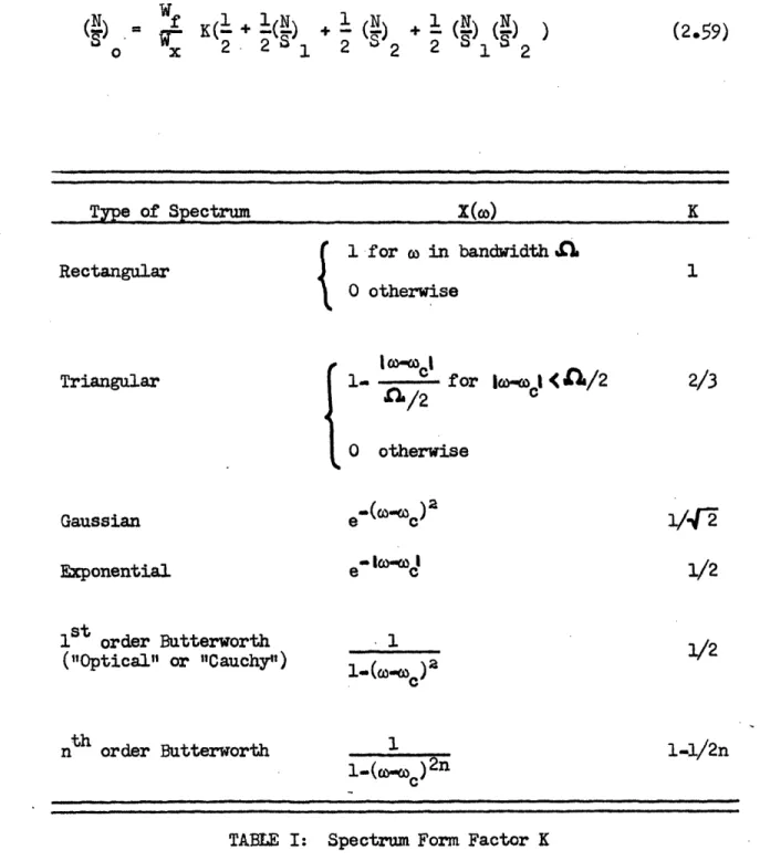
1 K(2 2 - 1 2 2 +2 2 (1 1 S 2 )2

(2.59)

Type of Spectrum

X(o)

K

1 -for

co

in bandwidth

n

Rectangular

1

0 otherwise

Triangular

1 .

C

for lC.%l <

SA/2

2/3

O otherwise

Gaussian

e'*((C)

1/42

Exponential e' IcO- 1/2 1S t order Butterworth 1 2

("Optical" or

"Cauchyt')

nt order Butterworth

11-1/2n

c ,

TABLE

I:

Spectrum Form Factor K

D)ECLASSID

r_-vr

D ZEC

C

-1.

"'

S

1SS3i.

where (N/S)1 and (N/S)2 are the noise-to-signal power ratios at the two

correlator inputs.

For the case of white channel noise, with H(c)=l, we have the result of equation 2.16 for fixed operation, and for low-pass continuous opera-tion,

W

N

()

=-f

(K

+

o

(2.60)

So w

_wx

2X

_2max

For band-pass continuous operation

W N w_ T _ N .\

(N) (+ _0 + + 20l2 + 02:. + ) (2.61)

S 0 W 2 2Xmax 2X 2 X

2

W

X max max max x

where N01 and N 2 are the spectral densities of noise at the two correlator

inputs, and Wt is the bandwidth of these white (rectangular spectrum) noises, WI being assumed large enough to include all of X(co). These expressions

ow

mo+h

-4

ho

I--

cmat-

+

c,+

4

mil

+r- +.hs

4--

n-rA in

nv.ro +

++

+

4

no-lla+

i'"

"

c

Ian

to-signal ratios are redefined in terms of power densities.

Equations (2.59) and (2.61) point up a fundamental disadvantage of the transmitted-reference system compared to the stored-reference system, namely the much lower output noise ratio for a given input signal-to-noise ratio. Specifically if the channel signal-to-signal-to-noise ratio is a quantity p somewhat less than unity, (S/N)o for the stored-reference system is p times 2 W KWf. However, for the transmitted-reference system with a small signal-to-noise ratio p in intelligence and auxiliary channels, (S/N)O is p2 times 2 W KWf.

tDE CLASSIF TED

E L~DECLASSNIED

Although in the analysis of fixed type operation, the character of the signal was arbitrary, it will be recalled that it was specified as a gaussian random function for the case of continuous operation. (Sections 2.4 and 2.5) A review of this analysis will disclose that except for the self-noise denominator terms, the results (equations 2.38 and 2.52) are still correct for non-gaussian signals. All that is re-quired is that, as in equation 2.18, a constant ratio exist between the second moment fi2 of the Fourier coefficient i and the power density spectrum X(X). (The behavior of the fourth moment 4 is seen to enter only in the self-noise term, and the phase «i not at all.) This condi-tion exists in general for well-behaved funccondi-tions of tLme, since if it is valid to expand in a Fourier series segment of the function seconds long, as 8- the average power contained in any one Fourier spectral line at i must become identical with the power in that part of the power density spectrum from i- 1/0 to i + T/g,which is asymptotically

X(

i

) 2 = X(

i)

.

(2.62)

It is of collateral interest to use the general expressions for (S/N)o in determining the effect of noise jamming on NOMAC system per-formance. Specifically, we might ask what spectral shape N(c) of jamming power will be most effective in reducing (S/N)o for a given jamming power. For the stored-reference system (equations 2.15 and 2.38 with H(Q)=l, and 2.52 with H(c)=l, N₂=0, and N1=N(c) ) this means maximizing

X (co) N(co)d (2.63)

DCEASSFI

DECLASSIFIED

while constraining

o

0

If X(o) has a maximum value Xmax at some frequency o1' the N(o) should be

an impulse (of value PN) at this frequency, whereupon

X()N(co)do = Pmax (2.65)

o

If instead N(o) is for example rectangular with width

)L

and therefore height P , then we must have

X (co)N(co)dw

*

N X ( (2.66)

since no values of X in

Cn)

are greater than Xmax. (The equality sign holds

if X=X everywhere in A .) The output signal-to-jamming ratio is (from

equation 2.52)

2W

A(.)= Wx-(S) (2.67)

J W J i

f

where (S/J)i and (S/J)o are the input and output signal-to-jamming power

ratios. Thus it is seen that no distribution of jamming power is more effective than an extremely narrow concentration of power in frequency, and this jamming frequency should be adjusted to coincide with the fre-quency of maximum signal power. The advantage of wide-band signals against jamming is now apparent since if the best the jammer can do

nDCLASSIIEl'

e8

") ;A